Development of a GPS Forest Signal Absorption Coefficient Index


1
Department of Geography and Environmental Engineering, United States Military Academy, West Point, NY 10996, USA
2
School of Forest Resources and Conservation, University of Florida, Gainesville, FL 32611, USA
*
Author to whom correspondence should be addressed.
Forests 2018, 9(5), 226; https://doi.org/10.3390/f9050226
Submission received: 14 March 2018
/
Revised: 19 April 2018
/
Accepted: 20 April 2018
/
Published: 25 April 2018
(This article belongs to the Special Issue Remote Sensing of Leaf Area Index (LAI) and Other Vegetation Parameters)
Abstract
:In this paper GPS (Global Positioning System)-based methods to measure L-band GPS Signal-to-Noise ratios (SNRs) through different forest canopy conditions are presented. Hemispherical sky-oriented photos (HSOPs) along with GPS receivers are used. Simultaneous GPS observations are collected with one receiver in the open and three inside a forest. Comparing the GPS SNRs observed in the forest to those observed in the open allows for a rapid determination of signal loss. This study includes data from 15 forests and includes two forests with inter-seasonal data. The Signal-to-Noise Ratio Atmospheric Model, Canopy Closure Predictive Model (CCPM), Signal-to-Noise Ratio Forest Index Model (SFIM), and Simplified Signal-to-Noise Ratio Forest Index Model (SSFIM) are presented, along with their corresponding adjusted R2 and Root Mean Square Error (RMSE). As predicted by the CCPM, signals are influenced greatly by the angle of the GPS from the horizon and canopy closure. The results support the use of the CCPM for individual forests but suggest that an initial calibration is needed for a location and time of year due to different absorption characteristics. The results of the SFIM and SSFIM provide an understanding of how different forests attenuate signals and insights into the factors that influence signal absorption.
1. Introduction
The Global Positioning System (GPS) constellation is primarily used for position, navigation, and timing purposes. However, the scientific community has used the signals transmitted from GPS satellite vehicles (SVs) for applications in many different research fields. Some GPS signal studies include GPS performance, wireless communication reliability, and the combination of GPS signal-to-noise ratios (SNRs) with light detection and ranging (LiDAR) data to measure signal loss in forests [1,2,3,4,5]. The L1 frequency of the GPS system broadcasts at 1575.42 MHz and is attenuated by vegetation. Developing a method to predict with confidence the degree to which GPS signals are affected by forest structure provides useful information on L-band scattering and absorption. This work is important to understanding GPS performance and to scientific studies that employ other microwave signals, such as satellite communications, air-to-ground communications, cellular phones, and synthetic aperture radar (SAR). It is also relevant to studies that explore forest growth modeling and use light interception predictions [6,7,8,9,10,11,12].
Both in previous studies and in conventional SAR remote sensing applications, forest vegetation is generally assumed to be uniformly-distributed stratified media [13]. This builds on Beer’s Law and suggests that the zenith angle of the microwave source is a key factor governing the scattering of radio waves in a particular forest stand. However, ecologists have long recognized that forest structure is far from uniform.
In the literature, there are many different techniques used to model signal loss through forest structure. For the research presented here, the most relevant model is the Canopy Closure Predictive Model (CCPM) described in [14]. The CCPM model consists of capturing two primary components: one based on the atmospheric attenuation, and the second based on attenuation by the forest canopy based on Beer’s Law. When considering Beer’s Law, if we consider the forest as a uniform slab of vegetation, the absorption of a signal exhibits a linear dependence between the signal propagation path length through the media, an absorption coefficient, and the concentration of medium yielding:
where is attenuation, is the path length, is the concentration of the media, and is an absorption coefficient [1]. The CCPM was developed for a managed pine forest and the Beer’s Law component consists of the product of the sine of the zenith angle and the canopy closure value. The CCPM makes the assumption that the concentration and absorption parameters of Beer’s Law can be combined into just the canopy closure (CC) of the forest, where CC is the percent of pixels classified as canopy in a window of interest inside a hemispherical sky-oriented photo (HSOP).
As such, there is a need to determine the concentration of the forest through the path of signal propagation [5]. Our hypothesis is that while zenith angle may be the dominant factor in attenuation, other independent parameters leading to variations in signal strength will be observable, and that the inclusion of HSOP-derived CC data at 1-degree zenith angles can precisely measure the degree to which GPS signals from individual SVs are affected by forest canopy.
The goal of this study is to estimate the values of L1-band GPS signals in multiple diverse forests using observations from GPS and CC values derived from HSOPs. The objectives are to (1) develop an atmospheric attenuation model for GPS SNR values, (2) develop an overall canopy closure predictive model (CCPM) independent of study site, and (3) create an adjustment index for each study site that can be applied to the CCPM in order to allow for refinement of predictions based on forest absorption characteristics.
2. Materials and Methods
2.1. Study Site
The data used in this study were collected in 15 different forests throughout the United States. Figure 1 depicts the location of each forest and Table 1 provides forest details, including the date of each data collection, the average and standard deviation of both the diameter at breast height (DBH) and tree height, and a brief description.
The vast majority of data were collected during the summer of 2015 (Table 1). Due to personnel availability constraints, weather conditions varied between each location. In each case, best efforts were made to collect data in the morning or during times with mostly-cloudy conditions to avoid sun glare on the images. During this data collection period, California had a lack of winter precipitation and was in drought conditions. In contrast, the gulf coast region had higher precipitation than usual.
2.2. GPS Signal Observations
To obtain a measurement of signal loss, GPS L1-band SNR observations were collected both in the open and inside each forest. Four Topcon Hiper Lite global navigation satellite system (GNSS) receivers were used, with three receivers set up inside each forest and one receiver positioned in an open area within 1 km of the others. Comparing SNR values observed from the GPS receiver in the open to those in the forest provides the signal attenuation observed at a specific site at a specific time. The three receivers that were set up inside each forest were positioned at random locations and recorded at least 60 min. of observations. The observations included multiple National Marine Electronic Association (NMEA) messages at a rate of 1 Hz. The recorded messages included: time, GPS SV SNR values, GPS SV zenith angle, and the azimuth of each SV with respect to the GPS receiver. We collected data from an average of 10 GPS SVs, resulting in 36,000 observations per GPS receiver, per data collection. As such, given 19 data collections, each with four GPS receivers, the data used in this research includes over 2.5 million GPS SV observations. It is important to note that for each GPS receiver setup, we calculated the mean SNR for each SV at 1-degree increments from the horizon and used these values in the modeling process.
A control experiment was conducted in January 2015, where all four GPS receivers were set up within 20 m of each other in the open. No statistical difference between each GPS receivers’ SNR observations was observed [15].
2.3. Hemispherical Sky-Oriented Photos and Image Processing
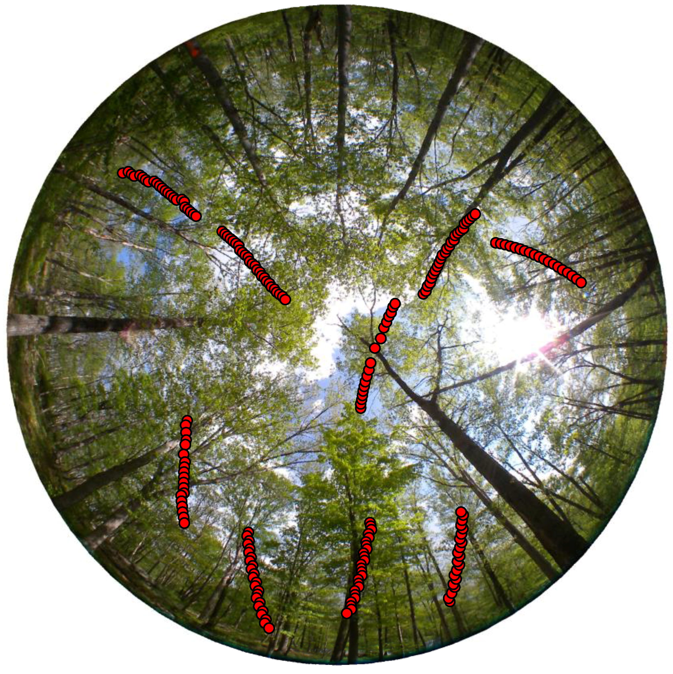
A single HSOP image was taken at each GPS receiver setup location in each forest with the camera directed straight up, and the top of the photo oriented north. The resulting photos are circular, with zenith in the center of the image and the horizon on the outer edge. An example is shown in Figure 2. The camera and lens combination used to collect these images consisted of an IPIX fisheye lens mounted on a Coolpix P6000 Nikon camera (Nikon Ltd., Tokyo, Japan).
Figure 3 shows the frequency distribution of the number of GPS SV observations recorded during the spring data collect at West Point, NY.
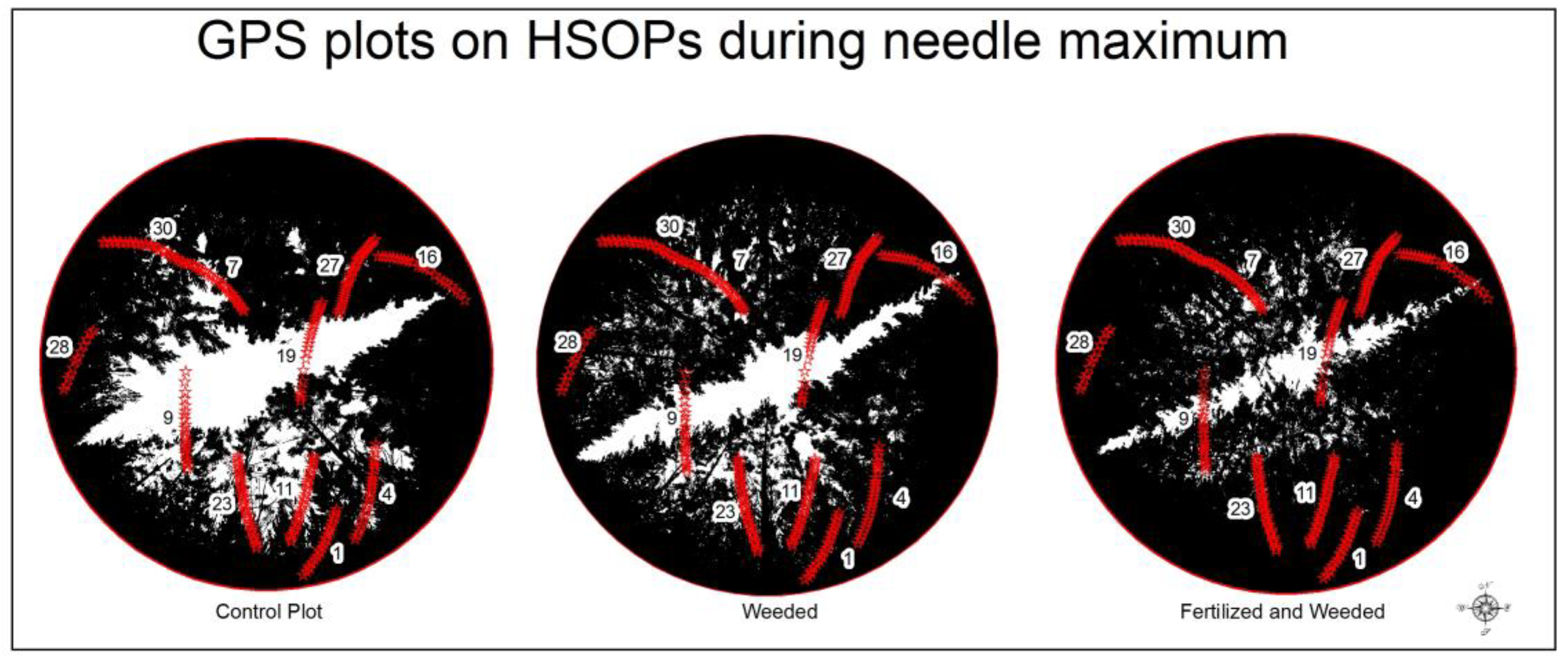
Image processing of the collected HSOP images was conducted using ArcGIS software (Environmental Systems Research Institute (ESRI), CA, USA). ArcGIS allows for the establishment of spatial reference, the delineation of each photo into one-degree rings associated with each angle from the horizon, and the ability to convert each image into a binary, black and white, image, where the sky is white and forest structure black. Tools within ArcGIS allow for the isolation of the blue channel of each HSOP for the creation of the binary image. This is beneficial because the blue channel is better suited to distinguish clouds and sun glare [16,17,18,19,20,21] than the red and green channels. When creating the binary image, the Natural Breaks function was used to determine appropriate threshold values. Additionally, each histogram and binary image was visually inspected for accuracy. During this process, each Red, Green and Blue (RGB)histogram and corresponding open-sky threshold values were examined to ensure there were no abnormalities. The resulting binary images were then compared to the original images to ensure proper classification. Figure 4 and Figure 5 are the resulting binary HSOPs from the Intensive Management Practice Assessment Center (IMPAC), a managed forest in Gainesville, Florida, during needle minimum and needle maximum. The three plots in each of these forests were unique in that the species and spacing of the trees were the same. The difference between the plots resulted in different fertilization processes resulting in different DBH and tree heights between the plots.
During image processing, the percentage of pixels classified as canopy at specific angles from the horizon inside each specific forest was calculated. These CC values serve as the concentration of forest media at specific angles inside the forest. Instrumental to our modeling process is the calculation of CC fractions for each angle from zenith. This was conducted using the zonal statistics tool within ArcGIS for each 1° ring, as shown in Figure 6. Using the zonal statistics tool, the corresponding CC value for each SV location was extracted for use in statistical modeling.
3. Results
The models presented below are the results of regression modeling. This process consisted of initial data exploration of many different variables other than those presented. During the analysis, we identified ways to linearize the relationships within each model. Four models are presented and include an atmospheric model, a model optimized using HSOPs, and two models using dummy variables for each forest to generate an absorption index associated with the different forests.
The first analysis conducted used all the open receiver GPS observations to create an overall GPS SNR atmospheric model. In this work, we built on the previous work where the natural log of the angle from the horizon () of the GPS SV was the key parameter in the modeling process [21]. The resulting overall GPS L-band SNR atmospheric model (SAM) has a Root Mean Square Error (RMSE) of 2.01 dB and an adjusted R2 of 0.81. The SAM equation applies to all observations where no vegetation is present over the GPS receiver. The SAM equation is:
When exploring how different forests influence GPS signal, we incorporated the use of the CCPM. The CCPM approach to model SNR incorporates GPS observations from all forest study sites. The CCPM uses two variables. The first variable is , as in the SAM equation, which linearizes the problem and is also vital in modeling the atmospheric component of the observed SNR. The other variable in the CCPM is the Beer’s Law component, the product of CC and the sine of the zenith angle. Table 2 shows the results of the CCPM for each individual forest, with the equations taking the following form:
where is the natural log of the angle of the SV above the horizon, is the zenith angle, and SNR units are in decibels.
The last model we developed incorporated all aspects of the CCPM and also included dummy variables associated with each different forest site. The resulting dummy variables simply provide a Y-intercept shift for the expected SNR value based on a particular forest. The resulting dummy variable coefficients for each specific forest provide absorption indexes that help establish an understanding of how each forest affects the reception of GPS signals. The resulting model is termed the SNR forest index model (SFIM). The SFIM had an RMSE of 3.24 dB and an adjusted R2 of 0.65, with the SFIM equation is as follows:
where I is the index value.
Inspection of the SFIM equation shows that the Beer’s Law component has a very small influence on the model. This result was unexpected initially. However, it agrees with the same points as discussed with respect to the overall CCPM model applied to multiple forest sites. Based on the lack of influence by the Beer’s Law component, it was removed from the model to generate the simplified SFIM or SSFIM. The resulting SSFIM equation is:
The SSFIM resulted in the same RMSE and adjusted R2 as the SFIM. Table 3 shows the results of the absorption index value (I) for each forest applied to the SFIM and the SSFIM.
4. Discussion
In the first portion of this study, we presented the SAM. The SAM methodology is simplistic and, as such, future work associated with atmospheric modeling has been considered. Factors such as humidity, barometric pressure, clouds versus open sky, and fog could all be potential components in atmospheric modeling. However, many of these factors change rapidly and would require a very substantial series of photos and measurements of the different variables over short periods of time, thus we used the approach outlined above to develop the SAM.
A primary objective of this research was to determine the parameters that influence signal attenuation. As such, during the modeling process, many other variables were considered to include the interaction of these variables. Parameters such as the leaf area index (LAI) (as calculated from gap light analyzer software), the density of the trees, average diameter at breast height, and average tree height (to name a few) were considered. However, the parameters that make up the CCPM and SSFIM proved the optimum method.
Many previous studies modeled forest structure. Larsen and Kershaw explained the evolution of different canopy structure models as the assumption of uniformity of foliage was removed [22]. Building on this work, Oker-Blom modeled forests with individual cylinder or parabolic crowns as trees with a uniformly distributed LAI density [23]. This work allowed for areas with no foliage and areas with overlap. The overlapping areas would cause a clumping effect. Other statistical models such as the Poisson, negative binomial, and Markov models predict the likelihood of a ray of light passing completely through forest canopy [24]. A great advantage of the models presented in this research is their simplicity. When comparing a single layer canopy to a triple layer canopy, for example, we simply obtain different CC values. In a triple layer dense canopy, there will be higher CC values compared to a single layer forest canopy.
The results shown in Table 2 suggest that for each individual forest, the CCPM performs well. However, when applying all the observations from each forest as a whole, the Beer’s Law component was not found to be statistically significant at 90% confidence. This goes against our initial hypothesis. However, based on the results for dummy variable modeling for seasons at West Point, it is not surprising. The West Point seasonal study found that applying dummy variables for the seasons helped adjust the overall model [21]. This adjustment likely had to do with the health of the canopy. For example, during the fall season the CC values derived from HSOPs included foliage that was dry. However, these leaves were counted the same as leaves during the spring or summer that were healthy. Applying the same logic for different forests, each study site has different conditions. Some sites had received recent record rainfall while other sites were in drought-like conditions. Additionally, when comparing many different species of forests there are numerous factors that could influence the absorption component associated with Beer’s Law. Most importantly, Beer’s Law has both a concentration and an absorption component and the CCPM attempts to capture both using just CC. Therefore, it is justifiable that individual forests, sharing many of the same attributes, are successfully modeled individually using the CCPM, but as a conglomerate, the model does not work as well. As a result, the use of the CCPM is effective but would require a calibration prior to implementing for a specific forest, meaning that when photos are taken in a forest to get the CC values, GPS SNR observations should also be collected. If a GPS calibration is not feasible, a user of this work may benefit from a different approach, such as the SSFIM.
When comparing the results of the SFIM to the SSFIM, we identified that the SSFIM provides an equation that removes the need for photography. With both models having the same RMSE and adjusted R2, ultimately, there is no need to go through the added complexity of taking photos. Rather, a user can reference Table 1 and Table 3 to identify a forest with similar attributes and gain an insight into how signals may be attenuated in a particular forest site. The challenge with this concept is identifying what the key similarities are between forests. Would species play the largest role, or would tree height and DBH have a larger influence? In a similar vein, there is a seasonal influence on attenuation, as shown in Table 3 at the West Point study site. As such, a larger index is needed with more forest types. Further research is also needed to determine the variability of absorption within a single forest based on rainfall, foliage conditions, and other factors to ensure a good prediction of signal attenuation. All of these are just some of the questions that could be addressed in future work.
5. Conclusions
In this study, four different GPS SNR models were presented: one model predicts GPS SNR in the open and three models provide methods to predict GPS SNR in forest conditions. Previous work shows how applying predicted SNR values can easily be applied to determine estimated attenuation. While we expected all models to perform well, we were initially surprised that the CCPM did not perform well when modeling all forests together. However, when considering that the CCPM uses only CC to describe the Beer’s Law component of signal loss, these results reflect that absorption variation is significant between different tree species and environmental conditions. The SSFIM accounts for this variation nicely according to its associated results.
This work specifically investigates GPS signal attenuation in different forest conditions. However, gaining a better understanding of techniques to model GPS signal attenuation will lead us to understand how other signals belonging to other technologies may be influenced. Technologies dependent on different cell phone frequencies, satellite communications, Bluetooth, and AM or FM radio transmissions are just a few of the different signals that could benefit from the presented predictive models. This work could also benefit forest growth research that uses light interception predictions.
When this research began, it was our desire to build on the knowledge of how GPS signals are attenuated in different forest environments. There was no desire or requirement to limit our modeling efforts to any specific technologies, only the desire to try as many different techniques available to us and identify the optimal modeling approach. The use of HSOPs in the modeling process proved fruitful from the beginning of our work. The historic use of HSOPs to estimate LAI led us to using HSOPs in our modeling process. We explored the use of LAI values derived from the HSOPs during the modeling process. However, for each photo there is just one LAI value. In contrast, using the HSOPs to calculate CC values at particular angles from zenith became an additional consideration and proved effective. The results of the research suggest that the only needed measurements are HSOPs and a calibration of the model using GPS observations from a specific forest. Another approach to estimate signal loss in a forest is to reference a given forest to the SSFIM index. Finding forests within the index that have similar attributes would guide the user towards selecting an appropriate model absorption coefficient.
Author Contributions
W.W. and W.C.J. conceived and designed the experiments; W.W. performed the experiments; W.W. and B.W. analyzed the data and wrote the paper.
Acknowledgments
This work was supported by the National Geospatial Intelligence Agency under Grant Number NIB8G15107GS71. We are also grateful to the Forest Biology Research Cooperative and Timothy A. Martin and Eric J. Jokela for their assistance in providing access to the experimental IMPAC study site. A special thanks to the following sites: Camp San Luis Obispo, California; California Polytechnic’s Swanton Pacific Ranch Research Center in Davenport, California; and the University of California Berkeley’s Sagehen Research center near Truckee, California.
Conflicts of Interest
The authors declare no conflict of interest and the founding sponsors had no role in the design of the study; in the collection, analyses, or interpretation of data; in the writing of the manuscript, and in the decision to publish the results.
References
- Wright, W.C.; Liu, P.-W.; Slatton, K.C.; Shrestha, R.L.; Carter, W.E.; Lee, H. Predicting L-Band Microwave Attenuation through Forest Canopy Using Directional Structuring Elements and Airborne Lidar. In Proceedings of the Geoscience and Remote Sensing Symposium (IGARSS 2008), Boston, MA, USA, 6–11 July 2008; pp. III-688–III-691. [Google Scholar]
- Lee, H.; Slatton, K.C.; Roth, B.; Cropper, W.P. Prediction of forest canopy light interception using three-dimensional airborne LiDAR data. Int. J. Remote Sens. 2009, 30, 189–207. [Google Scholar] [CrossRef]
- Lee, H.; Kampa, K.; Slatton, K.C. Segmentation of ALSM point data and the prediction of subcanopy sunlight distribution. In Proceedings of the Geoscience and Remote Sensing Symposium (IGARSS 2005), Seoul, Korea, 25–29 July 2005; p. 4. [Google Scholar]
- Lee, H.; Slatton, K.C.; Roth, B.; Cropper, W., Jr. Adaptive clustering of airborne LiDAR data to segment individual tree crowns in managed pine forests. Int. J. Remote Sens. 2010, 31, 117–139. [Google Scholar] [CrossRef]
- Holden, N.; Martin, A.; Owende, P.; Ward, S. A method for relating GPS performance to forest canopy. Int. J. For. Eng. 2001, 12, 51–56. [Google Scholar]
- Bode, C.A.; Limm, M.P.; Power, M.E.; Finlay, J.C. Subcanopy Solar Radiation model: Predicting solar radiation across a heavily vegetated landscape using LiDAR and GIS solar radiation models. Remote Sens. Environ. 2014, 154, 387–397. [Google Scholar] [CrossRef]
- Mücke, W.; Hollaus, M. Modelling light conditions in forests using airborne laser scanning data. In Proceedings of the SilviLaser 2011 Conference, Hobart, Australian, 16–20 October 2011. [Google Scholar]
- Gonzalez-Benecke, C.; Gezan, S.A.; Samuelson, L.J.; Cropper, W.P., Jr.; Leduc, D.J.; Martin, T.A. Estimating Pinus palustris tree diameter and stem volume from tree height, crown area and stand-level parameters. J. For. Res. 2014, 25, 43–52. [Google Scholar] [CrossRef]
- Bortolot, Z.J.; Wynne, R.H. Estimating forest biomass using small footprint LiDAR data: An individual tree-based approach that incorporates training data. ISPRS J. Photogramm. Remote Sens. 2005, 59, 342–360. [Google Scholar] [CrossRef]
- Drake, J.B.; Dubayah, R.O.; Knox, R.G.; Clark, D.B.; Blair, J.B. Sensitivity of large-footprint lidar to canopy structure and biomass in a neotropical rainforest. Remote Sens. Environ. 2002, 81, 378–392. [Google Scholar] [CrossRef]
- Hosoi, F.; Omasa, K. Estimating vertical plant area density profile and growth parameters of a wheat canopy at different growth stages using three-dimensional portable lidar imaging. ISPRS J. Photogramm. Remote Sens. 2009, 64, 151–158. [Google Scholar] [CrossRef]
- Kucharik, C.J.; Norman, J.M.; Gower, S.T. Characterization of radiation regimes in nonrandom forest canopies: Theory, measurements, and a simplified modeling approach. Tree Physiol. 1999, 19, 695–706. [Google Scholar] [CrossRef] [PubMed]
- Mätzler, C. Microwave transmissivity of a forest canopy: Experiments made with a beech. Remote Sens. Environ. 1994, 48, 172–180. [Google Scholar] [CrossRef]
- Wright, W.; Wilkinson, B.; Cropper, W. Estimating Signal Loss in Pine Forests Using Hemispherical Sky Oriented Photos. Ecol. Inf. 2016, 38, 82–88. [Google Scholar] [CrossRef]
- Wright, W.; Wilkinson, B. Modeling GPS Signal Loss in Forests Using Terrestrial Photogrammetric Methods. In Proceedings of the 28th International Technical Meeting of The Satellite Division of the Institute of Navigation, Tampa, FL, USA, 14–18 September 2015; pp. 3094–3099. [Google Scholar]
- Manninen, T.; Korhonen, L.; Voipio, P.; Lahtinen, P.; Stenberg, P. Leaf area index (LAI) estimation of boreal forest using wide optics airborne winter photos. Remote Sens. 2009, 1, 1380–1394. [Google Scholar] [CrossRef]
- Wright, W.C. Quantifying Global Position System Signal Attenuation as a Function of Three-Dimensional Forest Canopy Structure; University of Florida: Gainesville, FL, USA, 2008. [Google Scholar]
- Frazer, G.W.; Fournier, R.A.; Trofymow, J.; Hall, R.J. A comparison of digital and film fisheye photography for analysis of forest canopy structure and gap light transmission. Agric. For. Meteorol. 2001, 109, 249–263. [Google Scholar] [CrossRef]
- Rich, P.M. Characterizing plant canopies with hemispherical photographs. Remote Sens. Rev. 1990, 5, 13–29. [Google Scholar] [CrossRef]
- Anderson, M.C. Studies of the woodland light climate: I. The photographic computation of light conditions. J. Ecol. 1964, 52, 27–41. [Google Scholar] [CrossRef]
- Wright, W.; Wilkinson, B.; Cropper, W. Estimating GPS Signal Loss in a Natural Deciduous Forest Using Sky Photography. Pap. Appl. Geogr. 2017, 3, 119–128. [Google Scholar] [CrossRef]
- Larsen, D.R.; Kershaw, J.A., Jr. Influence of canopy structure assumptions on predictions from Beer’s law. A comparison of deterministic and stochastic simulations. Agric. For. Meteorol. 1996, 81, 61–77. [Google Scholar] [CrossRef]
- Oker-Blom, P. Photosynthetic radiation regime and canopy structure in modeled forest stands. Acta For. Fenn. 1986, 197, 1–44. [Google Scholar] [CrossRef]
- Neumann, H.; den Hartog, G.; Shaw, R. Leaf area measurements based on hemispheric photographs and leaf-litter collection in a deciduous forest during autumn leaf-fall. Agric. For. Meteorol. 1989, 45, 325–345. [Google Scholar] [CrossRef]
Figure 1.
A map showing all the forest study sites used in this research.

Figure 2.
A hemispherical sky-oriented photo taken during the spring data collection at West Point, New York, with the global positioning system (GPS) satellite vehicle positions (red circles) plotted inside the image.
Figure 2.
A hemispherical sky-oriented photo taken during the spring data collection at West Point, New York, with the global positioning system (GPS) satellite vehicle positions (red circles) plotted inside the image.

Figure 3.
The frequency distribution of GPS observations at different angles from the horizon during the data collection in the spring at West Point, New York.
Figure 3.
The frequency distribution of GPS observations at different angles from the horizon during the data collection in the spring at West Point, New York.

Figure 4.
The resulting binary Hemispherical Sky-Oriented Photos (HSOPs) taken at the Intensive Management Practice Assessment Center managed forest taken during the needle minimum period with the GPS satellite vehicle positions (red circles) plotted inside the image.
Figure 4.
The resulting binary Hemispherical Sky-Oriented Photos (HSOPs) taken at the Intensive Management Practice Assessment Center managed forest taken during the needle minimum period with the GPS satellite vehicle positions (red circles) plotted inside the image.
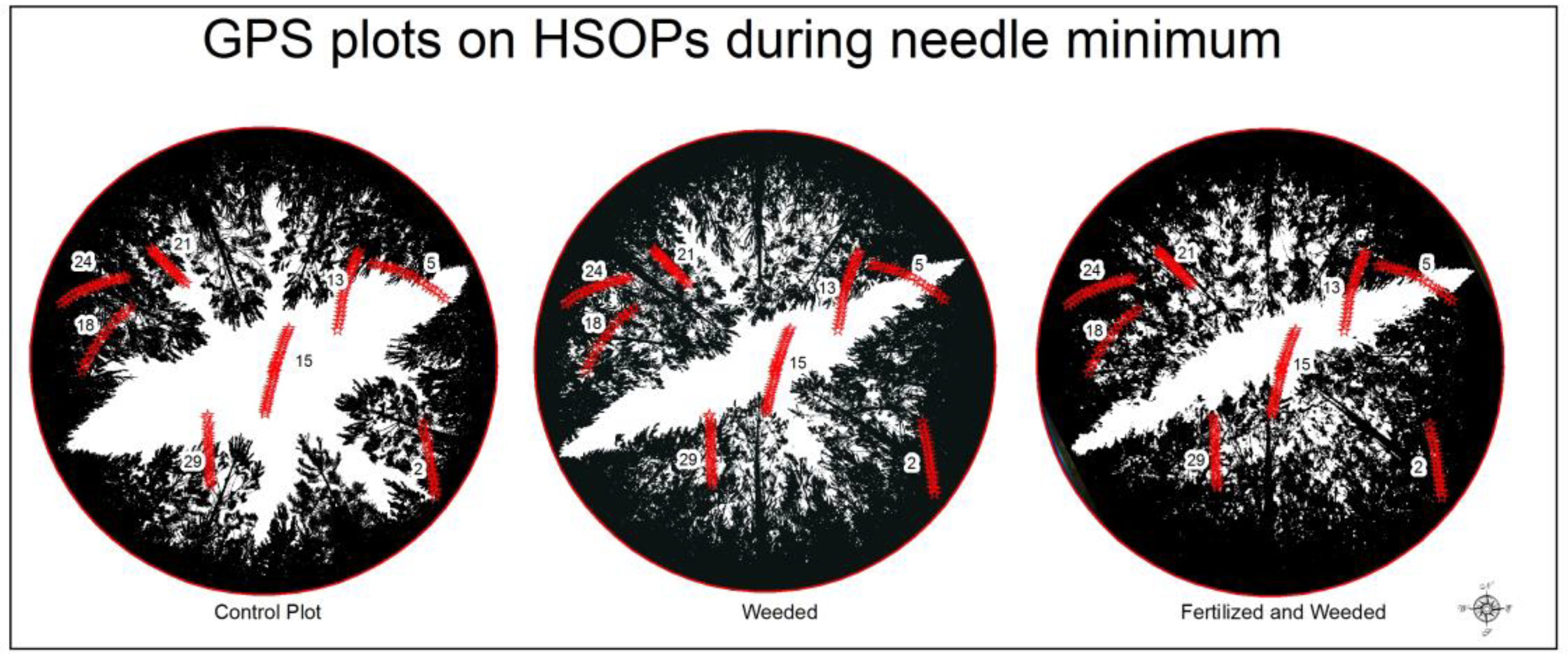
Figure 5.
The resulting binary images taken at the Intensive Management Practice Assessment Center managed forest taken during the needle maximum period with the GPS satellite vehicle positions (red circles) plotted inside the image.
Figure 5.
The resulting binary images taken at the Intensive Management Practice Assessment Center managed forest taken during the needle maximum period with the GPS satellite vehicle positions (red circles) plotted inside the image.

Figure 6.
The 1°-ringed hemispherical sky-oriented photo with a gray scale range of values associated with the canopy closure values. Dark colored rings indicate a high level of canopy closure and white rings indicate less forest media.
Figure 6.
The 1°-ringed hemispherical sky-oriented photo with a gray scale range of values associated with the canopy closure values. Dark colored rings indicate a high level of canopy closure and white rings indicate less forest media.


Table 1.
Forest study sites and description.
| ID | City Vicinity | Tree Type | Date (ddmmyy) | HT/STD (m) | DBH/STD (m) | Notes |
|---|---|---|---|---|---|---|
| 1 | West Point, NY | Oak/Hickory | 110515 | 23.4/3.4 | 0.30/0.18 | Military |
| 100% Deciduous | 100815 | Reservation | ||||
| 241015 | ||||||
| 170216 | ||||||
| 2 | IMPAC | 100% Pine | Managed Forest | |||
| Gainesville, FL | Control Plot | 110215/250815 | 5.77/1.4 | 0.09/0.05 | Fertilization | |
| Gainesville, FL | Weeded Plot | 110215/250815 | 8.21/0.64 | 0.12/0.04 | Research plots | |
| Fertilized and Weeded | 110215/250815 | 9.05/0.67 | 0.13/0.06 | |||
| 3 | Hogtown Forest | 80% Deciduous | 050216 | 20.4/2.47 | 0.46/0.08 | Uplands Natural Mixed Forest |
| Gainesville, FL | 20% Coniferous | Loblolly Woods Nature Park | ||||
| 4 | Charleston, SC | 90% Pine, 10% Deciduous | 230516 | 24.0/3.1 | 0.36/0.05 | Francis Marion National Forest |
| 5 | Alexandria, LA | 90% Pine, 10% Deciduous | 190616 | 23.2/4.1 | 0.56/0.11 | Kisatchie National Forest |
| 6 | Cold Spring, TX | 80% Pine, 20% Deciduous | 200616 | 19.5/4.7 | 0.52/0.13 | Sam Houston National Forest |
| 7 | Georgetown, TX | Ceder Elm and Live Oak with Ash Juniper | 220616 | 6.3/1.1 | 0.42/0.11 | North Fork of San Gabriel River |
| 8 | Cloudcroft, NM | Ponderosa Pine | 230616 | 23.3/3.2 | 0.41/0.12 | Lincoln National Forest |
| 9 | Flagstaff, AZ | Ponderosa Pine | 250616 | 19.2/6.8 | 0.41/0.07 | |
| 10 | Guadalupe, CA | Eucalyptus | 020716 | 28.2/3.3 | 0.42/0.14 | |
| 11 | San Luis Obispo | Agrifolia | 030716 | 6.9/1.5 | 0.22/0.09 | Military Base |
| 12 | Davenport, CA | 75% Redwood, 25% Douglas Fir and Tanoak | 050716 | 54.0/6.3 | 1.20/0.56 | California Polytechnic Research Center |
| 13 | Davenport, CA | 80% Tanoak, 25% Douglas Fir | 050716 | 18.7/1.4 | 0.28/0.08 | California Polytechnic Research Center |
| 14 | Tahoe NF | Ponderosa Pine | 070716 | 26.5/2.2 | 0.53/0.16 | University of California, Berkley Sagehen Experimental Forest |
| 15 | Nederland, CO | Aspen | 090716 | 8.4/2.6 | 0.20/0.06 |
Note: Where HT is Tree Height, DBH is Diameter at Breast Height and STD is Standard Deviation.
Table 2.
Canopy Closure Predictive Model Results with coefficients , and are in reference to Equation (3) and the root Mean Square Error (RMSE).
Table 2.
Canopy Closure Predictive Model Results with coefficients , and are in reference to Equation (3) and the root Mean Square Error (RMSE).
| ID | City Vicinity | a | B1 | B2 | RMSE | Adj R2 |
|---|---|---|---|---|---|---|
| 1 | West Point, NY | 18.85 | 7.79 | −5.53 | 3.28 | 0.60 |
| 2 | IMPAC | 19.32 | 7.79 | −5.49 | 2.78 | 0.71 |
| 3 | Hogtown Forest, Gainesville, FL | 25.05 | 5.26 | −6.02 | 3.02 | 0.66 |
| 4 | Charleston, SC | 27.87 | 4.25 | −7.00 | 3.10 | 0.64 |
| 5 | Alexandria, LA | 25.77 | 4.87 | −5.24 | 3.03 | 0.60 |
| 6 | Cold Spring, TX | 26.89 | 5.61 | −16.35 | 2.80 | 0.59 |
| 7 | Georgetown, TX | 23.94 | 6.25 | −8.02 | 3.71 | 0.61 |
| 8 | Cloudcroft, NM | 25.71 | 5.99 | −6.99 | 3.77 | 0.60 |
| 9 | Flagstaff, AZ | 21.70 | 6.70 | −0.50 | 3.33 | 0.57 |
| 10 | Guadalupe, CA | 28.83 | 5.08 | −8.81 | 2.66 | 0.66 |
| 11 | San Luis Obispo | 26.26 | 5.79 | −29.39 | 3.75 | 0.60 |
| 12 | Davenport, CA | 27.50 | 5.46 | −6.03 | 2.83 | 0.72 |
| 13 | Davenport, CA | 27.50 | 3.15 | −14.49 | 3.02 | 0.70 |
| 14 | Tahoe NF | 30.03 | 4.56 | −8.59 | 3.24 | 0.70 |
| 15 | Nederland, CO | 31.04 | 4.79 | −12.99 | 2.83 | 0.74 |
Table 3.
Absorption indexes of the forest study sites showing the results of the signal to noise forest index model (SFIM) and simplified signal to noise forest index model (SSFIM).
Table 3.
Absorption indexes of the forest study sites showing the results of the signal to noise forest index model (SFIM) and simplified signal to noise forest index model (SSFIM).
| ID | City Vicinity | Tree Type | HT/STD (m) | DBH/STD (m) | SNR Index (dB) SFIM | SNR Index (dB) SSFIM | |
|---|---|---|---|---|---|---|---|
| 1 | West Point, NY | Oak/Hickory | 23.4/3.4 | 0.30/0.18 | Fall | –3.74 | –3.75 |
| 100% Deciduous | Spring | –5.43 | –5.44 | ||||
| Summer | –5.54 | –5.55 | |||||
| Winter | –4.37 | –4.38 | |||||
| 2 | IMPAC | 100% Pine | |||||
| Gainesville, FL | Needle Minimum | See Table 1 | See Table 1 | –3.31 | –3.32 | ||
| Gainesville, FL | Needle Maximum | See Table 1 | See Table 1 | –4.30 | –4.31 | ||
| 3 | Hogtown Forest | 80% Deciduous | 20.4/2.47 | 0.46/0.08 | –5.87 | –5.89 | |
| Gainesville, FL | 20% Coniferous | ||||||
| 4 | Charleston, SC | 90% Pine, 10% Deciduous | 24.0/3.1 | 0.36/0.05 | –7.68 | –7.69 | |
| 5 | Alexandria, LA | 90% Pine, 10% Deciduous | 23.2/4.1 | 0.56/0.11 | –6.48 | –6.49 | |
| 6 | Cold Spring, TX | 80% Pine, 20% Deciduous | 19.5/4.7 | 0.52/0.13 | –6.03 | –6.06 | |
| 7 | Georgetown, TX | Cedar Elm and Live Oak with Ash Juniper | 6.3/1.1 | 0.42/0.11 | –5.15 | –5.16 | |
| 8 | Cloudcroft, NM | Ponderosa Pine | 23.3/3.2 | 0.41/0.12 | –3.12 | –3.12 | |
| 9 | Flagstaff, AZ | Ponderosa Pine | 19.2/6.8 | 0.41/0.07 | –2.83 | –3.35 | |
| 10 | Guadalupe, CA | Eucalyptus | 28.2/3.3 | 0.42/0.14 | –5.02 | –5.02 | |
| 11 | San Luis Obispo | Agrifolia | 6.0/1.5 | 0.22/0.09 | –3.10 | –3.11 | |
| 12 | Davenport, CA | 75% Redwood, 25% Douglas Fir and Tanoak | 54.0/6.3 | 1.20/0.56 | –10.78 | –10.80 | |
| 13 | Davenport, CA | 80% Tanoak, 25% Douglas Fir | 18.7/1.4 | 0.28/0.08 | –8.05 | –8.07 | |
| 14 | Tahoe NF | Ponderosa Pine | 26.5/2.2 | 0.53/0.16 | –3.98 | –3.98 | |
| 15 | Nederland, CO | Aspen | 8.4/2.6 | 0.20/0.06 | –4.99 | –5.00 | |
Note: Where HT is Tree Height, DBH is Diameter at Breast Height and STD is Standard Deviation.
© 2018 by the authors. Licensee MDPI, Basel, Switzerland. This article is an open access article distributed under the terms and conditions of the Creative Commons Attribution (CC BY) license (http://creativecommons.org/licenses/by/4.0/).
Share and Cite
MDPI and ACS Style
Wright, W.; Wilkinson, B.; Cropper, W., Jr. Development of a GPS Forest Signal Absorption Coefficient Index. Forests 2018, 9, 226. https://doi.org/10.3390/f9050226
AMA Style
Wright W, Wilkinson B, Cropper W Jr. Development of a GPS Forest Signal Absorption Coefficient Index. Forests. 2018; 9(5):226. https://doi.org/10.3390/f9050226
Chicago/Turabian StyleWright, William, Benjamin Wilkinson, and Wendell Cropper, Jr. 2018. "Development of a GPS Forest Signal Absorption Coefficient Index" Forests 9, no. 5: 226. https://doi.org/10.3390/f9050226
Note that from the first issue of 2016, this journal uses article numbers instead of page numbers. See further details here.