Effects of Plot Positioning Errors on the Optimality of Harvest Prescriptions When Spatial Forest Planning Relies on ALS Data

Abstract

Forest management planning is increasingly relying on airborne laser scanning (ALS) in forest inventory. The area-based method to interpret ALS data requires sample plots measured in the field. The aim of this study was to assess and trace the impacts of the positioning errors of field plots along the entire forest management planning process, from their effect on forest inventory results to the outcome of forest management planning. This research links plot positioning errors with the spatio-temporal allocation of forest treatments and calculates the inoptimality losses arising from plot positioning errors in ALS-based forest inventory. The study area was a forest management unit in Central Spain. Growing stock attributes were predicted for a grid of square-shaped cells. Alternative management schedules were simulated for the grid cells by using growth and yield models. Then, a spatial forest planning problem aiming at maximizing timber production with even-flow cuttings was formulated. Spatial objective variables were used to cluster management prescriptions into dynamic treatment units. We used simulated annealing to conduct spatial optimization. First, the true plot locations were used and then the whole process was repeated with normally distributed random errors with standard deviation equal to 2.5, 5 and 10 m, resulting in an average error of 1.47, 3.06 and 8.34 m, respectively. Increasing the level of positioning errors resulted in higher variability in the estimated growing stock attributes and in the achieved values of management goals. Sub-optimal prescriptions caused by the tested plot positioning errors caused up to 4.62% losses in timber production and up to 3.35% losses in utility. The losses increased with increasing plot positioning error.

1. Introduction

Spatial optimization in forest planning has been traditionally used to find approximate or exact solutions to complex spatial and combinatorial problems [1]. Creating dynamic treatment units along the forest planning horizon has been one of those spatially-explicit problems. In this approach, treatment units are created by aggregating small forest inventory units [2] considering both spatial and non-spatial goals in forest planning [3]. Dynamic treatment units evolve in time according to multiple management objectives and based on predicted stand dynamics and management prescriptions [4], starting from the present state. Therefore, the accuracy of the present state information based on forest inventory is crucial for the quality of forest management plans; inaccurate forest inventories may lead to non-optimal or illogical solutions of forest planning problems.

Nowadays, remote sensing (RS) is widely used to estimate growing stock attributes in forest inventory. Among the existing possibilities in RS-based forest inventory, airborne laser scanning (ALS) is an increasingly widespread measuring technique. The integration of the Global Positioning System (GPS) into forest inventory methods during the 1990s paved the way to the use of ALS to collect information about forests for management planning. Inference methods based on both georeferenced field plots and ALS data are usually followed by the area-based approach (ABA) to estimate growing stock attributes for a given area of interest [5]. The coordinates of field plot centres are used to extract ALS metrics for a given plot area and then, these metrics are used to model the relationships between ALS metrics and measured growing stock attributes. Plot-level models are applied over the entire inventory area resulting in a continuous coverage of predictions of growing stock attributes. In this process, several factors such as point density per area unit [6], size of the training plots [7] or sampling intensity [8] influence the accuracy of estimation models. Despite those factors, the ABA method usually produces satisfactory estimates for most of the growing stock attributes of interest used for forestry applications [9].

The accuracy of the ALS-based inventory depends also on the accuracy of the coordinates of field plots, which are typically measured with GPS devices. Forest cover and atmospheric disturbances influence on the quality and accuracy of GPS measurements [10] as they cause signal losses [11] resulting in biased tree estimates [12] depending on forest conditions and observation time among other factors. Previous studies have showed variation in plot positioning errors ranging from 2.5 m [10] to 5.6 m [13] or as much as 9.7 m [14]. Errors can be expected when reporting plot coordinates under canopy cover conditions [15,16] introducing errors in the subsequent steps of the inventory process [8]. Therefore, inoptimal decisions on forest treatments due to plot positioning errors might lead to losses in the achievement of forest management objectives, so-called inoptimality losses [17,18]. Previous research has addressed the financial consequences of uncertainty arising from forest inventory data [19] and from errors in growth predictions [20,21], but less attention has been paid to the effect of plot positioning errors on the type and location of treatment prescriptions in spatially explicit forest management planning. There are only a few cases [17,22] in which the effect of errors in ALS-based inventory has been analysed further than the forest inventory stage [23].

Assessing the effect of plot positioning errors throughout the spatial forest planning process is, therefore, a relevant topic as ALS-based forest inventories are increasingly used for forest planning purposes [5]. One of the reasons is the increasing capability of computational systems that makes it possible to obtain feasible dynamic treatment units while reducing the size of forest inventory units [24]. The aim of this study was to assess and trace the impact and propagation of plot positioning errors along the entire forest management planning process, by examining their influence on: (i) ALS-based estimates of growing stock attributes, (ii) location and type of management prescriptions obtained in spatial optimization, (iii) achievement of management objectives, (iv) degree of reliability of assigned prescriptions, and (v) inoptimality losses arising from an underachievement of forest management objectives due to plot positioning errors.

2. Materials and Methods

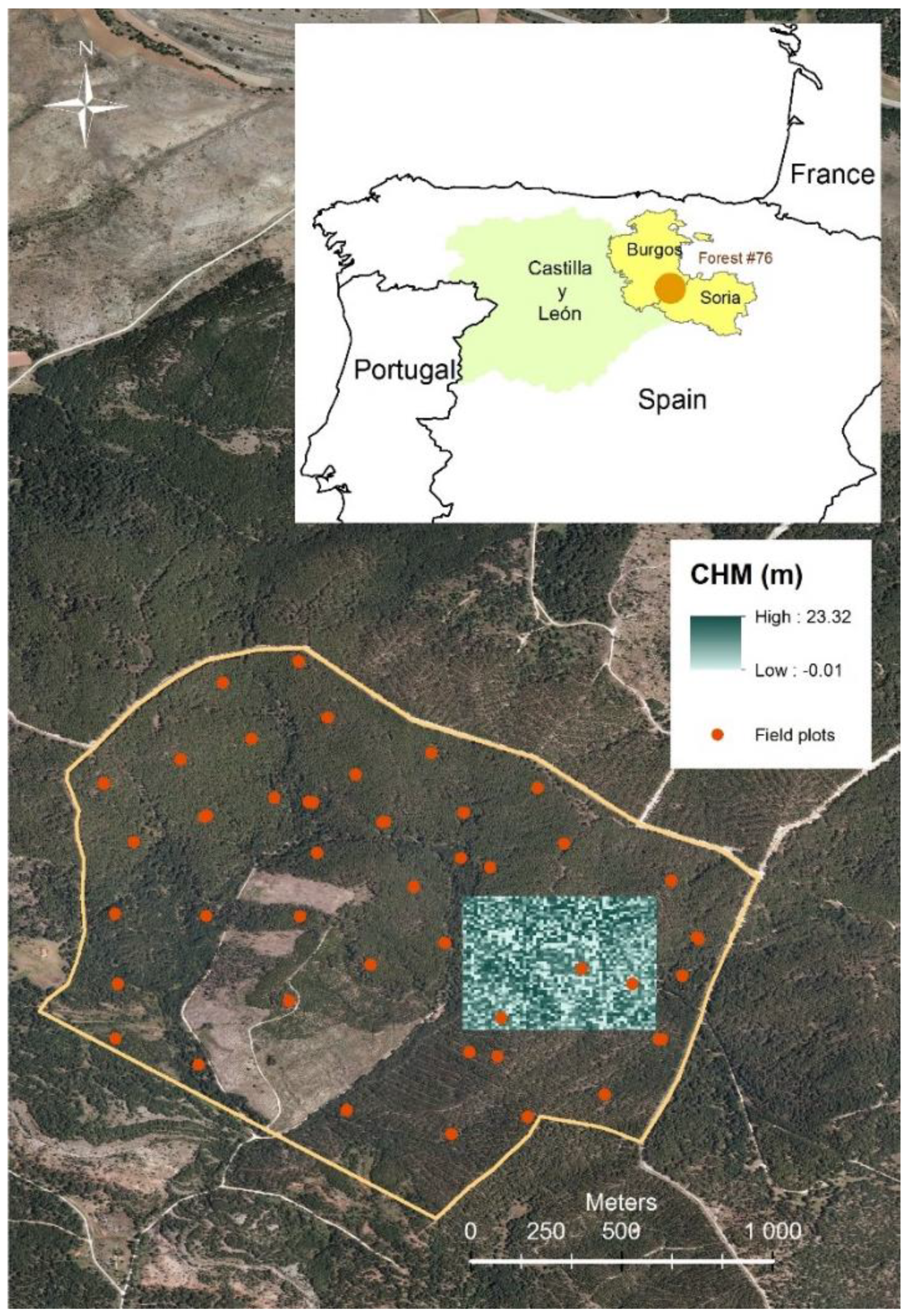
2.1. Study Area

The study area belongs to the municipality of San Leonardo de Yagüe, located in the forests of the Iberian Mountain System (Spain). The area selected for this study was 200.4 ha (UTM30N coordinates: 479,786-478,042 West-East; 4,635,486-4,633,630 South-North, 1122 m–1243 m a.s.l.), consisting of even-aged stands of Scots pine (Pinus sylvestris L.) and Maritime pine (Pinus pinaster Ait.). The understory was mainly composed of natural regeneration of pines and patches of Spanish oak (Quercus pyrenaica Willd.). The study area mainly includes dense forests that are managed using instructions for even-aged management. The effects of previous harvesting operations can be seen in the southern part of the area where scattered forest patches are surrounded by bare land (Figure 1). The forest area is a public forest owned by surrounding municipalities while forest management is carried out by regional forest service under the legislation of the regional government.

2.2. Data: Sample Plots and Laser Scanning Information

The experimental design was based on field sample plots (44) located across the study forest (Figure 1). Plots were circular with a fixed radius of 12.6 m and all the trees inside were measured. The location of plots aimed at covering the whole study area giving more importance to dense forest areas and area ignoring clear-cut areas. Neither pre- nor post-stratification of the sampling were proposed due to the small scale of the study forest. The field work was carried out during autumn 2010 using satellite positioning equipment (Trimble R6 Global Navigation Satellite System) to precisely locate the plot centre. The expected deviation between measured and real coordinates with the equipment used was less than one meter (0.25 m in X and 0.5 m in Y) and, for that reason, the stand-alone GPS method was used.

On each plot, all trees with diameter at breast height (dbh) > 10 cm were callipered and the heights (h) of all trees were measured using Vertex III hypsometer. Stand basal area (G) was computed by species as the sum of the individual-tree cross-sectional areas. Stand age was obtained by counting the annual growth rings of one dominant tree per plot. These variables, as well as stand density (N) and dominant height (H_o), were needed to simulate stand dynamics using growth and yield models. Information on the forest attributes measured from field plots is presented in

Table 1. Summary of field plot data.

Measured Variables	Min	Mean	Max
Diameter at breast height (cm)	10.0	28.7	55.7
Tree height (m)	7.1	14.8	22.0
Stand density (trees ha−1)	260.0	604.0	1080.0
Stand basal area (m2 ha−1)	21.2	47.4	72.1
Stand volume (m3 ha−1)	102.1	363.9	640.0
Dominant height (m)	11.9	17.3	21.8
Age (year)	33.0	56.4	74.0

.

Our georeferenced point cloud datasets were collected from the study area on 10 April 2010 using a Leica ALS60 II laser scanning system. The mean flight altitude was 2378 m, the scanning angle was 25° and the side overlap was 14% resulting in a nominal pulse density of 2 pulses m⁻². The accuracy was 0.13 m for the x and y coordinates and 0.08 m for the z coordinate. Both the first and the last return of laser pulse data were recorded. The approach described in [25] was used to classify echoes as ground and non-ground. An interpolated digital terrain model (DTM) of 1-m² cell size was created using ground echoes and the canopy height model (CHM) was created using the same cell size by searching the highest ALS echo from the centre of each cell within a radius of 1.6 m. Echoes for which the canopy height values were over 2 m above ground level were assumed to be vegetation hits (i.e., trees). Laser canopy heights above ground level were calculated by subtracting the DTM from ALS echoes.

2.3. Estimation of Forest Stand Attributes from ALS Data

We used an area-based approach [26] to model the relationships between ALS data and training data (ALS metrics and field sample plots) and predicted the growing stock attributes for the whole study area. In the first phase, the coordinates of plot centers were used as the centre of a circle (12.6 m radius) for which ALS metrics were computed. Using only the first echoes, percentiles of the height distribution of the pulse data (h₅, ..., h₁₀₀) and several other height metrics were computed for the plots, including the standard deviation of height echoes (h_Std), canopy relief ratio (CRR) and forest cover (FC₁). Forest cover was also computed considering all echoes (FC_All). All these metrics (more detailed description in [27]) were used as potential explanatory variables in the modelling of growing stock attributes.

Different methods have been previously applied to estimate growing stock attributes from ALS point clouds: linear regression analysis [28], k-nearest neighbor imputation [8] or linear mixed-effects modeling [29], among others. In our study, the forest planning system required the prediction of stand density (N), stand basal area (G) and dominant height (H_o) as well as the parameters of a diameter distribution model to transform the predictions of variables from plot/stand level to individual-tree level [4]. For each sample plot, the probability density function of the two-parameter truncated Weibull distribution was fitted based on dbh measurements using the maximum likelihood method [30]. Hereby, the parameters of the Weibull distribution were estimated.

We tested the possibility to predict simultaneously N, G and H_o from ALS metrics together with the b (location) and c (shape) parameters of Weibull diameter distribution from ALS-derived metrics using Seemingly Unrelated Regression (SUR) analysis [31]. Growing stock attributes measured in the field were also tested as potential predictors of Weibull parameters. Each of the five models was first fitted separately using stepwise regression analysis [32]. The stepwise procedure was used iteratively until all models had a maximum of three predictor variables, except the model for H_o, which had only one predictor based on the results of [33]. The final models were selected based on the following goodness-of-fit statistics: predictors’ significance, root mean square error (RMSE), degree of explained variance (R²), normality and homogeneity of variance of the residuals checked visually from Q–Q and scatter plots. Some of the selected predictors were present in more than one model. Statistical analysis was carried out using R software [34].

The preliminary model fitting tests revealed that SUR models for diameter distribution (Weibull parameters b and c) based on either ALS metrics or field plots measurements (i.e., measured growing stock attributes) were worse than the non-SUR models presented by [4] that used field plot measurements and plot altitude as predictors. Therefore, growing stock attributes N, G and H_o were predicted using the SUR method while Weibull parameters b and c were predicted using the existing models presented in [4], which in fact, were developed for a close study area of similar conditions.

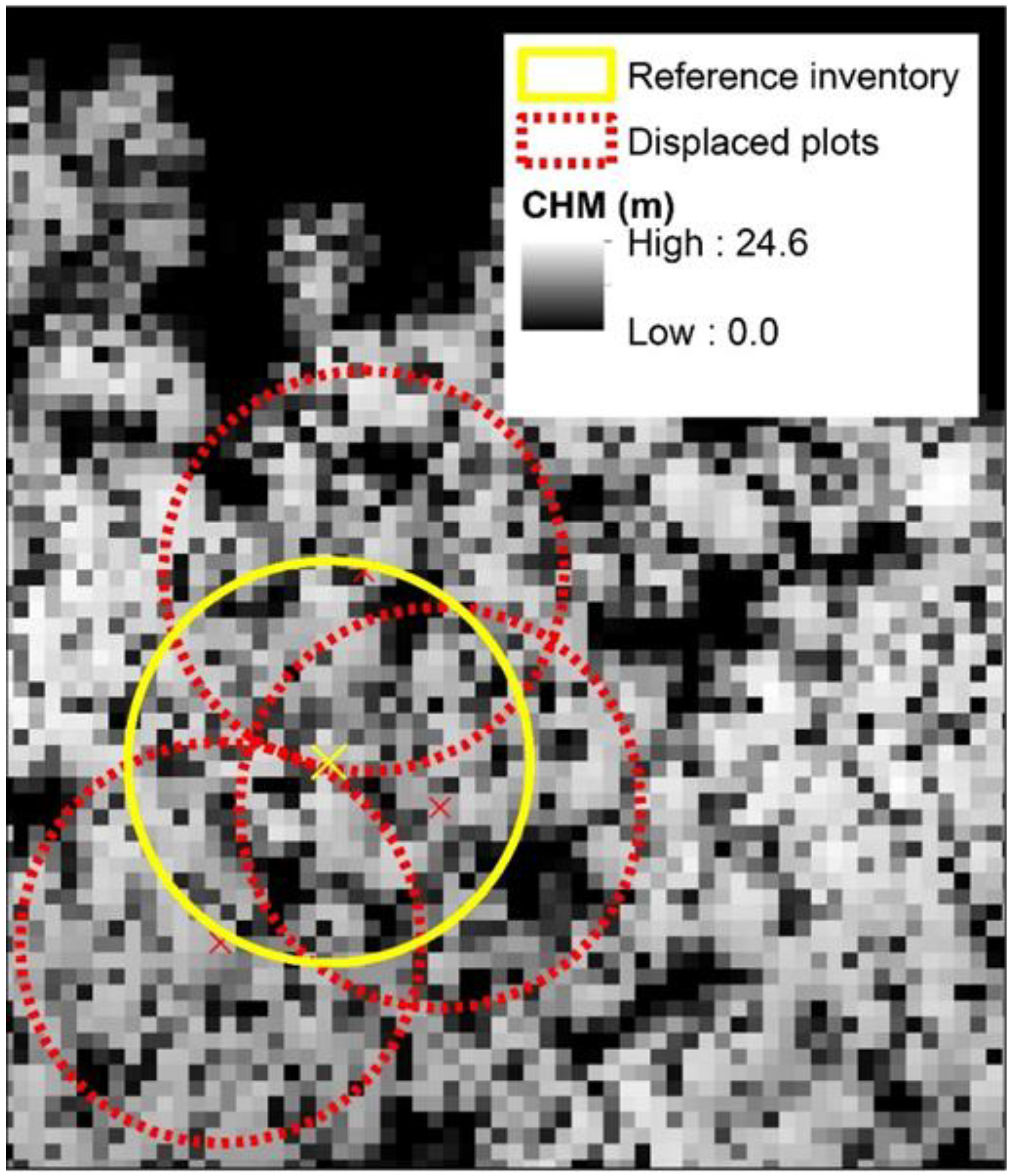
2.4. Simulating Plot Positioning Errors

We assumed the measured plot center positions to be true positions as the precision of the positioning equipment was less than a meter. With the purpose of analyzing the role of GPS precision, three alternatives were generated with normally distributed displacement errors [35]. The mean error was always zero and the standard deviation of errors was 2.5, 5 or 10 m. Random displacements corresponding to these standard deviations were drawn from normal distributions. The direction of the displacement was also random, uniformly distributed between 0 and 360°. This process was repeated 20 times for each of the three standard deviations, leading to 61 sets of plot locations including the original Reference inventory with no plot positioning errors (Figure 2). The means of the absolute values of simulated displacements with the standard deviations of 2.5, 5 and 10 m were 1.47, 3.06 and 8.34 m, respectively.

The predictors selected in model fitting when using Reference inventory data were also used in all replications containing positioning errors. Thus, ALS metrics were computed and models for growing stock characteristics were fitted independently for the 60 replications aiming at assessing the variation between repeated inventories, in addition to comparing the results with the estimates based on true plot positions. The models for growing stock variables were used as follows: the study area was gridded into a 0.05-ha-squared-shaped cells and ALS metrics for each cell were calculated as described above. Then, the set of models was applied over this grid to predict N, G and H_o for each cell. The parameters of the diameter distribution function were predicted from these variables.

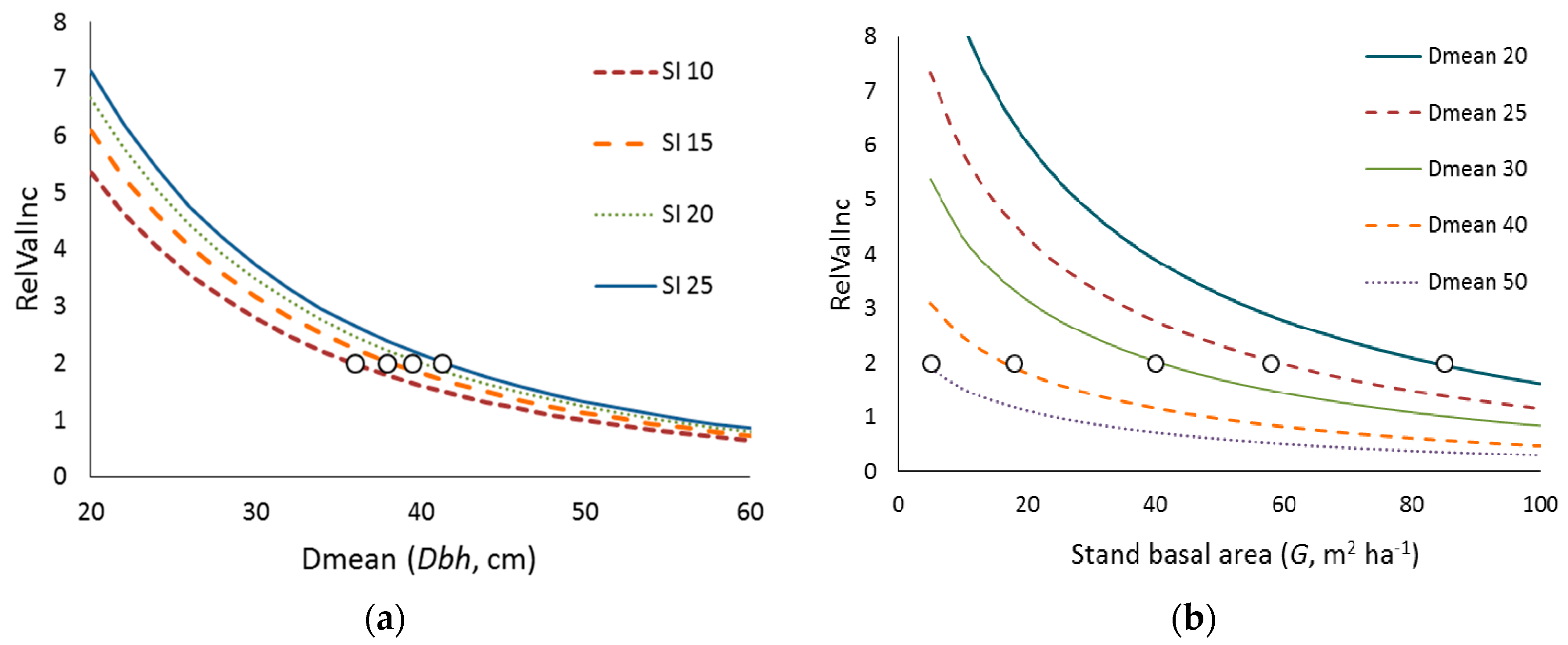
2.5. Developing Forest Management Rules and Creating Treatment Schedules

Simulation rules for economically optimal stand management (without considering forest level constraints) were developed as follows: the MONTE software [36,37] was used to calculate site index (SI), mean diameter (D_mean), stand basal area (G) and relative value increment (RelValInc) for a high number of forest inventory units. Those stand attributes were predicted from present state to 5 years ahead to calculate the relative value increment (i.e., we predicted 5-year value increment and divided it by the stumpage value of the stand). Then, a regression model showing RelValInc as a function of SI, G and D_mean was fitted to these data. This model was used to develop instructions for thinning basal area and for the diameter at which final felling should be done using 2% discount rate (Figure 3). When these rules are followed, trees are cut once RelValInc falls below 2%.

The forest management instructions were used as follows: if the D_mean of a given cell was higher than the final felling diameter of the instructions, seed tree cut was simulated followed by the removal of seed trees in the following 10-year period. Otherwise, G was compared to the thinning basal area (i.e., G at which thinning is proposed for a certain SI according to the instructions), and thinning treatments were simulated if G was higher than the thinning basal area. To generate several treatment alternatives for each calculation unit, final felling diameter and thinning basal area values of the management instructions were multiplied by three constants: 0.7, 1.0 and 1.3. Moreover, three thinning intensities were simulated: light (21% reduction in stand basal area), moderate (30%) and heavy thinning (39%). Each combination was applied with 8 different settings concerning whether cutting was allowed or not during a certain 10-year period (from 000 = no cuttings to 111 = cutting allowed during every period). Overall, 216 simulations were done for each calculation unit, resulting in 864,864 schedules for all calculation units for the three 10-year periods composing the forest plan.

2.6. Planning Problem Formulation

We formulated a spatially explicit forest planning problem that was applied to all 61 inventory datasets (Reference inventory and 60 inventories with simulated plot positioning errors). Overall, 61 forest management plans were compiled for three 10-year periods, all aiming at maximising both timber production (sum of harvested volumes and the standing volume at the end of the third 10-year period) and the spatio-temporal clustering of management prescriptions under the constraint of even-flow of cuttings. A utility function including the following spatial and non-spatial objectives was maximized:

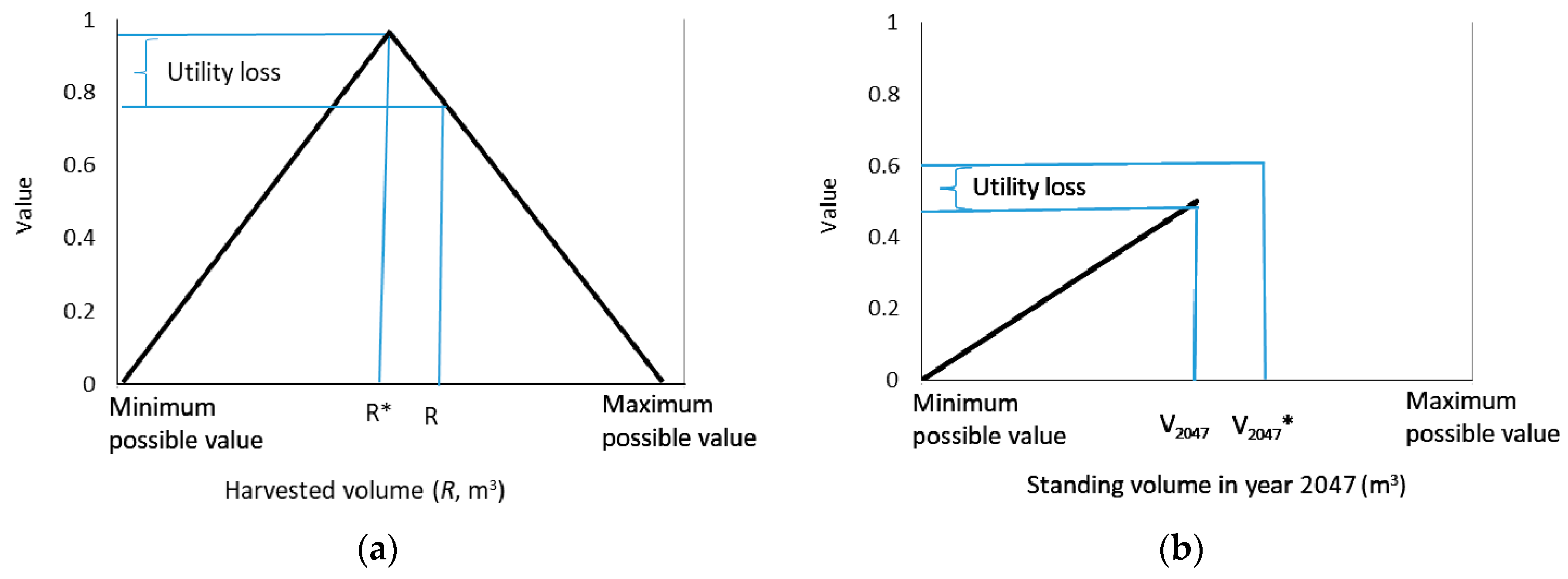
• Maximization of the growing stock volume at the end of the plan (V₂₀₄₇, m³).
• Removal of 7500 m³ during each 10-year period (R₁, R₂, R₃, m³).
• Maximization of the proportion of cut–cut borders of adjacent cells (CC).
• Maximization of the proportion of cut–cut borders of adjacent cells that are prescribed as final felling (CC_FF).
• Minimization of the proportion of cut–non-cut borders of adjacent cells (CNC).
• Minimization of the proportion of cut–non-cut borders of adjacent cells that are prescribed as final felling (CNC_FF).

Aggregated harvest blocks were pursued via spatial objectives: CC and CNC variables aimed at aggregating all cuttings while CC_FF and CNC_FF specifically aggregated final fellings to prevent isolated segments prescribed as final felling from appearing within a thinning block. In this way, compact and round-shaped treatment units could be achieved [4].

The above-described management objectives were expressed as an additive utility function (Equation (1)), which was the objective function (OF) of the optimization problems. Each management objective has an associated sub-utility function that scales all variables to the same range [0–1] and converts the quantity of an objective variable into utility. Single-objective optimizations were carried out to calculate the maximum possible value for each objective variable and the minimum value for growing stock volume in year 2047. Then, preliminary optimizations were used to set the weights, giving much importance to CNC and CNC_FF so as to reduce isolated treated cells and obtain a layout consisting of compact harvest blocks. The final OF was as follows:

$$\begin{array}{r}OF=0.18 \left(\frac{V_{2047}-V_{min}}{V_{\max }}\right)+0.09 u_{1 }\left(R_1\right)+0.09 u_2 \left(R_2\right)+0.09 u_3\left(R_3\right)+0.04\left(\frac{CC}{Max CC}\right)\\ +0.235\left(1-\frac{CNC}{Max CNC}\right)+0.04 \left(\frac{C{C}_{FF}}{Max C{C}_{FF}}\right)+0.235\left(1-\frac{CN{C}_{FF}}{Max CN{C}_{FF}} \right)\end{array}$$

(1)

where V_max and V_min are the largest and smallest ending volume for the whole forest after 30 years (m³), u_i is the sub-utility function for harvested volume during period i while Max CC, Max CNC, Max CC_FF, and Max CNC_FF are the values of the spatial objective variables in the preliminary single-objective optimizations. The shape of the sub-utility functions used in Equation (1) for harvested volumes is shown in Figure 4.

2.7. Spatial Optimization

Simulated annealing (SA) heuristic was used to maximize the OF for all 61 forest plans. There is a wealth literature on the good performance of SA to tackle different types of forest planning problems [38] and more specifically, to create harvest blocks [4]. Most heuristic methods first generate an initial solution that is gradually improved by making local changes (moves). In our study, a move involved the reassignment of a management prescription of two cells at the same time. Moves (changes) were made to the initial solution by selecting first a random pair of cells and then a random schedule for these two cells from those produced beforehand. The schedule for each cell that was currently in the solution was replaced by the randomly selected alternative schedule. The move was accepted if the OF value improved; otherwise, it was accepted with the following probability:

$$p=exp{ }^{\frac{\left(O{F}_{Candidate}-O{F}_{Current}\right)}{T }}$$

(2)

where OF_Current is the OF value of the solution before implementing the move, OF_Candidate is the OF value after the move, and T is ‘temperature’ which affects the probability of accepting candidate solutions poorer than the current solution. The temperature was decreased toward the end of the search, which means that the probability to accept inferior moves also decreased. Several candidate moves were produced at each temperature. Apart from temperature, other parameters [39] and stopping criteria [40] control the performance of SA. Tests with the Reference inventory were used to adjust the control parameters. The following values were used: 2.5 × 10⁻⁵ for initial temperature, 0.92 for lowering the temperature during the search, 10–13 for freezing temperature while the number of candidate solutions evaluated in each temperature was 400. The intrinsic variability of using heuristic-based optimization was assessed by repeating the optimization 10 times using Reference inventory. The run with the highest utility was used to measure the deviation of management objectives in forest plans containing positioning errors (60).

2.8. Achievement of Forest Management Objectives and Inoptimality Losses

The consequences of applying wrong decisions based on erroneous data as compared to the use of more accurate information may result in inoptimality losses. For the assessment of inoptimality losses, the optimal solutions for the 60 “wrong” forest inventories containing plot positioning errors were used with the Reference inventory data. Inoptimality losses were then calculated in terms of timber production (P_l, sum of V₂₀₄₇ and periodical cuttings less initial volume) and utility (U_l; i.e., the value of the OF, calculated with Equation (1)) as follows:

$$P_l= \frac{\left(P^{Ref}- \frac{{{\displaystyle \sum }}_{i=1}^{20}{P}_i{}^{Err} }{20}\right)}{P^{Ref}}$$

(3)

$$U_l= \frac{\left(U^{Ref}- \frac{{{\displaystyle \sum }}_{i=1}^{20}{U}_i{}^{Err} }{20}\right)}{U^{Ref}}$$

(4)

where P^Ref and U^Ref are the total timber production and utility when using Reference inventory data with its spatial and temporal allocation of forest treatments, while P_i^Err and U_i^Err correspond to total production and utility in replication i as a result of using the “wrong” solution of replication i on the Reference inventory data (Figure 4).

3. Results

3.1. Impact of Plot Positioning Errors on the Estimated Stand Attributes

The predictors selected through stepwise model fitting procedure were FC₁, CRR and h_Std for stand density (N), FC₁, h₂₀ and FC_All for stand basal area (G), and h₉₅ for dominant height (H_o). The fitting statistics showed poorer estimation of forest attributes, more clearly for N and G, when the plot positioning error increased (

Table 2. Effect of plot positioning errors on the estimation of stand variables as described by root mean squared error (RMSE %) and adjusted R², both computed on the original scale.

Displacement	Stand Density Model (Tree ha−1)		Stand Basal Area Model (m2 ha−1)		Dominant Height Model (m)
	RMSE (%)	R2	RMSE (%)	R2	RMSE (%)	R2
Reference	25.6	0.56	14.6	0.85	4.6	0.91
2.5 m	26.9	0.47	15.3	0.82	4.6	0.91
5 m	28.8	0.39	16.2	0.80	4.9	0.90
10 m	30.9	0.31	18.6	0.73	6.9	0.85

). Thus, the proportion of explained variance (R²) decreased progressively from 0.56 (for N), 0.85 (G) and 0.91 (H_o) down to 0.31 (N), 0.73 (G) and 0.85 (H_o), when the standard deviation of plot positioning error increased from zero to 10 m.

We observed increasing overestimation of present state information with increasing plot positioning errors (

Table 3. Effect of plot positioning errors on the prediction of growing stock attributes. Mean values and standard deviations (Std) among replications were calculated using the 60 datasets containing positioning errors. For the case of stand density (N) and stand basal area (G), the standard deviation between cells was also computed (Std_cells).

Displacement	N Predictions (Tree ha−1)			G Predictions (m2 ha−1)			V Predictions (m3 ha−1)
	Mean	Std	Stdcells	Mean	Std	Stdcells	Mean	Std
Reference	546.5	-	298.6	34.9	-	20.4	345.1	-
2.5 m	549.6	11.5	291.7	34.8	0.1	20.2	345.2	4.0
5 m	562.9	22.5	278.9	35.2	0.4	19.9	348.3	6.8
10 m	626.9	57.9	261.1	36.5	1.2	18.5	361.4	10.5

). The overestimation in total growing stock volume reached 4.7% for the maximum standard deviation of displacements tested (10 m). The between-cell standard deviation of predicted N and G tended to decrease with increasing plot positioning error, resulting in increasing “homogenization” of the predicted forest structure throughout the study area due to the averaging effect in the prediction of stand characteristics when models were fitted to data containing plot positioning errors.

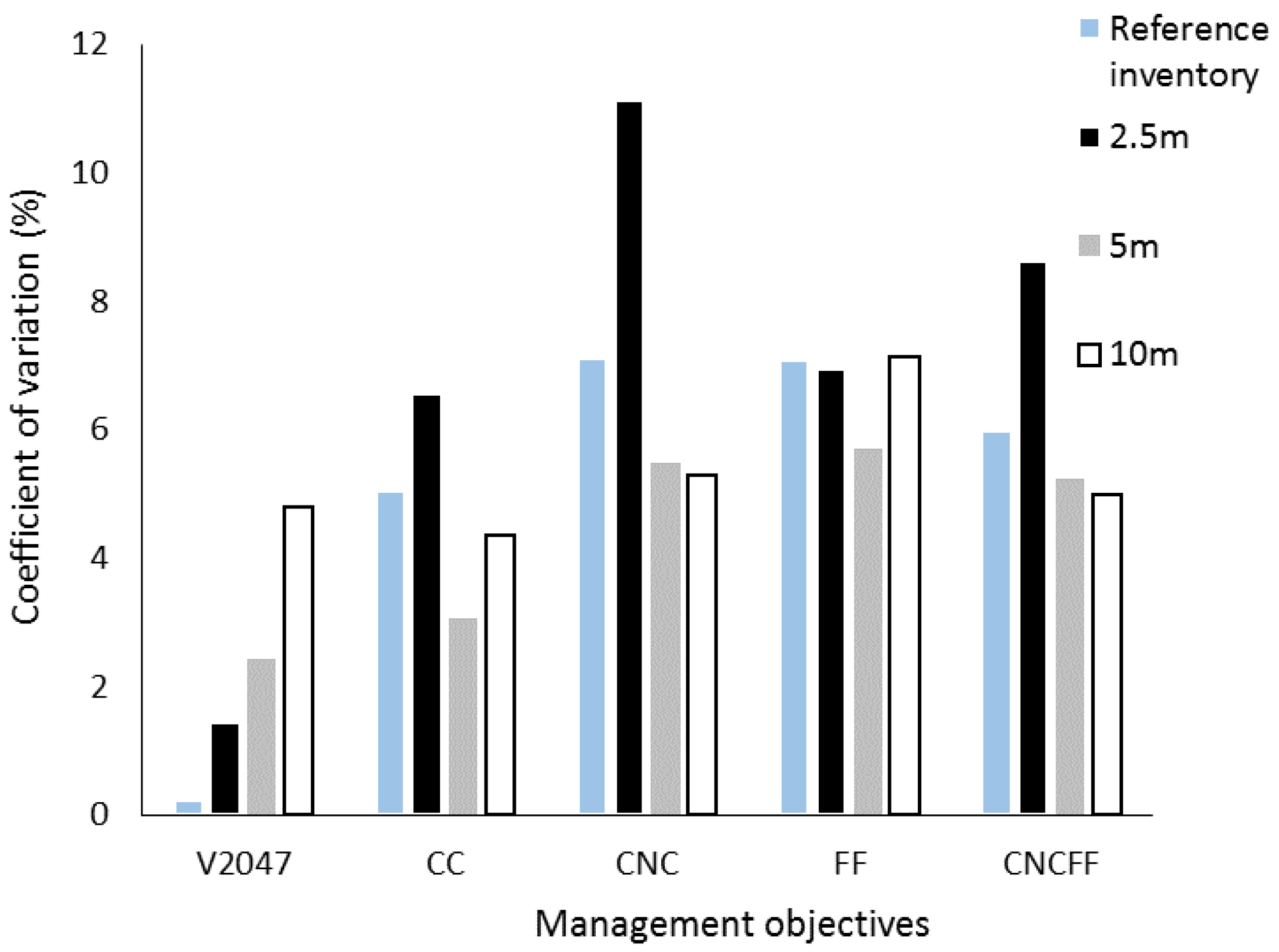
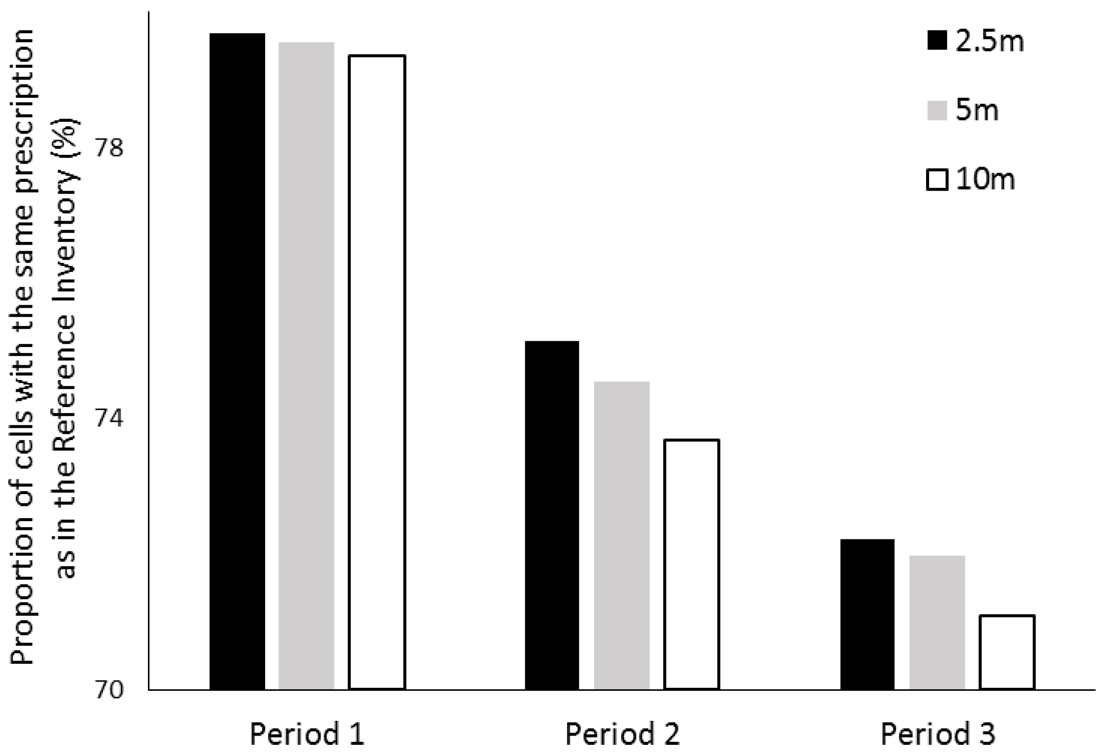
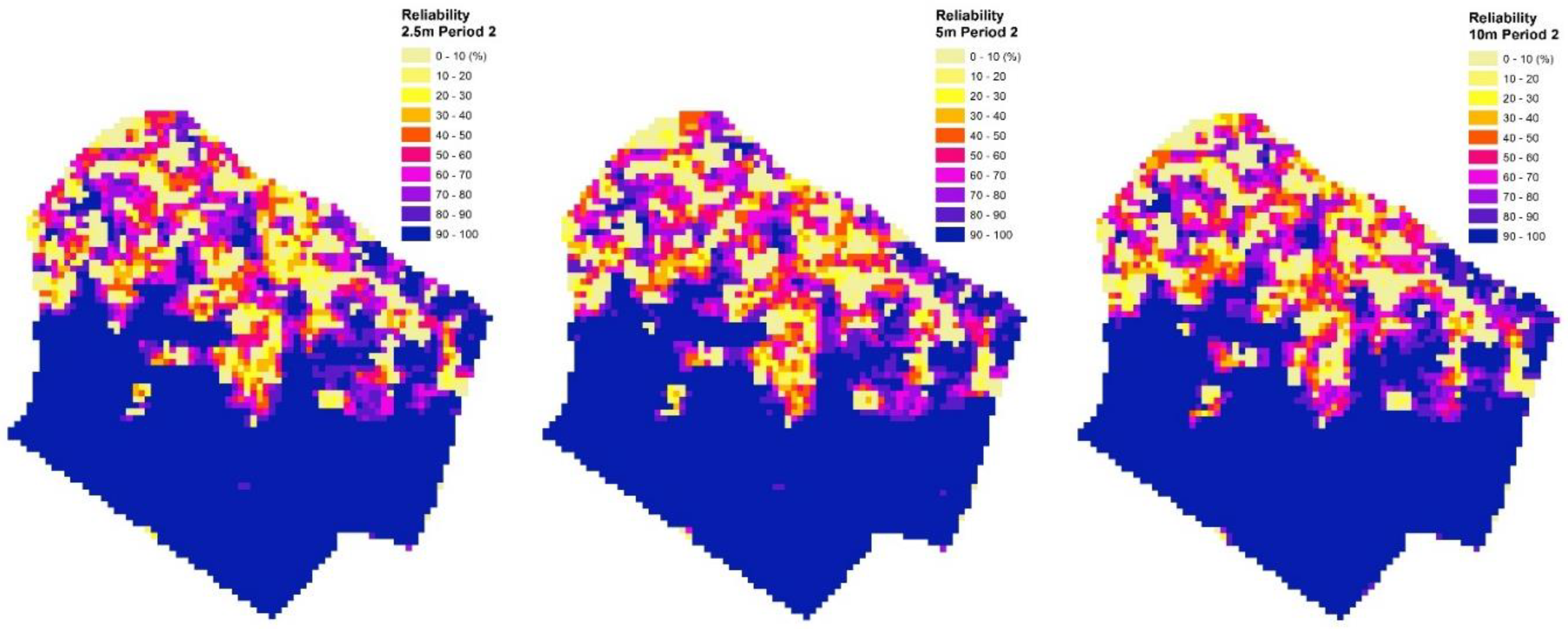
3.2. Impact of Plot Positioning Errors on Forest Management Goals and Prescriptions

Repeating the optimization run with the error-free dataset showed slight variation in the achievement of non-spatial goals (harvesting targets R₁, R₂, R₃ were always met). The coefficient of variation of V₂₀₄₇ (CV, standard deviation divided by the computed average value) was only 0.24%, substantially lower than in the presence of positioning errors: 1.44, 2.44 and 4.81%, respectively, for 2.5-, 5- and 10-m standard deviations of displacements (Figure 5). However, corresponding differences in CV were not observed for the case of spatial objective variables.

The area devoted to thinning and final felling prescriptions was quite similar in the plan based on the Reference inventory (thinning 51.6 ha and final felling 47.4 ha). Plot positioning errors caused a minor reduction in the area of final fellings: the mean areas of final fellings were 51.5, 50.6 and 49.5 ha for 2.5-, 5- and 10-m displacement, respectively. The thinning areas were 46.5, 48.9 and 48.7 ha, respectively. Although the mean values were very similar in all cases, we observed increasing variability between repeated inventories and optimizations with increasing plot positioning error.

The reliability assessment (Figure 6) showed that 75.7, 75.4 and 74.7% of all prescriptions, including no-treatment, were assigned in the same way as in the Reference inventory for the case of 2.5-, 5- and 10-m standard deviation of displacements, respectively. These percentages decreased from Period 1 to Period 3. The spatial layout of the reliability maps of prescriptions did not show any clear trends which could be attributed to the accuracy level of plot positioning (Figure 7). The clustering of prescriptions in the northern part reflects the distribution of age classes in Forest #76: mature and dense forests are located in the north part while both young stands and the clear-cut area can be identified (Figure 1) in the south part.

3.3. Inoptimality: Utility and Yield Losses

Using the management prescriptions resulting from optimizations with the datasets containing plot positioning errors with the Reference inventory data led to decreased growing stock volume at the end of the plan (V₂₀₄₇) and increased total cuttings in all periods (

Table 4. Effect of applying the optimization solutions based on inaccurate forest inventory data to Reference inventory data in terms of ending volume (V₂₀₄₇) and periodical cutting volumes (R₁, R₂, R₃). The results show the mean value of 20 replications for each displacement distance. Inoptimality losses in utility and in timber production (Prod loss) are also presented.

	V2047 (m3 103)	R1 (m3)	R2 (m3)	R3 (m3)	Prod Loss (m3)	Prod Loss (%)	Total Utility	Utility Loss (%)
Reference	55.25	7500	7500	7500		-	0.885	-
2.5 m	54.01	7818	7937	7950	36	0.42	0.860	2.82
5 m	53.71	7887	8005	8076	109	1.26	0.858	2.99
10 m	53.61	7816	7888	8009	406	4.68	0.855	3.35

). As a result, the average timber production loss (Equation (3)) was 0.42, 1.26 and 4.68% for 2.5-, 5- and 10-m standard deviations of displacements, respectively. The mean utility loss (Equation (4)) among the replications ranged from 2.82 to 3.35% with increasing plot positioning error. The maximum utility loss observed among individual replications was 5.79%.

4. Discussion

4.1. Effect of Plot Positioning Errors on the Estimation of Growing Stock Attributes

The effect of plot positioning errors on the estimation of growing stock attributes was considerable, as described by increasing RMSE with increasing positioning error. In this regard, our findings are in accordance with previous studies on the effect of plot positioning errors on ALS-based estimations [23] and the effect of co-registration error on the estimation of ALS metrics [7]. The applied SUR method resulted in better fitting statistics than those reported in previous research for the same study area [33]. For the case of diameter distribution models, our results showed that predictions based on ALS data were slightly less reliable than the diameter distribution models published by [4] based on growing attributes retrieved from field measurements only. In the absence of existing models, the SUR method is a reliable method to simultaneously predict several growing stock attributes of interest [31].

Increasing plot positioning error resulted in the prediction of more homogeneous forest structure throughout the study area. This is explained by the fact that, in the simulated positioning errors, ALS metrics were not calculated from the area actually covered by the field inventory plots. Consequently, the correlations between ALS metrics and stand attributes were weaker leading to flatter models. The mean computed values for the predicted growing stock attributes reflected the overestimation caused by plot positioning errors in ALS-based forest inventory. This overestimation might be explained by plot locations and study area conditions: as a result of the systematic sampling design, most of the plots were placed in dense mature stands and just a few of them were located on transitional areas between different types of forest structure.

Compared to our results for this case study area, positioning errors in more heterogeneous and fragmented forests may result in greater discrepancies between the solutions achieved for the Reference inventory (error-free dataset) and for inventories containing positioning errors. Therefore, the difference between Reference inventory and the displaced datasets might increase in other forest ecosystems. In addition, the reported sub-metric precision of the positioning equipment used in our study did not guarantee that greater positioning errors never occurred. Since the plot coordinates in Reference inventory may also contain errors, our calculations on the effects of plot positioning errors may underestimate the true effect of positioning errors.

The performance and efficiency of GPS equipment in the field is highly dependent on forest cover [11]. Therefore, computing ALS statistics for plot coordinates but also including plot surroundings may be a good strategy to classify ALS statistics and select those which show less variation (i.e., less sensitive to plot positioning errors). In this way, the modelling of growing stock attributes could implicitly account for the presence of positioning errors by gathering information of surrounding areas for a robust selection of model predictors. Increasing the size of sample plots also contributes to reducing the uncertainty when computing ALS statistics as previous literature showed [23].

4.2. Effect of Plot Positioning Errors on Decision-Making in Forest Planning

Regarding the impact of plot positioning errors on the delineation of dynamic treatment units and the spatio-temporal allocation of management prescriptions, we found a slight reduction of final fellings with increasing plot positioning error, which is in line with previous research [41]. Final fellings are prescribed in mature stands, where the mean tree diameter is high. Because of the aforesaid homogenization of the estimated stand structure, the mean diameter of the most mature stands is underestimated. Thus, many cells that could have been scheduled for final fellings in the absence of plot positioning errors were scheduled for thinnings when positioning errors were introduced. The spatial distribution of growing stock attributes represents, together with the management objectives, the driving force in any forest management plan in any area. In this regard, the effect of positioning errors when assigning prescriptions is likely to be reinforced by the study area conditions and so, the proportion of cells close to the eligibility criteria. Further research is needed to evaluate, e.g., the influence of management intensity and sampling design on the outcome of forest plans considering the presence of plot positioning errors.

Our results are in line with previous research by [17] who suggested that inventory errors may cause a decline in timber production due to inaccurate inventory data. The increment of treated area as a consequence of forest inventory errors (but different from plot positioning errors) was observed by [22], but not in our case, although we found increasing variability as a consequence of increasing displacement. The small effect of plot positioning errors might be due to the homogeneity of the forest in places where plots were measured, which means that it did not matter much if the growing stock attributes were measured in the right or slightly displaced location. Increasing harvesting targets would have resulted in a higher number of prescription with a higher impact of plot positioning errors. However, the harvested volume of this study was close to the net increment in growing stock volume, which means that the results of this study correspond to a normal management of forests devoted to sustainable timber production.

The behavior of preliminary optimizations with the error-free dataset showed that heuristic SA-based optimization made it difficult to detect systematic effects of plot positioning errors on spatial objective variables. This is because a certain harvested volume could be allocated to the cells in many different ways, all of which are nearly equally good in terms of utility. As a result, the impact of positioning errors on the reliability of prescriptions at certain locations of a rather homogeneous forest was difficult to see. The impact of positioning errors on forest management planning might be stronger in forest management units characterized by more heterogeneous stand structures and more fragmentation across the area. Variation in inoptimality losses when using ALS-based forest inventory might be explained by stage of forest development or site classes [21]. Further research in other study areas and using alternative ALS-based forest inventory approaches [42] may contribute to deepening our knowledge of the impact of plot positioning errors throughout the forest management planning process, since previous research has not thoroughly addressed this question. Indeed, previous studies on the effect of forest inventory errors on forest management planning [22] did not explicitly consider errors arising from the uncertainty in plot positioning due to limited GPS accuracy. Yet, previous research supports our results inasmuch as forest inventory errors other than plot positioning inaccuracy were also reported to modify the spatio-temporal allocation of forest treatments [19,20].

5. Conclusions

In this study, we analyzed and traced the influence of plot positioning errors from the forest inventory phase to the decision-making stage in optimal forest management planning. Our study links errors in plot positioning with their impact on the spatio-temporal allocation of forest treatments in the context of dynamic treatment units, and calculates the resulting inoptimality losses. Taking into account that the differences in terms on utility and timber production between 0-, 2.5- and 5-m standard deviations of displacement error were very small and that the average timber production loss with 10 m standard deviation was only 406 m³ in 30 years in a 200-ha forest, the use of very accurate but very expensive GPS devices may not be worthwhile when conducting ABA as described in this study. However, further analyses on the influence of sampling designs [41], structure of the forest and management goals are needed in order to generalize our findings.

References

1. Baskent, E.Z.; Keles, S. Spatial forest planning: A review. Ecol. Model. 2005, 188, 145–173. [Google Scholar] [CrossRef]
2. Öhman, K.; Eriksson, L.O. Aggregating harvest activities in long term forest planning by minimizing harvest area perimeters. Silva Fenn. 2010, 44, 77–89. [Google Scholar] [CrossRef]
3. Weintraub, A.; Murray, A.T. Review of combinatorial problems induced by spatial forest harvesting planning. Discret. Appl. Math. 2006, 154, 867–879. [Google Scholar] [CrossRef]
4. Pascual, A.; Pukkala, T.; Rodríguez, F.; de-Miguel, S. Using spatial optimization to create dynamic forest treatment units from small interpretation units of LiDAR inventory. Forests 2016, 7, 220. [Google Scholar] [CrossRef]
5. Vauhkonen, J.; Maltamo, M.; McRoberts, R.E.; Næsset, E. Introduction to Forestry Applications of Airborne Laser Scanning. In Forestry Applications of Airborne Laser Scanning: Concepts and Case Studies; Maltamo, M., Ed.; Managing Forest Ecosystems; Springer: Dordrecht, The Netherlands, 2014. [Google Scholar]
6. Næsset, E. Effects of different sensors, flying altitudes, and pulse repetition frequencies on forest canopy metrics and biophysical stand properties derived from small-footprint airborne laser data. Remote Sens. Environ. 2009, 113, 148–159. [Google Scholar] [CrossRef]
7. Frazer, G.W.; Magnussen, S.; Wulder, M.A.; Niemann, K.O. Simulated impact of sample plot size and co-registration error on the accuracy and uncertainty of LiDAR-derived estimates of forest stand biomass. Remote Sens. Environ. 2011, 115, 636–649. [Google Scholar] [CrossRef]
8. Maltamo, M.; Bollandsas, O.M.; Naesset, E.; Gobakken, T.; Packalen, P. Different plot selection strategies for field training data in ALS-assisted forest inventory. Forestry 2010, 84, 23–31. [Google Scholar] [CrossRef] [Green Version]
9. Holmgren, J. Prediction of tree height, basal area and stem volume using airborne laser scanning. Scan. J. For. Res. 2004, 19, 543–553. [Google Scholar] [CrossRef]
10. Sigrist, P.; Coppin, P.; Hermy, P. Impact of forest canopy on quality and accuracy of GPS measurements. Int. J. Remote Sens. 1999, 20, 3595–3610. [Google Scholar] [CrossRef]
11. Hasegawa, H.; Yoshimura, T. Estimation of GPS positional accuracy under different forest conditions using signal interruption probability. J. For. Res. 2008, 12, 1–7. [Google Scholar] [CrossRef]
12. Mauro, F.; Valbuena, R.; Manzanera, J.; García-Abril, A. Influence of Global Navigation Satellite System errors in positioning inventory plots for tree-height distribution studies. Can. J. For. Res. 2011, 41, 11–23. [Google Scholar] [CrossRef]
13. Næsset, E.; Jonmeister, T. Assessing point accuracy of DGPS under forest canopy before data acquisition, in the field, and after postprocessing. Scan. J. For. Res. 2002, 17, 351–358. [Google Scholar] [CrossRef]
14. Camp, M.J.; Rachlow, J.L.; Cisneros, R.; Roon, D.; Camp, R.J. Evaluation of Global Positioning System telemetry collar performance in the tropical Andes of southern Ecuador. Natureza Conservação 2016, 14, 128–131. [Google Scholar] [CrossRef]
15. Johnson, C.E.; Barton, C.C. Where in the world are my field plots? Using GPS effectively in environmental field studies. Front. Ecol. Environ. 2004, 2, 475–482. [Google Scholar] [CrossRef]
16. Wing, M.G.; Karsky, R. Standard and real-time accuracy and reliability of a mapping-grade GPS in a coniferous western Oregon forest. West. J. Appl. For. 2006, 21, 222–227. [Google Scholar] [CrossRef]
17. Eid, T. Use of uncertain inventory data in forestry scenario models and consequential incorrect harvest decisions. Silva Fenn. 2000, 34, 89–100. [Google Scholar] [CrossRef]
18. Holmgren, P.; Thuresson, T.; Holmgren, P.; Thuresson, T. Applying Objectively Estimated and Spatially Continuous Forest Parameters in Tactical Planning to Obtain Dynamic Treatment Units. For. Sci. 1997, 43, 317–326. [Google Scholar]
19. Holopainen, M.; Mäkinen, A.; Rasinmäki, J.; Hyytiäinen, K.; Bayazidi, S.; Piëtila, I. Comparison of various sources of uncertainity in stand-level present value estimates. For. Pol. Econ. 2010, 12, 377–386. [Google Scholar] [CrossRef]
20. Mäkinen, A. Uncertainty in Forest Simulators and Forest Planning Systems. Ph.D. Thesis, University of Helsinki, Helsinki, Finland, 2010. [Google Scholar]
21. Pietilä, I.; Kangas, A.; Mäkinen, A.; Mehtätalo, L. Influence of growth prediction errors on the expected losses from forest decisions. Silva Fenn. 2010, 44, 829–843. [Google Scholar] [CrossRef]
22. Islam, M.N.; Pukkala, T.; Kurttila, M.; Mehtätalo, L.; Heinonen, T. Effects of forest inventory errors on the area and spatial layout of harvest blocks. Eur. J. For. Res. 2012, 131, 1943–1955. [Google Scholar] [CrossRef]
23. Gobakken, T.; Næsset, E. Assessing effects of positioning errors and sample plot size on biophysical stand properties derived from airborne laser scanner data. Can. J. For. Res. 2009, 39, 1036–1052. [Google Scholar] [CrossRef]
24. Heinonen, T.; Kurttila, M.; Pukkala, T. Possibilities to aggregate raster cells through spatial optimization in forest planning. Silva Fenn. 2007, 41, 89–103. [Google Scholar] [CrossRef]
25. Axelsson, P. DEM generation from laser scanner data using adaptive TIN models. ISPRS 2000, 33, 111–118. [Google Scholar]
26. Næsset, E. Determination of mean tree height of forest stands using airborne laser scanner data. ISPRS 1997, 52, 49–56. [Google Scholar] [CrossRef]
27. McGaughey, R.J. FUSION/LDV: Software for LiDAR Data Analysis and Visualization. Version 3.30. U.S. Department of Agriculture Forest Service, Pacific Northwest Research Station, University of Washington, Seattle, Washington. Available online: http://forsys.cfr.washington.edu/fusion/ FUSION_manual.pdf (accessed on 15 February 2015).
28. Næsset, E.; Bollandsås, O.M.; Gobakken, T. Comparing regression methods in estimation of biophysical properties of forest stands from two different inventories using laser scanner data. Remote Sens. Environ. 2005, 94, 541–553. [Google Scholar] [CrossRef]
29. Packalen, P.; Heinonen, T.; Pukkala, T.; Vauhkonen, J.; Maltamo, M. Dynamic Treatment Units in Eucalyptus Plantation. For. Sci. 2011, 57, 416–426. [Google Scholar]
30. Palahi, M.; Pukkala, T.; Trasobares, A. Modelling the diameter distribution of Pinus sylvestris, Pinus nigra and Pinus halepensis forest stands in Catalonia using the truncated Weibull function. Forestry 2006, 79, 553–562. [Google Scholar] [CrossRef]
31. Maltamo, M.; Suvanto, A.; Packalén, P. Comparison of basal area and stem frequency diameter distribution modelling using airborne laser scanner data and calibration estimation. For. Ecol. Manag. 2007, 247, 26–34. [Google Scholar] [CrossRef]
32. Venables, W.N.; Ripley, B.D. Modern Applied Statistics with S, 4th ed.; Springer: New York, NY, USA, 2002. [Google Scholar]
33. González-Olabarria, J.R.; Rodríguez, F.; Fernández-Landa, A.; Mola-Yudego, B. Mapping fire risk in the Model Forest of Urbión (Spain) based on airborne LiDAR measurements. For. Ecol. Manag. 2012, 282, 149–156. [Google Scholar] [CrossRef]
34. R Core Team. R: A Language and Environment for Statistical Computing; R Foundation for Statistical Computing: Vienna, Austria; Available online: https://www.R-project.org/ (accessed on 25 March 2016).
35. Tiberius, C.C.J.M.; Borre, K. Are GPS Data Normally Distributed. In Geodesy Beyond; Schwarz, K.P., Ed.; International Association of Geodesy Symposia; Springer: Berlin/Heidelberg, Germany, 2000; Volume 121. [Google Scholar]
36. Palahi, M.; Pukkala, T.; Perez, E.; Trasobares, A. Herramientas de soporte a la decisión en la planificación y gestión forestal. Montes 2004, 78, 40–48. [Google Scholar]
37. González-Olabarria, J.R.; Pukkala, T. Integrating risk considerations in landscape-level forest planning. For. Ecol. Manag. 2011, 261, 278–287. [Google Scholar] [CrossRef]
38. Heinonen, T.; Pukkala, T. A Comparison of one- and two- compartment neighbourhoods in heuristic search with spatial forest management goals. Silva Fenn. 2004, 38, 319–332. [Google Scholar] [CrossRef]
39. Jin, X.; Pukkala, T.; Li, F. Fine-tuning heuristic methods for combinatorial optimization in forest planning. Eur. J. For. Res. 2016, 135, 765–779. [Google Scholar] [CrossRef]
40. Borges, J.; Hoganson, H.M.; Falcão, O. Heuristics in multi-objective forest management. In Multi-Objective Forest Planning; Managing Forest Ecosystems; Kluwer Academic Publishers: Dordrecht, The Netherlands, 2002; Volume 6, pp. 119–151. [Google Scholar]
41. Borders, B.E.; Harrison, W.M.; Clutter, M.L.; Shiver, B.D.; Souter, R.A. The value of timber inventory information for management planning. Can. J. For. Res. 2008, 28, 2287–2294. [Google Scholar] [CrossRef]
42. Packalen, P.; Strunk, J.L.; Pitkänen, J.A.; Temesgen, H.; Maltamo, M. Edge-Tree Correction for Predicting Forest Inventory Attributes Using Area-Based Approach With Airborne Laser Scanning. JSTARS 2015, 8, 1274–1280. [Google Scholar] [CrossRef]
Figure 1. Location of the study area and field plots. A part of the study area is displayed as canopy height model (CHM) derived from ALS data.
Forests 09 00371 g001
Figure 2. Example of a sample plot in the Reference inventory and three replications with the same displacement. The canopy height model (CHM) is displayed in the background showing its variation inside sample plots when altering the center coordinates.
Forests 09 00371 g002
Figure 3. (a): Relative value increment as a function of site index (SI) and mean diameter (Dmean) when stand basal area (G) is 25 m2 ha−1. The dots indicate the diameter at which the stand is financially mature (i.e., above 2% in our study) and so, ready for final felling; (b): Relative value increment (RelValInc) for SI 10 m as a function of G and Dmean. The dots define the basal area values at final felling is proposed. Examples of alternative mean tree diameters for the particular site index are shown.
Forests 09 00371 g003
Figure 4. Utility losses for the case of ending volume (a) and harvested volume (b). V2047* and R* represent, respectively, the growing stock volume at the end of the plan and the harvested volume during each 10-year period, obtained based on the Reference Inventory data when optimization results are also based on Reference inventory. V2047 and R are the corresponding values obtained when the Reference Inventory data are used with optimization results based on erroneous data (i.e., with plot positioning errors).
Forests 09 00371 g004
Figure 5. Variation (standard deviation divided by mean) of the achieved values of management objectives in the 10 optimizations based on the Reference inventory and in the 20 optimizations for each level of positioning error (standard deviations of 2.5, 5 and 10 m). The assessed management objectives were V2047 (standing volume at the end of the plan), CC (proportion of shared boundary between treated cells), CCFF (same as CC but specifically for cells prescribed as final felling), CNC (proportion of shared boundary between treated and non-treated cells), CNCFF (same as CNC but specifically for cells prescribed as final felling).
Forests 09 00371 g005
Figure 6. Proportion of cells prescribed in the same way as in the Reference inventory for the three 10-year periods and the three simulated plot positioning errors (2.5, 5 and 10 m). Please note that y axis is cut at 70%.
Forests 09 00371 g006
Figure 7. Spatial display of the percentage of cells prescribed with the same treatment as in the Reference inventory for Period 2 for the optimizations containing positioning errors (standard deviations of 2.5, 5 and 10 m from left to right, respectively).
Forests 09 00371 g007