Land-Use Spatio-Temporal Change and Its Driving Factors in an Artificial Forest Area in Southwest China

Abstract

Understanding the driving factors of land-use spatio-temporal change is important for the guidance of rational land-use management. Based on land-use data, household surveys and social economic data in 2000, 2005, 2010, and 2015, this study adopted the Binary Logistic Regression Model (BLRM) to analyze the driving factors of land-use spatio-temporal change in a large artificial forest area in the Ximeng County, Yunnan province, in Southwest China. Seventeen factors were used to reflect the socio-economic and natural environment conditions in the study area. The results show a land use pattern composed of forestland, dry cropland, and rubber plantation in Ximeng County. Over the past fifteen years, the area of artificial forests increased rapidly due to the “Grain for Green” policy, which has led to increases in rubber plantations, tea gardens, eucalyptus forests, etc. In contrast, the area of natural forest and dry cropland decreased due to reclamations for farming and constructions. The BLRM approach helped to identify the main driving factors of land-use spatio-temporal change, which includes land-use policies (protection of basic farmlands and natural reserves), topography (elevation and slope), accessibility (distance to the human settlements), and potential productivity (fertility and irrigation). The study revealed the relationship between land-use spatio-temporal change and its driving factors in mountainous Southwest China, providing a decision-making basis for rational land-use management and optimal allocation of land resources.

1. Introduction

Land use change, as one of the most important aspects of global change, is a significant manifestation of human activity having an impact on the natural environment [1]. Intensive land use, such as the expansion of construction land, deforestation, the introduction of artificial forests, etc., has changed soil quality, biodiversity, and ecosystem services, and has even threatened global and regional ecological security [2]. There is an interactive coupling relationship between land use and its driving factors [3]. The importance of these changes has prompted international efforts to identify the factors determining land-use spatial distribution, so as to mitigate the negative effects. At present, with rapid population growth, in order to improve economic income and alleviate poverty, the large planting of artificial forests in mountainous of Southwest China has changed land-use structures. The introduction of artificial forests is bound to have a great impact on local ecology, among other aspects [4]. Zhao [5] reported that the ecological structure and function would change when a large area of artificial forest was planted. In particular, the plantations of rubber and eucalyptus may threaten biodiversity, livelihoods, and ecosystem services [6,7]. Therefore, it is helpful to understand the ecological structure and function by researching the driving factors of the land use distribution in artificial forest area.

Generally, land-use patterns have changed or been maintained according to socio-economic factors for a long time [8]. Socio-economic factors include human-induced conditions, such as the development of local infrastructure, political support or restriction, and local culture. Road construction enhances the connectivity between the marketplace and raw material or products, and consequently, has reduced the cost and stimulated land use changes, such as abandoning rice cultivation in favor of producing rubber. Rosa reported that, with the development of infrastructure, deforestation tended to occur along with the construction of roads, while afforestation occurs far from roads [9]. Moreover, the distances to settlements such as villages, towns, and urban centers, is often uses in analyses of land-use distribution. Land use for agriculture and construction can also indicate the development level of local communities [8]. Liu [10] showed that the population migrating from rural to urban settings has resulted in the expansion of built-up areas in many developed zones in China. In addition, the advancement of agricultural and planting technologies has greatly improved land productivity, and thus, led to some cultivated land being converted to forestland [11]. Political factors also play a key role in land use change. Policies, such as the creation of nature reserves, cultivated land protection, and policy subsidies, can restrict or encourage behavior patterns for land use so as to affect the land-use decisions [12]. Although local culture is one of many factors, the mechanism of cultural influence on land-use spatial distribution is not yet well understood.

Natural environmental factors are also important factors for land use changes [8]. For example, there is a strong relationship between slope, elevation, climate, hydrological effects, forest distribution, construction costs, and so on [13]. Since crop yield is the main consideration of farmers in agricultural areas, the potential productivity of land (soil properties, precipitation, and illumination intensity) is of serious concern. Natural environment factors also have a significant impact on land-use spatio-temporal change. However, they are ignored in much research because changes of these factors are often not obvious over a short time frame. In short, land-use spatio-temporal change is the outcome of the combined action of natural environment and social economy. Therefore, accurate identification of the main causes of land-use spatio-temporal change can be achieved only when influences of both the two sets of factors are jointly considered in land-use change analysis.

Presently, the research methods of identifying the driving factors of land use change usually include Detrended Canonical Correspondence Analysis [14], Generalised Linear Regression Models [15], Distance-based Linear Models [16], and Field Survey and Interview Methods [17]. These methods mainly determine the linear relationship between driving factors and land-use spatial distribution, while in fact the relationship is nonlinear. In this case, the Binary Logistic Regression Model (BLRM) may be helpful to handle the regression problems of dependent variables as non-continuous variables, so variables and dependent variables are expressed as a nonlinear relationship to determine the quantitative relationship [18]. For example, Xie [19] used the logistic regression model to analyze the driving factors of land use change in an ecological functional area in North China, and Wu [20] used the model to illustrate land use change and the driving mechanisms of the urban-rural fringe in the Yangtze River Delta. However, most studies do not take into account the dual influences of socio-economic (especially policy factors) and natural environment factors. The large areas of artificial forest in Southwest China have received limited attention.

Inspired by these studies and based on land-use data, household survey, and social economic data in 2000, 2005, 2010, and 2015, this study also adopted the BLRM to analyze the driving factors of land-use spatio-temporal change in a large artificial forest area in the Ximeng County, Yunnan province, Southwest China. The objectives of this study are to: (1) Identify the driving factors of land use change from 2000 to 2015; (2) Identify the contribution of each factor to the distribution of the main land types.

2. Methods

2.1. Study Area

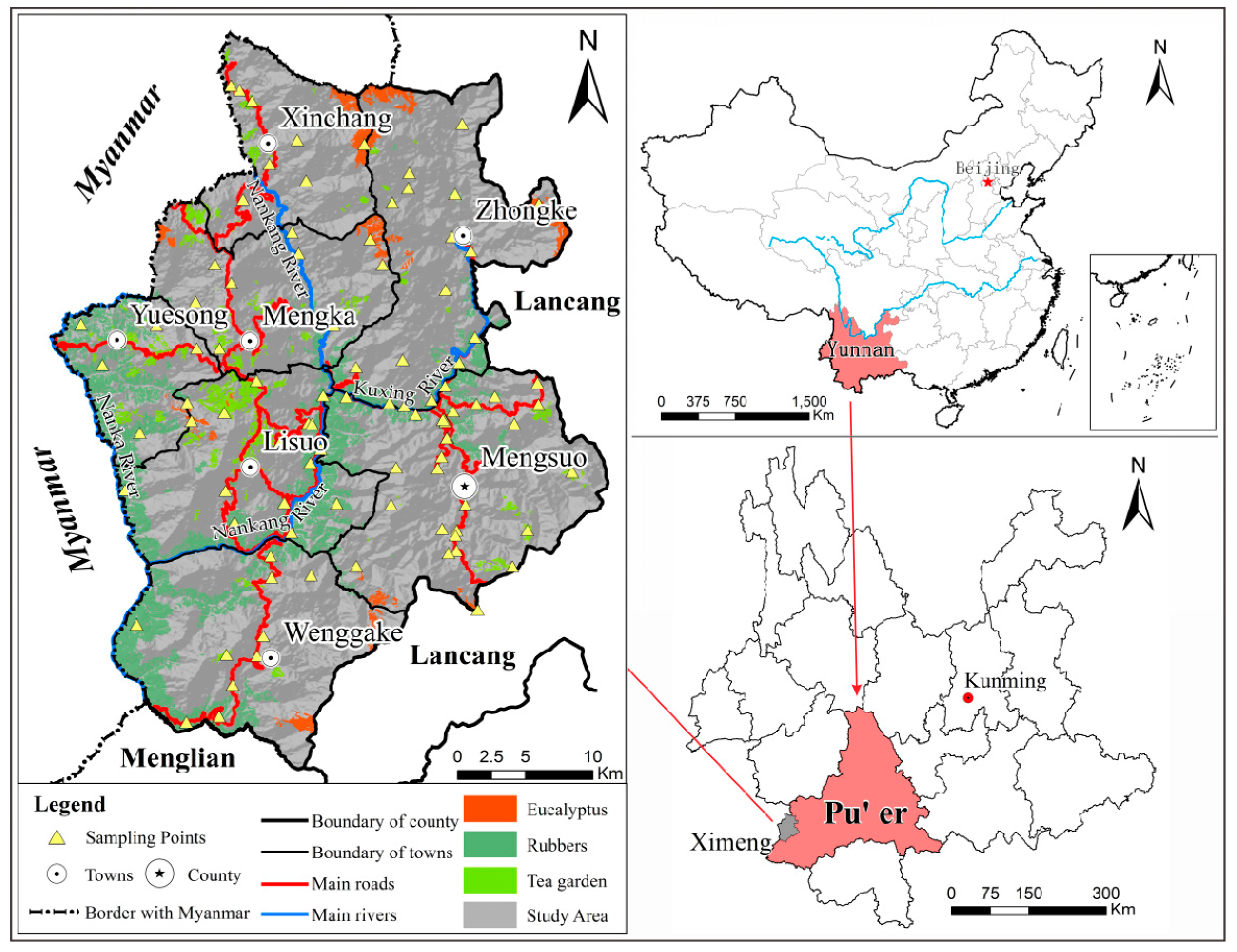
Ximeng County (99°18′–99°43′ E; 22°25′–22°57′ N) is located in the Yunnan Province, southwestern China, with 89 km of border with Myanmar; covers an area of about 1258 km² (Figure 1). The county is mountainous, ranging in elevation from 590 to 2459 m. It is influenced by subtropical oceanic monsoons. The mean annual temperature is about 15 °C; rainfall is very abundant, and the mean annual precipitation is 2758 mm. But the seasonal rainfall is uneven, with the majority being concentrated in the summer and autumn. The region is characterized by a large area of evergreen broad-leaved forests and a rich biodiversity. There are three main rivers in the county: the Nanka, Nankang, and Kuxing Rivers. Parts of the Nanka River serve as the border between China and Myanmar. The other two rivers flow from north to south into the Nanka river. In socio-economic aspects, the region is dominated by mountain agriculture; the level of economic development is relatively low, and the rural per capita annual net income was ¥ 6567 in 2015.

2.2. Data Acquisition and Processing

This study used BLRM to analyze grid-level determinants of land use change in Ximeng County. We focused on both socio-economic and natural environment factors at a 100 × 100 m grid scale. Landsat 5 TM data in 2000, 2005, 2010, and Landsat 8 OLI data in 2015, were collected from http://www.gscloud.cn/. All those data were corrected by atmospheric and geometric correction. Ten land types were extracted with classification of human-computer interaction in the ENVI 4.8 and ArcGIS 10.1 software: dry cropland, paddy field, rubber plantation, forestland, shrubs, grassland, tea garden, eucalyptus forest, construction land, and waters. Field work was done in the study area and samples of land types were collected (96 sampling points, mainly involving the land types which were difficult to distinguish and which changed a lot). The accuracies were 79.9%, 82.3% 83.4%, and 86.7% and the kappa coefficients were 0.85, 0.87, 0.91, and 0.92 in 2000, 2005, 2010, and 2015, by comparing the collected samples and the classified results.

In addition, the Land Use General Plan (2010–2020), Statistical Yearbook, precipitation data, topographic data, and soil data were collected from the Land Resources Bureau, Meteorological Bureau, Statistical Bureau of Ximeng County.

2.3. Analysis Methods

2.3.1. Analysis Methods of Land-Use Spatio-Temporal Change

Based on the study of Ma [21] and Wu [22], quantitative change characteristics of land types were used to determine the absolute variation in land-use change rates:

$$S=U_b-U_a$$

(1)

$$K=\frac{U_b-U_a}{U_a}\times 100\%$$

(2)

where S is the absolute variation in the area of a certain land type in the study period; K is the change rate of a land type; U_a and U_b is the area of a land type at the beginning and the end of the study period.

A land-use transition matrix was adopted to analyze land-use transitions quantitatively; and spatial transition rate was used to analyze the characteristics of land use change spatially:

$$S_{ij}=\left[\begin{array}{cccc}{S}_{11}& S_{12}& .& S_{1n}\\ S_{21}& S_{22}& .& S_{2n}\\ .& .& .& .\\ S_{n1}& S_{n2}& .& S_{nn}\end{array}\right]$$

(3)

$$ST=\left[\frac{{\displaystyle \sum _{i=1,j=1}^n\frac{|\Delta Sij|}{Si}}}{{\displaystyle \sum _{i=1}^{n}Si}}\right]\times 100\%$$

(4)

where S_ij is the area of the land type i converted to the land type j during the study period; ST is the spatial transition rate of land use in the study period; S_i is the area of i-th land type at the beginning of the study period; and n is the quantity of the land type. The ST is calculated in 100 × 100 m grid scale to reflect the characteristics of spatial transition.

2.3.2. Analysis Methods of Driving Factors

The study of land use change and its driving factors is very important for the adjustment of land-use structure and spatial distribution. In this regard, many scholars have relied on dynamic time series to analyze the correlation between driving factors and land use change [23]. This method solves the linear relationship between driving factors and land use change. However, in many cases, especially when the dependent variable is a categorical variable rather than a continuous one, linear regression is inapplicable, since it lacks the processing ability of spatial factors which are categorical variables. Land use change is an intricate process; it is a nonlinear relationship which affects the priority of the distribution at a specific location between the driving factors and the land-use spatial distribution [24]. In terms of computing, with or without explanatory variables, the logistic regression model can assume the probability of a set of binary results as the conditional probability by logical reasoning [25]. The β in the model reflects the influencing extent of the conditional probability with various factors (i.e., the relative importance) [26], and the OR shows the degree of correlation between them. Therefore, this study uses BLRM to deal with variable data by establishing a non-linear relationship between non-continuous data of spatial distribution of land use and continuous data of driving factors in 2000, 2005, 2010, and 2015, in order to reflect the role of driving factors on land-use spatial distribution over a period of fifteen years.

By using the BLRM, the distribution probability of a certain land type is calculated [27]. The distribution probability of land use is expressed as:

$$Pi(Y_j=1|xi)=\frac{\exp (\alpha +{\beta }_1{x}_{1,i}+{\beta }_2{x}_{2,i}+\dots +{\beta }_n{x}_{n,i})}{1+\exp (\alpha +{\beta }_1{x}_{1,i}+{\beta }_2{x}_{2,i}+\dots +{\beta }_n{x}_{n,i})}$$

(5)

$$OR=\frac{Pi}{1-Pi}$$

(6)

where P_i (Y_j = 1|x_i) is the distribution probability of a land type in a grid; β_i is the regression coefficient of the driving factor x_i and expresses the degree of influence of each factor on regional land-use distribution; OR is the ratio of occurrence probability to nonoccurrence probability; and α is the intercept.

As for the effectiveness test of logistic regression, Pontius [28] proposed that the Receiver Operating Characteristic Curve (ROC) method was a common method. The independent variables have a good interpretability on the dependent variable when the ROC value is larger than 0.7. Moreover, the percentage of correct parts is tested by the Percent Corrected Prediction (PCP) [29]. The bigger the PCP value, the closer simulated result is to reality. To compare the various factors, all the independent variables, except the categorical variables of basic farmlands preservation policy (x₈) and nature reserve policy (x₉), are standardized by z-score standardization in the software SPSS.

3. Results Analysis and Discussion

3.1. Characteristics of Land-Use Spatio-Temporal Change

3.1.1. Characteristics of Quantitative Change

The main land types in Ximeng County were forestland, dry cropland, and rubber plantations. In 2000 and 2005, the land types were mainly forestland and dry cropland. Forestland accounted for 64.15% and 57.15% of total area, whereas dry cropland accounted for 22.77% and 23.90%. In 2010 and 2015, the proportion of forestland continued to decrease to 51.03% and 48.41%, the proportion of dry cropland decreased slightly to 22.32% and 22.64%, while the proportion of rubber plantation increased significantly to 11.40% and 12.74%. In short, a large area of rubber was artificially planted, which dominated the changing pattern of the land-use structure from 2000 to 2015 (

Table 1. Land Use Quantity Change in Ximeng County.

Land Types	Area (hm2)				Absolute Variation in Area (hm2)				Change Rate of Land Use (%)
	2000	2005	2010	2015	2000–2005	2005–2010	2010–2015	2000–2015	2000–2005	2005–2010	2010–2015	2000–2015
Eucalyptus forest	657.70	2447.19	2478.53	2498.44	1789.49	31.34	19.91	1840.74	272%	1%	1%	280%
Grassland	6314.79	4693.85	4142.60	4117.98	−1620.94	−551.25	−24.62	−2196.81	−26%	−12%	−1%	−35%
Tea garden	924.03	2019.31	3410.24	3818.72	1095.28	1390.93	408.48	2894.69	119%	69%	12%	313%
Shrubs	692.91	540.83	487.56	457.10	−152.08	−53.27	−30.46	−235.81	−22%	−10%	−6%	−34%
Dry cropland	28,643.65	29,044.09	28,072.58	28,485.27	400.44	−971.51	412.69	−158.38	1%	−3%	1%	−1%
Construction land	1631.99	1857.06	1902.53	1906.07	225.07	45.47	3.54	274.08	14%	2%	0%	17%
Paddy field	5768.05	6385.24	6672.21	7332.60	617.19	286.97	660.39	1564.55	11%	4%	10%	27%
Waters	68.40	68.53	101.53	249.69	0.13	33.00	148.16	181.29	0%	48%	146%	265%
Rubber plantation	394.90	6852.30	14,339.36	16,028.52	6457.40	7487.06	1689.16	15,633.62	1635%	109%	12%	3959%
Forestland	80,701.48	71,889.5	64,190.77	60,903.53	−8811.98	−7698.73	−3287.24	−19,797.95	−11%	−11%	−5%	−25%

).

In terms of the absolute variation of land types, the areas of rubber plantation, tea garden, eucalyptus forest, paddy field, construction land, and waters showed increasing trends, while the areas of forestland, grassland and shrubs showed decreasing trend. The dry cropland changed with fluctuations. As for the change rate (K), the land types with the fastest growth rates were rubber plantations, tea gardens, eucalyptus forests, and waters in 2000–2015. The change rate of other land types was not obvious. Among them, the area cardinal number of forestland and dry cropland was too large at the beginning year, which influenced the change rate in study period (Table 1).

3.1.2. Characteristics of Spatial Change

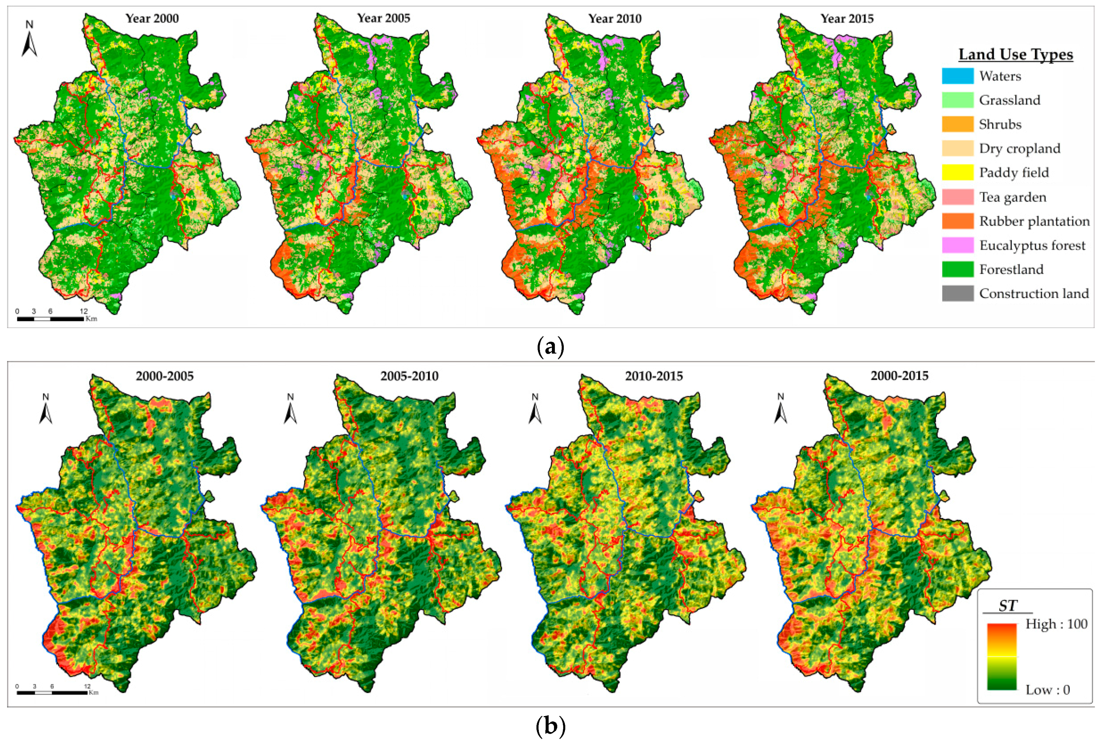
From 2000 to 2015, a large-scale planting of rubber, tea, and eucalyptus dominated the land-use transitions in Ximeng County (

Table 2. The Transition Matrix of Land Use from 2000 to 2015 (Measure Unit: hm²).

Land Types	Eucalyptus Forest	Grassland	Tea Garden	Shrubs	Dry Cropland	Construction Land	Paddy Field	Waters	Rubber Plantation	Forestland	Total in 2000
Eucalyptus forest	618.10	0.12	2.23	0.00	1.81	0.00	17.76	0.00	0.00	17.68	657.70
Grassland	87.59	2713.41	24.93	6.05	2555.28	4.33	115.75	6.96	22.68	777.80	6314.79
Tea garden	1.27	4.43	798.75	1.22	35.41	1.75	3.71	0.00	2.28	75.22	924.03
Shrubs	18.95	13.37	4.35	300.75	169.99	1.56	14.11	0.23	17.80	151.80	692.91
Dry cropland	215.51	519.34	1870.30	16.43	13,027.50	170.72	595.60	23.06	8037.43	4167.76	28,643.65
Construction land	0.01	0.86	13.82	1.54	123.59	1273.04	39.42	0.08	25.88	153.75	1631.99
Paddy field	0.36	50.00	30.40	15.33	324.56	55.75	4700.91	1.11	119.58	470.04	5768.05
Waters	0.00	0.81	0.00	0.00	2.69	0.41	0.00	59.84	0.40	4.24	68.40
Rubber plantation	0.00	0.00	0.00	3.30	1.12	0.71	1.37	0.25	346.75	41.40	394.90
Forestland	1556.65	815.64	1073.93	112.48	12,243.31	397.80	1843.97	158.15	7455.71	55,043.84	80,701.48
Total in 2015	2498.44	4117.98	3818.72	457.10	28,485.27	1906.07	7332.60	249.69	16,028.52	60,903.53	125,797.91

and Figure 2). The increased area of tea gardens (2894.69 hm²) and rubber plantation (15,633.62 hm²) were mainly converted from dry cropland and forestland. The increased area of eucalyptus forest (1840.74 hm²) was mainly converted from forestland, dry cropland, and grassland. The area of construction land increased (274.28 hm²) by mainly occupying forestland and dry cropland. The area of waters increased (181.29 hm²) because of the construction of Hydropower Stations in Nanhong River and Fumunai Reservoir in Mengxu Town which submerged forestland and dry cropland.

Meanwhile, there was also a large area of forestland and dry cropland that was converted to other land uses (Table 2 and Figure 2). The decreased area of forestland (19,797.95 hm²) was mainly converted to dry cropland and rubber, while there was 4167.76 hm² compensation from dry croplands by the “Grain for Green” policy. There were similar values of dry cropland between the area converted to other land types and that converted from other land types, making the amount of dry croplands more or less stable.

The spatial transition rate of land use is between 0 and 100 in Ximeng County (Figure 2b). The larger the value, the more obvious the land use changes. It can be seen that the regions with high spatial transition rates were similar to the planting areas of rubber, tea, and eucalyptus. Most of these artificial forests were planted along with the rivers or roads and occupied lots of farmlands and forests. The increase in rubber plantations contributed most to the spatial transition rate from 2000 to 2015 (Figure 2). Meanwhile, the spatial transition rate of land use had different characteristics at each time stage. In 2000–2005, eucalyptus was planted a lot in the northern area, and rubber was mainly planted along with the Nanka River and Nankang River in central and southwest area. At the same time, the expanding of cultivated land was also obvious on the basis of data from 2000. These changes caused a high spatial transition rate. In 2005–2010, land-use transitions mainly occurred in the central, southwest, and mid-eastern areas with the planting of rubber and tea. This resulted in the more gathered distribution of cultivated land. In 2010–2015, land-use transitions occurred in most areas of the county (yellow parts), but there were fewer areas with concentrated changes (red parts). Areas with high spatial transition rates also mainly involved changes of rubbers, tea, farmlands and forests in mid-eastern and mid-western regions. Artificial forests were mainly planted close to the border with Myanmar in the first five years, and then in other areas of the county close to the main rivers and roads. Overall, land-use spatial change mainly occurred along the Nanka, Nankang and Kuxing Rivers by the large-scale planting of artificial forests.

In summary, there were four spatio-temporal characteristics among the main land types: (1) Large-scale planting of artificial forests such as, rubber, tea and eucalyptus had largely replaced forestland and dry cropland. (2) Due to the “Grain for Green” policy and the large-scale planting of artificial forest, a large area of dry cropland was converted to forestland and rubber plantation. But at the same time, forests had been cut down and converted to dry cropland because local households were expanding farming activities to maintain their livelihoods. (3) The construction land expanded significantly by occupying forestland and dry cropland. (4) The increased water areas mainly came from forestland and dry cropland due to reservoir submerging.

3.2. Driving Factors of Land Use Change

As introduced above, driving factors of land use change were selected from both socio-economic and natural environment aspects (

Table 3. Factors determining the land-use spatio-temporal changes in Ximeng County.

Category	Subcategory	Variable	Code
Socio-economic factors	Accessibility	Distance to the main road	x1
		Distance to the rural road	x2
		Distance to the town	x3
		Distance to the rural settlement	x4
	Development of local community	Population	x5
		Rural per capita net income	x6
	Land use spatial configuration	Distance to previous land use	x7
	Political restriction	Basic farmlands preservation policy	x8
		Nature reserve policy	x9
Natural environment factors	Topography	Slope	x10
		Elevation	x11
		Aspect	x12
	Potential productivity	Soil organic matter	x13
		Soil types	x14
		Annual mean precipitation	x15
		Distance to river	x16
		Distance to irrigation canal	x17

). Variables such as technology and culture were ignored due to data unavailability. In this study, all data is processed to a regular grid scale of 100 × 100 m in the ArcGIS 10.1 (ESRI, Redlands, USA) before being added to the BLRM. Except for the x₈, x₉, and x₁₄, all other factors are continuous variables.

3.2.1. Socio-Economic Factors

Socio-economic factors, including accessibility, development of local community, land-use spatial configuration and political restriction, are selected to reflect mankind’s ability to exploit the natural environment in the study.

(1)

The accessibility of certain land areas, indicating the distance to roads, railways, ports, villages, and centers of economic activity, is frequently used as one of main socio-economic factors [30]. The accessibility of rural areas and markets is related to market expansion and the commercialization of agriculture, which can affect the profitability of land use and farmers’ willingness to land use [31]. There are many rivers and streams as irrigation sources rather than transportation in the study area. Therefore, the distance to rivers is analyzed as a natural environment factor for agriculture-related land use changes. Based on accessibility, the distance to main roads, to local rural roads, to towns, and to rural settlements are selected. The data of roads, towns, and rural settlements was adopted from “The Land Use General Plan of Ximeng County (2010–2020)”, and the Euclidean distance of those data are used to describe the accessibility.

(2)

The development of local communities, regarding population, income, labor, and technology, can also influence deforestation and the abandoning of cultivated lands, and thus, influence land-use spatial distribution. As the indexes of local community development, population and rural per capita net income are selected from Statistical Yearbook of Ximeng County in 2000, 2005, 2010, and 2015.

(3)

The expansion of land always bases on the previous land use, or presents enclave expansion, such as the spatial expansion of construction land. Land-use spatial allocation is also influenced by previous land uses and surrounding land. Therefore, the proximity to previous land use is also considered as a variable.

(4)

Policy factors are considered in many studies on land use changes [32]. The cultivated land and the ecological land in the study areas are generally restricted to changes under the protection policies of basic farmland preservation and nature reserves. Thus, they are introduced in the regression model as dummy variables.

3.2.2. Natural Environment Factors

Natural environment factors are the basic parameters for determining land-use spatio-temporal changes including topography and land potential productivity, especially for agricultural areas like the case area in this study. Generally, forestland on low elevation and gentle slope is more likely to be reclaimed for other uses, while cultivated land on high elevation and with steep slopes is more likely to be abandoned and converted to artificial forest such as rubber plantation [30]. So, elevation and slope are the main natural elements affecting the land-use spatio-temporal change. The potential productivity of land, influenced by soil properties and climate conditions, affects the land-use spatio-temporal change according to economic factors. Therefore, slope, elevation, and aspect deriving from the DEM data, soil organic matter, and soil types deriving from the soil thematic map, and annual mean precipitation deriving from the interpolation results of weather station data in each town in Ximeng County, are considered in our regression model. Depending on the physical and chemical properties of the soil and the degree of ripening, the soil types (x₈) are divided into six categories (from 6 to 1): paddy soils, yellow-brown earths, yellow earths, red earths, lateritic red earths and humid-thermo ferralitic. Moreover, since rivers play a key role in the irrigation of the study area, the distance to a river and the distance to an irrigation canal can also influence the potential productivity of land, and are also selected as natural environment factors in the model.

3.3. Driving Factors Analysis of Land-Use Spatio-Temporal Change

According to the characteristics of land-use spatio-temporal change in Ximeng County, the main land types were forestland, dry cropland, and rubber plantations. Drastic changes in the proportion of rubber plantation, tea garden, dry cropland, forestland and construction land are the major causes of the regional land-use spatio-temporal change. Thus, it is necessary to analyze the driving factors of these main land types with major changes (cultivated land consists of dry cropland and paddy fields). In the BLRM, the basic farmland preservation policy (x₈) and nature reserve policy (x₉) were re-encoded in the software SPSS 22 as categorical variables. Being located on basic farmlands was coded as 0, while being in non-basic farmlands was coded as 1; being located in nature reserves was coded as 0, while being in non-natural reserves was coded as 1.

3.3.1. Testing the BLRM

The ROC values (got by “ROC curve” processing between probability value (P) of BLRM and spatial distribution of each land type) of forestland, cultivated land, rubber plantation, tea garden, and construction land were all more than 0.7 (

Table 4. The ROC and PCP value of BLRM.

Land Uses	2000		2005		2010		2015
	ROC	PCP	ROC	PCP	ROC	PCP	ROC	PCP
Forestland	0.784	73.80%	0.813	75.40%	0.852	78.00%	0.925	85.10%
Cultivated land	0.842	79.70%	0.837	80.00%	0.804	77.60%	0.876	82.80%
Rubber plantation	0.970	99.70%	0.949	94.90%	0.952	92.10%	0.960	92.40%
Tea garden	0.915	99.30%	0.879	98.40%	0.901	97.20%	0.986	98.40%
Construction land	0.932	98.70%	0.929	98.60%	0.924	98.50%	0.979	98.90%

), indicating that the established BLRM was good for the analysis. The PCP values of cultivated land and forestland were 70% to 85%. It is effective to use BLRM to predict the change of cultivated land and forestland. The PCP values of construction land, rubber plantations, and tea gardens were all more than 90% (Table 4), meaning that the model had an ideal prediction ability for these three land types. Similarly, their standard errors (S.E.) were all less than 1.0 (

Table 5. Results of BLRM of Forestland.

Variable	2000 (ROC = 0.784)			2005 (ROC = 0.813)			2010 (ROC = 0.852)			2015 (ROC = 0.925)
	β	S.E.	OR	β	S.E.	OR	β	S.E.	OR	β	S.E.	OR
x1	0.149	0.008	1.161	−0.043	0.009	0.958	0.155	0.008	1.167	−0.037	0.008	0.964
x2	0.201	0.010	1.222	0.243	0.010	1.275	0.130	0.100	1.138	0.001	0.042	1.001
x3	0.035	0.009	1.035	−0.457	0.011	0.633	−0.079	0.009	0.924	−0.018	0.008	0.982
x4	0.535	0.010	1.708	0.600	0.010	1.821	0.562	0.010	1.753	−0.126	0.010	0.882
x5	N 1	N	N	−0.228	0.008	0.796	−0.073	0.008	0.930	−0.015	0.003	0.985
x6	−0.199	0.008	0.820	−0.271	0.009	0.763	−0.043	0.008	0.958	0.191	0.011	1.210
x8	1.375	0.014	3.956	1.857	0.016	6.407	1.601	0.014	4.959	2.257	0.032	9.553
x9	−0.624	0.083	0.536	−0.214	0.079	0.807	−0.270	0.078	0.763	−0.589	0.137	0.555
x10	0.187	0.007	1.205	0.229	0.007	1.258	0.208	0.007	1.231	0.026	0.002	1.026
x11	0.310	0.008	1.364	0.530	0.013	1.699	0.566	0.010	1.761	0.002	0.000	1.002
x12	−0.085	0.007	0.918	−0.139	0.007	0.870	−0.050	0.007	0.951	−0.001	0.000	0.999
x13	0.063	0.007	1.065	N	N	N	N	N	N	−0.017	0.002	0.983
x14	N	N	N	−0.107	0.011	0.899	N	N	N	−0.215	0.023	0.807
x15	N	N	N	−0.432	0.010	0.649	N	N	N	N	N	N
x16	N	N	N	0.433	0.011	1.542	0.093	0.011	1.097	N	N	N
x17	−0.172	0.007	0.842	−0.060	0.008	0.942	−0.151	0.008	0.860	N	N	N
Constant α	0.548	0.083	1.730	−0.757	0.080	0.469	−0.233	0.079	0.792	−0.831	0.236	0.436

¹ N means the value was eliminated because its β value was too small; indexes which eliminated all values in four years are not included in this table.

,

Table 6. Results of BLRM of Cultivated Land.

Variable	2000 (ROC = 0.842)			2005 (ROC = 0.837)			2010 (ROC = 0.804)			2015 (ROC = 0.876)
	β	S.E.	OR	β	S.E.	OR	β	S.E.	OR	β	S.E.	OR
x1	−0.167	0.009	0.846	−0.214	0.009	0.808	−0.117	0.009	0.889	0.088	0.009	1.092
x2	−0.499	0.013	0.607	−0.337	0.012	0.714	−0.238	0.011	0.788	−0.662	0.048	0.516
x3	0.059	0.010	1.061	N	N	N	−0.056	0.010	0.945	−0.108	0.009	0.898
x4	−0.552	0.012	0.576	−0.458	0.011	0.632	−0.514	0.011	0.598	−0.057	0.011	0.945
x5	0.041	0.010	1.042	0.153	0.008	1.166	0.183	0.008	1.201	0.090	0.004	1.094
x6	0.146	0.011	1.157	N 1	N	N	N	N	N	−0.204	0.013	0.815
x8	−1.995	0.016	0.136	−2.156	0.015	0.116	−1.813	0.015	0.163	−2.074	0.031	0.126
x9	0.843	0.121	2.323	0.882	0.113	2.415	0.848	0.109	2.334	1.332	0.204	3.790
x10	−0.170	0.008	0.844	−0.154	0.008	0.857	−0.187	0.008	0.829	−0.017	0.002	0.983
x11	−0.456	0.012	0.634	−0.431	0.009	0.650	−0.169	0.012	0.845	−0.001	0.074	0.999
x12	0.059	0.008	1.061	N	N	N	0.101	0.008	1.106	−0.139	0.151	0.870
x13	N	N	N	N	N	N	−0.032	0.008	0.968	N	N	N
x14	N	N	N	N	N	N	−0.038	0.011	0.962	0.256	0.021	1.292
x15	N	N	N	N	N	N	−0.127	0.009	0.880	0.200	0.090	1.221
x16	−0.120	0.012	0.887	N	N	N	N	N	N	0.073	0.062	1.076
x17	N	N	N	−0.030	0.008	0.970	−0.078	0.008	0.925	N	N	N
Constant α	−1.028	0.122	0.358	−0.815	0.114	0.443	−0.934	0.110	0.393	−0.982	0.291	0.375

¹ N means the value was eliminated because its β value was too small; indexes which eliminated all values in four years are not included in this table.

,

Table 7. Results of BLRM of Rubber Plantation.

Variable	2000 (ROC = 0.970)			2005 (ROC = 0.949)			2010 (ROC = 0.952)			2015 (ROC = 0.960)
	β	S.E.	OR	β	S.E.	OR	β	S.E.	OR	β	S.E.	OR
x1	−0.721	0.085	0.486	N 1	N	N	0.179	0.016	1.196	−0.119	0.017	0.888
x2	0.233	0.079	1.262	0.137	0.023	1.147	−0.213	0.020	0.808	−0.407	0.084	0.666
x3	N	N	N	0.748	0.018	2.114	0.910	0.018	2.485	0.154	0.014	1.166
x4	−0.508	0.102	0.602	−0.322	0.025	0.725	−0.175	0.021	0.839	0.043	0.020	1.043
x5	−1.520	0.113	0.219	−0.113	0.020	0.893	0.197	0.013	1.217	−0.044	0.006	0.957
x6	1.240	0.125	3.455	−0.211	0.038	0.810	0.347	0.014	1.415	−0.008	0.019	0.992
x8	2.805	0.309	16.528	N	N	N	−1.016	0.027	0.362	−1.445	0.051	0.236
x10	0.280	0.052	1.324	0.044	0.016	1.045	0.115	0.013	1.121	0.011	0.003	1.011
x11	−1.973	0.142	0.139	−2.579	0.045	0.076	−2.805	0.035	0.061	−0.009	0.184	0.991
x12	−0.344	0.060	0.709	−0.105	0.016	0.901	0.041	0.013	1.042	N	N	N
x13	−0.916	0.077	0.400	−0.079	0.020	0.924	0.043	0.016	1.044	0.022	0.004	1.023
x14	−1.257	0.167	0.285	−0.606	0.038	0.546	−0.224	0.028	0.799	−0.634	0.045	0.530
x15	N	N	N	N	N	N	0.999	0.027	2.716	0.002	0.173	1.002
x16	N	N	N	−0.573	0.034	0.564	−0.652	0.025	0.521	N	N	N
x17	N	N	N	0.207	0.019	1.229	0.265	0.016	1.303	0.074	0.007	1.077
Constant α	−12.598	0.382	0.000	−6.136	0.052	0.002	−4.355	0.036	0.013	3.376	0.416	29.263

¹ N means the value was eliminated because its β value was too small; indexes which eliminated all values in four years are not included in this table.

,

Table 8. Results of BLRM of Tea Garden.

Variable	2000 (ROC = 0.915)			2005 (ROC = 0.879)			2010 (ROC = 0.901)			2015 (ROC = 0.986)
	β	S.E.	OR	β	S.E.	OR	β	S.E.	OR	β	S.E.	OR
x1	−0.972	0.063	0.379	−0.373	0.033	0.689	−0.214	0.032	0.807	−0.121	0.028	0.886
x2	−0.875	0.083	0.417	−0.498	0.051	0.608	N 1	N	N	N	N	N
x3	−0.163	0.051	0.850	−0.691	0.032	0.501	−0.457	0.043	0.633	−0.114	0.021	0.893
x4	−0.410	0.054	0.664	−0.752	0.038	0.472	−3.748	0.086	0.024	−0.127	0.032	0.881
x5	−0.908	0.066	0.403	−0.265	0.027	0.767	−0.080	0.030	0.923	−0.054	0.010	0.948
x6	0.603	0.065	1.827	0.064	0.024	1.066	N	N	N	−0.180	0.027	0.835
x8	−1.460	0.074	0.232	−1.210	0.050	0.298	2.714	0.121	15.091	−1.659	0.080	0.190
x9	N	N	N	0.617	0.198	1.854	−0.569	0.189	0.566	2.117	0.597	8.309
x10	−0.294	0.041	0.745	−0.257	0.027	0.773	−0.680	0.032	0.506	−0.026	0.005	0.974
x11	0.752	0.060	2.121	0.880	0.049	2.411	N	N	N	N	N	N
x12	0.391	0.040	1.478	0.123	0.025	1.131	N	N	N	0.030	0.372	1.030
x13	−0.154	0.042	0.857	−0.111	0.026	0.895	N	N	N	0.016	0.007	1.016
x14	N	N	N	−0.165	0.038	0.848	−0.155	0.032	0.856	−0.117	0.052	0.889
x15	N	N	N	N	N	N	−0.267	0.038	0.766	N	N	N
x16	0.684	0.058	1.982	0.437	0.040	1.548	0.296	0.040	1.344	0.099	0.153	1.104
x17	0.125	0.036	1.133	−0.124	0.027	0.883	0.250	0.028	1.284	0.157	0.011	1.170
Constant α	−5.918	0.086	0.003	−5.158	0.206	0.006	−9.314	0.239	0.000	−9.707	0.772	0.000

¹ N means the value was eliminated because its β value is too small; indexes which eliminated all values in four years are not included in this table.

and

Table 9. Results of BLRM of Construction Land.

Variable	2000 (ROC = 0.932)			2005 (ROC = 0.929)			2010 (ROC = 0.924)			2015 (ROC = 0.979)
	β	S.E.	OR	β	S.E.	OR	β	S.E.	OR	β	S.E.	OR
x1	−0.220	0.035	0.803	−0.162	0.031	0.851	−0.214	0.032	0.807	−0.129	0.031	0.879
x3	−0.220	0.034	0.803	−0.302	0.032	0.739	−0.457	0.043	0.633	−0.139	0.025	0.870
x4	−4.219	0.104	0.015	−3.786	0.088	0.023	−3.748	0.086	0.024	−0.035	0.029	0.965
x5	0.113	0.030	1.120	N 1	N	N	−0.080	0.030	0.923	N	N	N
x8	2.373	0.115	10.728	2.709	0.123	15.008	2.714	0.121	15.091	2.223	0.200	9.238
x9	N	N	N	N	N	N	−0.569	0.189	0.566	−0.521	0.227	0.594
x10	−0.709	0.035	0.492	−0.710	0.033	0.492	−0.680	0.032	0.506	−0.123	0.007	0.884
x11	0.319	0.042	1.376	0.212	0.046	1.236	N	N	N	−0.493	0.206	0.611
x14	−0.244	0.040	0.783	−0.240	0.038	0.787	−0.155	0.032	0.856	0.091	0.072	1.095
x15	N	N	N	N	N	N	−0.267	0.038	0.766	−0.305	0.241	0.737
x16	N	N	N	0.131	0.042	1.139	0.296	0.040	1.344	N	N	N
x17	0.215	0.029	1.240	0.225	0.028	1.252	0.250	0.028	1.284	0.019	0.009	1.019
Constant α	−10.318	0.163	0.000	−10.004	0.156	0.000	−9.314	0.239	0.000	−2.167	0.685	0.115

¹ N means the value was eliminated because its β value is too small; indexes which eliminated all values in four years are not included in this table.

), meaning that the model was reliable.

3.3.2. Driving Factors Analysis of Main Land Types

(1) Driving factors analysis of forestland

According to results of the BLRM (Table 5), the main driving factors of spatial distribution of forestland in 2000 were basic farmlands preservation policy (x₈), nature reserve policy (x₉), distance to rural settlements (x₄) and elevation (x₁₁). The coefficient β and OR value of x₈ were the largest, i.e., 1.375 and 3.956 respectively, and the β and OR of x₉ were −0.624 and 0.536 respectively. This indicated that the forestland was mainly distributed outside the basic farmlands and inside the nature reserves. The coefficient of x₄ (β = 0.535, OR = 1.708) and x₁₁ (β = 0.310, OR = 1.364) indicated that the distribution of forestland was positively correlated with the distance to the rural settlement and elevation. In addition, the distance to a main road (x₁), distance to a rural road (x₂), distance to a town (x₃) and soil organic matter (x₁₃) had smaller influences on the spatial distribution of forestland.

In 2005 and 2010, the main driving factors were basic farmlands preservation policy (x₈), distance to the rural settlement (x₄) and elevation (x₁₁). The influence of nature reserve policy (x₉) decreased with the reduction of coefficient β. However, there was still a large influence of x₈, x₄ and x₁₁. The x₈ (β = 1.857, 1.601; OR = 6.407, 4.959), x₄ (β = 0.600, 0.562; OR = 1.821, 1.753) and x₁₁ (β = 0.530, 0.566; OR = 1.699, 1.761) showed a strong positive relationship with the distribution of forestland.

In 2015, the distribution of forestland was mainly affected by basic farmland preservation policy (x₈) and nature reserve policy (x₉). The β and OR of x₈ were the largest, i.e., 2.257 and 9.553 respectively. The β of x₉ was −0.589 and the OR was 0.555. The forestland was well protected by nature reserves, and mainly distributed outside the basic farmland areas (Table 5).

In short, the spatio-temporal change of forestland was mainly affected by the basic farmland preservation policy, nature reserve policy, distance to the rural settlement, and elevation from 2000 to 2015. Basic farmlands and natural reserves are policy factors. Basic farmlands limit the scope of high-quality arable land, and have very small probability of being transfered to other land-types. Exploitation and utilization are prohibited in nature reserves. The Mengsuo Longtan and Sanfozu County Nature Reserve, with 50.48 km² of protected forests, limits external interference. However, the impact of nature reserves is not so obvious. The distribution of forestland has positively correlated with distance to the rural settlement and elevation, which is prone to distribution in regions which are far from rural settlements. This mainly because rural settlements and high-quality arable land are usually distributed in regions which are flat and adjacent, and the areas far from rural settlements are less affected by humans. Meanwhile, low altitude areas where near rivers are planted with rubber. Forestland was distributed in the high mountains where less interference from human beings occurs.

(2) Driving factor analysis of cultivated land

From 2000 to 2015, the spatial distribution of cultivated land was mainly affected by the basic farmlands preservation policy (x₈), nature reserve policy (x₉), distance to a rural settlement (x₄) and to a rural road (x₂), although the effect of each variable was different. The absolute value of β of x₈ were the largest, with −1.995, −2.156, −1.813, and −2.074 in these four years, indicating that the basic farmlands preservation policy strongly determined the distribution of cultivated land. The β of x₉ (0.843, 0.882, 0.848, 1.332) indicated that the distribution of cultivated land was also affected by the nature reserve policy, and the influencing degree increased in 2015. According to the β of x₄ (−0.552, −0.458, −0.514, −0.057) and x₂ (−0.499, −0.337, −0.238, −0.662), the distribution of cultivated land was negatively correlated with the distance to a rural settlement and to a rural road. There were significant differences in influence of these four factors. Based on the size of β and OR, when the factors changed, the influence is: x₈ > x₉ > x₄ > x₂ (Table 6).

To summarize, the spatio-temporal changes of cultivated land were mainly determined by the policy of basic farmlands and nature reserves, and the distance to a rural settlement and to a rural road. The first two factors have the greatest influence. Liu [33] showed that urban expansion and regional economic development played a principle role in the decrease of cultivated land. But since the State Council approved “Notice on the Guidance on Basic farmlands Protection in the Country” in 1992, and issued “Regulations on the protection of basic farmland” in 1994, the delineation of basic farmland preservation areas has been carried out nationwide, implementing extremely stringent protection regulations. Policies play a decisive role in the distribution of cultivated land. Nature reserves forbid farming, and the extent of this restriction has become more and more forceful in recent years. Other social factors, such as the distance to a rural settlement and to a rural road have a strong influence on farmlands. The distribution of cultivated land is negatively correlated with them because of the effect of accessibility, tending to distribute in regions close to the residential areas and roads. Liu [34] studied the driving forces of farmland change in Nanjing, concluding that the distribution of cultivated land was related to the distance to rural settlements and roads. Spatial distance has always been the main factor affecting the behavior of farmers. The expansion of rural settlements, roads and other construction lands accelerates the change rate of cultivated land. Farmers tend to plant crops in regions which are closer to residential zones or which have good accessibility. Until 2015, the influence of distance to rural settlements reduced, and that of distance to rural roads increased. This means that the improvement of traffic conditions and rural roads provides more convenience for farming and the transportation of agricultural fertilizers and products.

(3) Driving factors analysis of rubber plantation

In 2000, the spatial distribution of rubber plantations was positively correlated with the basic farmlands preservation policy (x₈), with the highest β and OR (2.805, 16.528). Rubber plantations showed a preference for distribution outside basic farmlands (Figure 2a). According to the β of elevation (x₁₁, β = −1.973), population (x₅, β = −1.520), and soil type (x₁₄, β = −1.257), the spatial distribution of rubber showed a negative relationship with x₁₁, x₅, and x₁₄. This implies that rubber plantations tended to be distributed in low altitude areas with low population densities, with the additional requirement of good soil type.

In 2005, as in 2000, the spatial distribution of rubber plantations was negatively correlated with elevation (x₁₁, β = −2.579) and soil type (x₁₄, β = −0.606). In addition, it was negatively correlated with distance to river (x₁₆, β = −0.573), and positively correlated with distance to a town (x₃, β = 0.748). Rubber plantations tended to be distributed in regions which were close to rivers but far from towns.

In 2010, the spatial distribution of rubber plantations was negatively correlated with elevation (x₁₁, β = −2.805), the basic farmlands preservation policy (x₈, β = −1.016), and the distance to a river (x₁₆, β = −0.652). It was positively correlated with annual mean precipitation (x₁₅, β = 0.999) and the distance to a town (x₃, β = 0.910). Areas with abundant rainfall which were far from towns tended to be planted with rubber. The negative correlation with x₈ indicates that rubber plantations were distributed in areas with coding “0”, meaning that part of the rubber even occupied farmlands with large-scale planting (Figure 2a).

In 2015, the basic farmland preservation policy (x₈, β = −1.445) and soil type (x₁₄, β = −0.634) played important roles in the distribution of rubber plantations. It indicated that rubber occupied part of basic farmlands where the soil conditions were suitable (Table 7).

In short, from 2000 to 2015, there were fluctuations in the driving factors of the spatial distribution of rubber plantations. The main reason was that the planting scale of rubber plantations increased over these fifteen years. It had a small planting area in 2000; then, the scale increased dramatically in 2005 and 2010, and its extent was mitigated in 2015. Therefore, the most representative variables in 2005 and 2010 were used to explain the characteristics of the spatial distribution of rubber. These changes were mainly affected by elevation and distance to a town and to rivers. In some cases, the basic farmland preservation policy, annual rainfall, and soil types were also important driving factors. Ray [35] proved that the climate was an important factor affecting the distribution of rubber plantations. In general, humid climate conditions are conducive to the growth of rubber, and the areas with a deficit of soil water will limit its growth [36]. Areas of low elevation have a good condition with water, heat, and light, which is more appropriate to cultivating rubber. Therefore, rubber plantations will tend to be distributed in low-altitude areas that are close to the rivers and have enough precipitation and water (Figure 2a). Changes of soil type need a long time, so this may have a smaller influence than other climate factors [37]. The species distribution not only depends on the natural environment, but also on land use, cultural customs, and other social characteristics. Rubber plantations are different from cultivated land. Their management is more extensive, so they show a distribution which is similar to that of natural forest. In consideration of farmers’ behavior, the regions close to residential zones will focus more on farmlands, so rubber has to be distributed in areas with suitable transportation. But with large-scale planting, part of rubber occupies high-quality farmlands as well.

(4) Driving factors analysis of tea garden

In 2000, the factors affecting the spatial distribution of tea gardens were mainly basic farmland preservation policy (x₈, β = −1.460), distance to a main road (x₁, β = −0.972), population (x₅, β = −0.908), and distance to a rural road (x₂, β = −0.875). They all showed a negative relationship, indicating that tea gardens occupied some basic farmlands and tended to be distributed in areas near to roads and with fewer human activities. This was positively correlated with elevation (x₁₁, β = 0.752), indicating that tea gardens tended to be distributed at high altitudes.

In 2005, the factors changed somewhat. The main driving factors were the basic farmland preservation policy (x₈, β = −1.210), elevation (x₁₁, β = 0.880), distance to the rural settlements (x₄, β = −0.752), and distance to a town (x₃, β = −0.691). The spatial distribution of tea gardens was negatively correlated with these, except for elevation.

In 2010, the main driving factors were distance to a rural settlement (x₄, β = −3.748) and basic farmland preservation policy (x₈, β = 2.714). With the development of planting technology for tea gardens, the restriction of distance to a town (x₃) and elevation (x₁₁) decreased.

In 2015, the nature reserve policy (x₉) became a main factor, and showed a positive correlation with the spatial distribution of tea gardens. The distance to a rural settlement (x₄) was not the main factor, along with the development of transportation and planting technology (Table 8).

In short, as with rubber plantations, the factors affecting the spatial distribution of tea gardens were different from 2000 to 2015. It was not obvious in terms of the characteristics of spatial distribution in 2000, because of the small planting scale of tea gardens in 2000. So, the main driving factors in 2005 and 2010 were used to explain the characteristics of the spatial distribution of tea gardens. The spatio-temporal changes of tea gardens in Ximeng County were mainly affected by distances to rural settlements and the basic farmland preservation policy. The influence of elevation and distance to a town has reduced in the last two years. Domestic scholars studied the ecological sustainability of tea gardens. For example, Jin [38] took natural conditions to evaluate the ecological sustainability of tea gardens in Lincang (southwest of Pu’er city in Yunnan). He thought that elevation (1300–1800 m) and the presence of terraced slopes (below 30 degrees) yielded the most suitable areas for tea growing. Yang [39] analyzed the effect of urban centers, roads, and other social factors to discuss the distribution of tea gardens in Pu’er, and showed that natural site conditions were the decisive factors for tea planting. Nevertheless, this study suggests that although the distribution of tea gardens is strongly related to natural factors such as elevation, socio-economic factors have become the main driving factors because of the increase of planting scale in recent years. Relatively speaking, the requirements of management and maintenance of tea gardens are higher than those of rubber plantations. Tea gardens are mainly distributed in areas close to towns and rural settlements affected by the reachability of farmers’ management. And the reduced costs of tea gardens associated with the development of roads and technology in recent years. At the same time, the policy of basic farmlands and nature reserves also places strong restrictions on the distribution of tea gardens, in spite of the fact that some basic farmlands are occupied by tea gardens and the increasing market demand (Figure 2a).

(5) Driving factors analysis of construction land

In 2000, 2005, and 2010, the main driving factors of the spatial distribution of construction land were distance to a rural settlement (x₄), basic farmland preservation policy (x₈), and slope (x₁₀). Additionally, nature reserve policy (x₉) also played a key role in 2010. In BLRM, the coefficient of x₄ (β = −4.219, −3.786 and −3.748), x₈ (β = 2.373, 2.709 and 2.714), and x₁₀ (β = −0.709, −0.710 and −0.680) meant that the distribution of construction land was negatively correlated with distance to a rural settlement and slope, while being positively correlated with basic farmland preservation policy. And the size of β revealed that when these factors changed, the influence was: x₄ > x₈ > x₁₀.

In 2015, the main driving factors were the basic farmland preservation policy (x₈, β = 2.223), nature reserve policy (x₉, β = −0.521), and elevation (x₁₁, β = −0.493). The basic farmland preservation policy maintained a strong positive correlation. Nature reserve policy and elevation showed a negative correlation. The data indicated that construction land tended to be distributed in low altitude areas and was influenced by the nature reserves (Table 9).

In short, the spatio-temporal change of construction land in Ximeng County is mainly affected by the distance to a rural settlement, basic farmland preservation policy, and slope. Construction land is negatively correlated with distance to a rural settlement. On the one hand, rural settlements are a part of construction land. The expansion of construction land is based on the original urban and rural settlements, so construction land tends to be distributed in flat areas which are suitable for the construction. On the other hand, with the increase in population, the development of roads and commercial sectors, rural settlements are continuously expanding. Although the influence of basic farmlands has decreased, it is also the main limitation of the expansion of construction land. Due to the limitation of basic farmland protection policy which prohibits construction in basic farmlands, construction land tends to be distributed in areas outside basic farmlands. Yang [40] carried out a suitability assessment of construction land in mountainous regions. He thought that good conditions for construction work existed where the slope was below 8 degrees, due to the steep slope in some areas not only increasing the cost of construction, but also causing geological disasters. Due to the destruction of the environment and other consequences, slope becomes one of the important indicators for restricting the distribution of construction land. In recent years, the influence of nature reserve policy and elevation have increased. Nature reserves prohibit human activities. In 2015, the distribution of construction land was negatively correlated with elevation, which tended to be distributed in low-altitude areas. The main reason for this is that the study area is located in a mountainous area and is not suitable for the survival of mankind in a very high elevation region. Furthermore, elevation has a close relationship with slope. The places with high altitude tend to have steep slopes and are not suitable for construction.

Socio-economic factors and natural environment factors which related to the land-use spatio-temporal change in Ximeng County are selected to established the BLRM. The results of the study are same as those of Doorn [41] and Prishchepov [42], etc. In general, both natural environment and socio-economic factors are the driving factors of land use change, but socio-economic factors have a more direct influence than natural environment factors. There is a strong influence for most land types by socio-economic factors, (e.g., policy and accessibility). However, natural environment factors, (e.g., elevation and slope), only affect the spatio-temporal change of a certain land type notably in a long period. Although the change of different land types shares some main driving factors in time and space, there are quite a few differences in terms of influence.

3.4. Discussion of Research Frame and Prospect

As a whole, land-use spatio-temporal change and the approaches are very important research directions. Lee [43,44] launched an innovative series of R packages, such as CARBayes and CARBayesST, which can fit models with different spatio-temporal structures by Conditional Autoregression Priors. These can help to realize spatio-temporal modeling of land use, such as spatio-temporal structure, interaction, clustering, autoregression, and so on. Chen [45] established three scenarios and simulated the industrial structure and spatio-temporal evolution of Township and Village Enterprise (TVE) on three scales. This can help to prevent the different development problems of TVEs in Beijing. And Abercrombie [46] used the Hidden Markov Model (HMM) to distinguish real land cover change from spurious land cover change in a classification time series which showed that the HMM method provides label sequences that are more accurate. Accordingly, Chen [47] revealed that the heterogeneity of land use change is complicated due to the multi-scale effect of water-land systems, resources management, and interactions of land-use behavior and benefits. Generally speaking, the spatio-temporal variation of land use and its related contents have become an important research hotspot. Based on its complexity, multi-scale analysis, multi-method synthesis, multi-viriate comparison, and multi-drivers influence will become the main ways to study land-use spatio-temporal change in the future.

This study is also based on the frame of land-use spatio-temporal change, in combination with driving factors. Land-use spatio-temporal change was analyzed by methods of land-use change rate, land-use transition matrix, and spatial transition rates in Ximeng County from 2000 to 2015. A Binary Logistic Regression Model was used to analyze the driving factors of land use change. Then, the main driving factors were summarized by temporal panel data. This can also help to provide a good support for government decision-making. In general, the research of LUCC is an intricate system of engineering. It is a workable and explicable way using the principles of BLRM to investigate the possible effects of the factors on land use change. And based on the results, future spatio-temporal evolution could be simulated in the next study by some models, such as those discussed in above paragraphs.

4. Conclusions

(1)

The main land types were forestland, dry cropland, and rubber plantations in Ximeng County. In 2000–2015, artificial forest, such as rubber plantations, tea gardens, and eucalyptus forest, were largely planted alongside the main rivers and roads in the central, southwest, mid-western, mid-eastern, and northern areas of the county. Meanwhile, the area of natural forest and dry cropland reduced. A large area of farmlands was converted to forestland by the “Grain for Green” policy. Additionally, there was still a phenomenon of deforested-land reclamation elsewhere due to the living pressures of farmers. The expansion of construction land occupied forestland and dry cropland, and the construction such as the Second-cascade Hydropower Station in Nanhong River and Fumunai Reservoir in Mengxu Town occupied forestland and dry cropland, thereby increasing the area of waters.

(2)

The driving factors of land use change had the common characters overall, but there were multiple influences in different periods in Ximeng County. The land-use spatio-temporal change in Ximeng County was mainly affected by policy (e.g., basic farmlands and natural reserve), topography (e.g., elevation and slope), accessibility (e.g., distance to rural settlements) and potential productivity (e.g., fertility, irrigation). Among them, policy factors are mandatory for land use; the topography sometimes determines the foundation of human activities; accessibility determines the convenience of human activities; the potential productivity of land determines the output of artificial forests and cultivated land. In summary, socio-economic factors have faster, stronger, and more direct influences than natural environment factors.

(3)

A Binary Logistic Regression Model (BLRM) can analyze the driving factors of land-use spatio-temporal change by determining non-continuous variables. It can handle the regression problem of non-continuous variables by revealing the quantitative relationships between land use changes and the driving factors at each scale level from a more microscopic point of view; then, the variables and dependent variables are expressed as non-linear relationships to determine the correlation between driving factors and land-use spatial distribution in a given period.

References

- Anaafo, D. Land reforms and land rights change: A case study of land stressed groups in the Nkoranza South Municipality, Ghana. Land Use Policy 2015, 42, 538–546. [Google Scholar] [CrossRef]
- Kong, X.B.; Zhang, F.R.; Wei, Q.; Xu, Y.; Hui, J.G. Influence of land use change on soil nutrients in an intensive agricultural region of North China. Soil Tillage Res. 2006, 88, 85–94. [Google Scholar] [CrossRef]
- Zhao, J.S.; Yuan, L.; Zhang, M. A study of the system dynamics coupling model of the driving factors for multi-scale land use change. Environ. Earth Sci. 2016, 75, 529. [Google Scholar] [CrossRef]
- Williams, R.A. Mitigating biodiversity concerns in Eucalyptus plantations located in South China. J. Biosci. Med. 2017, 3, 1–8. [Google Scholar] [CrossRef]
- Zhao, X.Q.; He, C.L.; Yi, Q. Soil moisture and water conservation in Eucalyptus uraphylla spp. introduction mountain area. J. Soil Water Conserv. 2012, 26, 205–210. (In Chinese) [Google Scholar]
- Ahrends, A.; Hollingsworth, P.M.; Ziegler, A.D.; Fox, J.M.; Chen, H.F.; Su, Y.F.; Xu, J.C. Current trends of rubber plantation expansion may threaten biodiversity and livelihoods. Glob. Environ. Chang. 2015, 34, 48–58. [Google Scholar] [CrossRef]
- Vihervaara, P.; Marjokorpi, A.; Kumpula, T.; Walls, M.; Kamppien, M. Ecosystem services of fast-growing tree plantations: A case study on integrating social valuations with land-use changes in Uruguay. For. Policy Econ. 2012, 14, 58–68. [Google Scholar] [CrossRef]
- Mitsuda, Y.; Ito, S. A review of spatial-explicit factors determining spatial distribution of land use/land-use change. Landsc. Ecol. Eng. 2011, 7, 117–125. [Google Scholar] [CrossRef]
- Rosa, I.M.D.; Purves, D.; Carreiras, J.M.B.; Ewers, R.M. Modelling land cover change in the Brazilian Amazon: Temporal changes in drivers and calibration issues. Reg. Environ. Change 2015, 15, 123–137. [Google Scholar] [CrossRef] [PubMed]
- Liu, J.Y.; Zhang, Z.X.; Xu, X.L.; Kuang, W.H.; Zhou, W.C.; Zhang, S.W.; Li, R.D.; Yan, C.Z.; Yu, D.S.; Wu, S.X.; et al. Spatial patterns and driving forces of land use change in China during the early 21st century. J. Geogr. Sci. 2010, 20, 483–494. [Google Scholar] [CrossRef]
- Zhao, X.Q.; Yang, S.H.; Yi, Q.; Lin, X.B.; Tan, S.C. A study on the driving forces of land-use changes in a small watershed of the Nujiang. Trop. Geogr. 2005, 25, 215–219. (In Chinese) [Google Scholar]
- Cao, Y.G.; Bai, Z.K.; Zhou, W.; Wang, J. Forces driving changes in cultivated land and management countermeasures in the three gorges reservoir area, China. J. Mt. Sci. 2013, 10, 149–162. [Google Scholar] [CrossRef]
- Du, S.H.; Wang, Q.; Guo, L. Spatially varying relationships between land-cover change and driving factors at multiple sampling scales. J. Environ. Manag. 2014, 137, 101–110. [Google Scholar] [CrossRef] [PubMed]
- Stevenson, R.J.; White, K.D. A comparison of natural and human determinants of phytoplankton communities in the Kentucky River basin, USA. Hydrobiologia 1995, 297, 201–216. [Google Scholar] [CrossRef]
- Thorn, M.; Green, M.; Scott, D.; Marnewich, K. Characteristics and determinants of human-carnivore conflict in South African farmland. Biodivers. Conserv. 2013, 22, 1715–1730. [Google Scholar] [CrossRef]
- Su, S.L.; Zhou, X.C.; Wan, C.; Li, Y.K.; Kong, W.H. Land use changes to cash crop plantations: Crop types, multilevel determinants and policy implications. Land Use Policy 2016, 50, 379–389. [Google Scholar] [CrossRef]
- Bruno, D.; Belmar, O.; Sánchez-Fernández, D.; Velasco, J. Environmental determinants of woody and herbaceous riparian vegetation patterns in a semi-arid mediterranean basin. Hydrobiologia 2014, 730, 45–57. [Google Scholar] [CrossRef] [Green Version]
- You, W.B.; Ji, Z.R.; Wu, L.Y.; Deng, X.P.; Huang, D.H.; Chen, B.R.; Yu, J.A.; He, D.J. Modeling changes in land use patterns and ecosystem services to explore a potential solution for meeting the management needs of a heritage site at the landscape level. Ecol. Indic. 2017, 73, 68–78. [Google Scholar] [CrossRef]
- Xie, H.L. Analysis of regionally ecological land use and its influencing factors based on a logistic regression model in the Beijing-Tianjin-Hebei region, China. Resour. Sci. 2011, 33, 2063–2070. (In Chinese) [Google Scholar]
- Wu, W.; Zhou, S.; Wei, Y.; Chang, T. Modeling spatial determinants of land urbanization in urban fringe. Trans. Chin. Soc. Agric. Eng. 2013, 29, 220–228. (In Chinese) [Google Scholar]
- Ma, S.Z.; Shi, M.C.; Yang, G.S.; Xu, X.T.; Yin, J. Analysis on spatiotemporal change of land use based on GIS technology: Taking Xinjiang Tarim basin as an example. Res. Soil Water Conserv. 2013, 20, 177–181. (In Chinese) [Google Scholar]
- Wu, X.; Shen, Z.Y.; Liu, R.M. Study on the regional differentiation of land use/land cover change in the upper reaches of Yangtze River. J. Basic Sci. Eng. 2008, 16, 819–829. (In Chinese) [Google Scholar]
- Wang, J.; Chen, Y.Q.; Shao, X.M.; Zhang, Y.Y.; Cao, Y.G. Land-use changes and policy dimension driving forces in China: Present, trend and future. Land Use Policy 2012, 29, 737–749. [Google Scholar] [CrossRef]
- Cui, L.J.; Gao, C.J.; Zhou, D.M.; Mu, L. Quantitative analysis of the driving forces causing declines in marsh wetland landscapes in the Honghe region, northeast China, from 1975 to 2006. Environ. Earth Sci. 2014, 71, 1357–1367. [Google Scholar] [CrossRef]
- Bonney, G.E. Logistic regression for dependent binary observations. Biometrics 1988, 43, 951–973. [Google Scholar] [CrossRef]
- Bui, D.T.; Löfman, O.; Revhaug, I.; Dick, B. Landslide susceptibility analysis in the Hoa Binh province of Vietnam using statistical index and logistic regression. Nat. Hazards 2011, 59, 1413–1444. [Google Scholar] [CrossRef]
- Li, Q.; Ren, Z.Y. Spacial statistics and simulation of the land use change based on binary logistic regression. Stat. Inf. Forum 2012, 27, 98–103. (In Chinese) [Google Scholar]
- Pontius, R.G.; Schneider, L.C. Land-cover change model validation by an ROC method for the Ipswich watershed, Massachusetts, USA. Agric. Ecosyst. Environ. 2001, 85, 239–248. [Google Scholar] [CrossRef]
- Zhang, Y.M.; Zhao, S.D.; Verburg, P.H. CLUE-S and its application for simulating temporal and spatial change of land use in Naiman Banner. J. Nat. Resour. 2003, 18, 310–318. (In Chinese) [Google Scholar]
- Echeverria, C.; Coomes, D.; Hall, M.H.P.; Newton, A.C. Spatially explicit models to analyze forest loss and fragmentation between 1976 and 2020 in southern Chile. Ecol. Model. 2008, 212, 439–449. [Google Scholar] [CrossRef]
- Büttner, B.; Kinigadner, J.; Ji, C.Y.; Wright, B.; Wulfhorst, G. The TUM accessibility atlas: Visualizing spatial and socioeconomic disparities in accessibility to support regional land-use and transport planning. Netw. Spat. Econ. 2018, 18, 385–414. [Google Scholar] [CrossRef]
- Hargrave, J.; Kis-Katos, K. Economic causes of deforestation in the Brazilian Amazon: A panel data analysis for 2000s. Environ. Resour. Econ. 2013, 54, 471–494. [Google Scholar] [CrossRef]
- Liu, X.H.; Wang, J.F.; Liu, J.Y.; Liu, M.L.; Bin, M. Quantitative analysis approaches to the driving forces of cultivated land changes on a national scale. Trans. Chin. Soc. Agric. Eng. 2005, 21, 56–60. (In Chinese) [Google Scholar]
- Liu, K.; Li, Y.E.; Wu, Q.; Shen, J.F. Driving force analysis of land use change in the developed area based on Probit regression model: A case study of Nanjing City, China. Chin. J. Appl. Ecol. 2015, 26, 2131–2138. (In Chinese) [Google Scholar]
- Ray, D.; Behera, M.D.; Jacob, J. Predicting the distribution of rubber trees (Hevea brasiliensis) through ecological niche modelling with climate, soil, topography and socioeconomic factors. Ecol. Res. 2016, 31, 75–91. [Google Scholar] [CrossRef]
- Raj, S.; Das, G.; Pothen, J.; Dey, S.K. Relationship between latex yield of Hevea brasiliensis and antecedent environmental parameters. Int. J. Biometeorol. 2005, 49, 189–196. [Google Scholar] [CrossRef] [PubMed]
- Li, B.; Zhang, F.; Zhang, L.W.; Gupta, D.K. Comprehensive suitability evaluation of tea crops using GIS and a modified land ecological suitability evaluation model. Pedosphere 2012, 22, 122–130. [Google Scholar] [CrossRef]
- Jin, Y.X. Linxiang District and Shuangjiang County Tea Garden Information Extracted Based on Remote Sense and Ecological Suitability Evaluation. Master’s Thesis, Yunnan University, Kunming, China, 2015. (In Chinese). [Google Scholar]
- Yang, Y.; He, C.Y.; Li, X.B. Evaluation of the suitability of large scale plantations of cultivated Pu’er tea in Yunnan Province based on GIS. J. Beijing For. Univ. 2010, 32, 33–40. (In Chinese) [Google Scholar]
- Yang, Z.S. Analysis on the special factors for evaluating mountainous urban construction land suitability in Yunnan Province. Res. Soil Water Conserv. 2015, 22, 269–275. (In Chinese) [Google Scholar]
- Doorn, A.M.; Bakker, M.M. The destination of arable land in a marginal agricultural landscape in South Portugal: An exploration of land use change determinants. Landsc. Ecol. 2007, 22, 1073–1087. [Google Scholar] [CrossRef]
- Prishchepov, A.V.; Müller, D.; Dubinin, M.; Baumann, M.; Radeloff, V.C. Determinants of agricultural land abandonment in post-Soviet European Russia. Land Use Policy 2013, 30, 873–884. [Google Scholar] [CrossRef] [Green Version]
- Lee, D.; Rushworth, A.; Napier, G. Spatio-temporal areal unit modeling in R with conditional autoregressive priors using the CARBayesST package. J. Stat. Softw. 2018, 84, 1–39. [Google Scholar] [CrossRef]
- Lee, D. CARBayes: An R package for Bayesian spatial modelling with conditional autoregressive priors. J. Stat. Softw. 2013, 55, 1–24. [Google Scholar] [CrossRef]
- Chen, Y.; Song, Z.J.; Zhang, G.F.; Majeed, M.T.; Li, Y. Spatio-temporal evolutionary analysis of the township enterprises of Beijing suburbs using computational intelligence assisted design framework. Palgrave Commun. 2018, 4, 31. [Google Scholar] [CrossRef]
- Abercrombie, S.P.; Friedl, M.A. Improving the consistency of multitemporal land cover maps using a Hidden Markov Model. IEEE Trans. Geosci. Remote Sens. 2016, 54, 703–713. [Google Scholar] [CrossRef]
- Chen, J.X.; Xia, J.; Zhao, Z.F.; Hong, S.; Liu, H.; Zhao, F. Using the RESC model and diversity indexes to assess the cross-scale water resource vulnerability and spatial heterogeneity in the Huai River Basin, China. Water 2016, 8, 431. [Google Scholar] [CrossRef]
Figure 1.
The Location of Ximeng County in Yunnan Province of Southwest China (land use in 2015).
Figure 2.
Land use/land cover change in Ximeng County: (a) Land-use distribution; (b) Spatial transition rate (ST) of land use in four periods.