A Practical Comparison of Regionalized Land Use and Biodiversity Life Cycle Impact Assessment Models Using Livestock Production as a Case Study

Abstract

Land use is increasingly important for impact assessment in life cycle assessment (LCA). Its impacts on biodiversity and provision of ecosystem services are crucial to depict the environmental performance of products. Life cycle impact assessment (LCIA) models are commonly selected by consensus through processes frequently misinformed by the absence of practical application studies. Here, we performed an assessment of all free and peer-reviewed LCIA models for land use. We started with spatial correlation analysis at the country scale. Models that use the same indicators are strongly correlated, suggesting that regionalization is no longer a decisive issue in model selection. We applied these models in a case study for cattle production where feeds are replaced by sown biodiverse pastures (SBP). We tested (1) a non-regionalized inventory from an LCA database and, (2) a regionalized inventory that explicit considered the locations of land occupation and transformation. We found the same qualitative result: the installation of SBP avoids impacts due to feed substitution. Each hectare of SBP installed avoids the occupation of 0.5 hectares per year for feed ingredient production. Adding inventory regionalization for 70% of land use flows leads to a change of 15% in results, suggesting limited spatial differentiation between country-level characterization factors.

1. Introduction

Life cycle assessment (LCA) is a popular method for integrated assessments of environmental impacts throughout product supply chains [1]. LCA has been used in numerous agri-food studies, in order to identify environmental hotspots and pinpoint solutions to mitigate environmental burdens [2,3,4,5,6,7]. It is often applied, in particular, to meat production, given the high indirect environmental impacts mostly related to animal feed [8,9]. Concentrate production, in particular, leads to indirect land transformations during the production of ingredients [8,10,11]. A careful analysis of livestock feed, however, is likely to show different results depending on the pasture system and region of implementation. The impacts of land use for grazing or for agricultural production of feeds, including ecosystem services generated and impacts on biodiversity, are critical for a full picture of the sustainability of meat production.

Life cycle impact assessment (LCIA) has increasingly been done with regionalized models. This trend is particularly visible given the high number of regionalized models published for land use in the past 10 years [12,13]. Prior to this, it was common to use one globally applicable characterization factor (CF) to depict the contribution of each land occupation and transformation flow in the inventory to an impact category. Spatialized models are now the norm in cases where the environmental damage has a spatial dimension [14]. These spatial models are essential to fully depict the environmental performance in areas of protection insufficiently covered by other impact categories. They are especially suited for products deeply rooted in land use processes, namely those where the agricultural stage is particularly important.

Now a new challenge has surfaced due to the availability of different models, each with their modelling approaches and data, depicting different aspects of the complex pathways involved in land use impacts—in particular, those targeting the effects on ecosystem services, soil organic carbon (SOC) depletion and biodiversity. The problem is how to address the disparities in methodologies and types of indicators used. To reference some important models that provide CFs to practitioners, thus highlighting the recent proliferation of models, Brandão and Milà i Canals [15], Alvarenga et al. [16,17], Taelman et al. [18], Morais et al. [19] and Teixeira et al. [20] all present characterization models depicting impacts from land use on biotic production (BPP). Other models, such as Saad et al. [21] and LANd use indicator value Calculation (LANCA) [22], cover related impact pathways for other types of ecosystem damage and services (including biotic production), such as erosion resistance, water purification and climatic regulation. For biodiversity impacts from land use, de Baan et al. [23], Chaudhary et al. [24] and Chaudhary and Brooks [25] are some notable examples.

Practitioners thus need guidance on how to combine these models or about which one they should choose. It has been shown that methodological choices such as the reference state can deeply influence LCIA results even for a single model [26]. Usually the approach chosen to provide guidance to practitioners is through the implementation of consensus-building initiatives led by an authoritative institution or conglomerate of institutions. This exercise typically includes the direct comparison between modelling choices, assumptions, results and institutional support for each model. The recommendation is legitimized by the process itself and by the driving institutions, which lend their credibility and expertise to the assessment, typically involving internationally recognized experts. The European Commission has led such processes during the selection of LCIA indicators that integrate the International Reference Life Cycle Data System (ILCD) guidelines [27]. The United Nations Environment Programme (UNEP)/Society of Environmental Toxicology and Chemistry (SETAC) Life Cycle Initiative is another example of a platform promoting life cycle thinking. Its Phase III activities (2012–2017) targeted consensus-building on indicators/models in LCIA for impact categories previously prioritized as highly relevant and with sufficient maturity for selection of a model [28,29], such as of land use impacts on biodiversity [30]. The Initiative performed a thorough review of biodiversity assessment of ecological models within the field of LCA and outside, and recommended one method [31]. It has an active group working on soil quality models at the time of writing.

Nevertheless, these initiatives often make decisions on the basis of incomplete information due to the lack of studies that compare LCIA models in practical applications. Small differences in assumptions or data sources can result in significantly different numerical characterization factors. Even if two models are very distinct, the regional distribution and relative difference of characterization factors may be similar. Despite the critical importance of methodological choices, indicators and data used (among others), when CFs are applied to compare impacts from products or services there is (to our knowledge) no thorough quantification of the influence those variables have on actual LCA results.

Here, we present a practical application study of LCIA models without any ex ante judgment of model assumptions and data or institutional support. We looked directly at the CFs and at the ex post results of their application in a case study. Our goal was to provide a quantification of the level of spatial agreement of comparable models, and also to quantify, in a particular case study, the differences in impact assessment results as a function of modelling choices. First, we assessed how CFs for land use and biodiversity are related, using Spearman’s ρ. We thus assess whether there is redundancy or complementarity between models. This approach can inform practitioners whether there are substantial differences between models in terms of relative biogeographical differences; if there are, a multi-indicator study is probably needed; if no significant differences can be found, it would probably be safe to select only one of the highly correlated models. Second, we applied the different methods in a case study, namely the replacement of commercial feed with high-yield sown biodiverse permanent pastures (SBP) [32]. We used this case study to also assess the influence of using regionalized inventory flows in the application of country-specific CFs. This study is aimed at assisting future consensus-building initiatives or other procedures to select regionalized LCIA models.

2. Materials and Methods

2.1. Selection of Life Cycle Impact Assessment Models

We surveyed the recent literature (2007–2018) for regionalized land use and biodiversity assessment models to apply in this study. We searched for the keywords “life cycle impact assessment”, “life cycle assessment” and “land use” using Google Scholar, and assessed the documentation for the ILCD model recommendations [27] as well as the results from UNEP/SETAC task forces on land use and biodiversity [28,29,30,31]. Then, we selected models based on the following criteria: (a) only models that provide the CFs freely were considered, e.g., in reports or supporting information of papers; and (b) models were excluded if they did not provide CFs applicable at global or at least large regional scales (e.g., European Union). We ended up with: (a) three ecosystem services models, namely, Saad et al. [21], Müller-Wenk and Brandão [33] and LANCA v2.3 [22]; (b) six land use models, namely Brandão and Milà i Canals [15], Alvarenga et al. [16,17], Taelman et al. [18], Morais et al. [19] and Teixeira et al. [20]; and (c) three biodiversity models, namely de Baan et al. [23], Chaudhary et al. [24] and Chaudhary and Brooks [25]. These models are briefly described next. Note that there are some notable exclusions from this list that should be addressed. We excluded Souza et al. [34] because it only provides CFs for some scattered countries. We also excluded Cao et al. [35] because it uses Saad et al. [21] and Müller-Wenk and Brandão [33] at the midpoint.

Saad et al. [21] provides occupation and transformation CFs for erosion resistance potential (ERP), mechanical and physicochemical water purification potentials (WPP-MF and WPP-PCF) and groundwater recharge potential (FWRP). The CFs cover seven land use classes (forest, shrubland, grassland, pasture/meadow, permanent and annual crops, urban and urban green areas). CFs are aggregated by country. This method was complemented with climate regulation potential (CRP) by Müller-Wenk and Brandão [33], referring to the soil’s capacity to uptake carbon from the air.

LANCA [22] provides CFs for BPP, ERP, WPP-MF, WPP-PCF and FWRP. We were only capable of finding CFs for occupation, covering 75 ecoinvent [36] occupation fluxes and four main classes (arable, pastures/grassland, forest and urban) under different management practices. CFs are provided by country.

Brandão and Milà i Canals [15] is an adaptation from Milà i Canals et al. [37], which is the model recommended by the ILCD handbook [38] for land use but has no scope for regionalization (i.e., one single global CF per land class). This model uses SOC as an indicator of soil quality. SOC is a proxy indicator for the biotic production capacity of the soil. This model provides CFs for occupation and transformation flows, covering nine land uses classes (long-term cultivated, full tillage, reduced tillage, no tillage, permanent grassland, paddy rice, perennial/tree crop, set-aside (<20 years) and sealed land). CFs are aggregated by climate region.

Morais et al. [19] used the same model and indicator proposed by Brandão and Milà i Canals [15] and a large number of field measurements for the European Union (more than 19,000) from the LUCASOIL database [39]. The model provides CFs for nine land uses classes (evergreen/deciduous needleleaf trees, evergreen broadleaf trees, deciduous broadleaf trees, mixed/other trees, shrubs, herbaceous vegetation, cultivated and managed vegetation, regularly flooded vegetation and urban/built-up). CFs are aggregated by climate region, ecoregion and nomenclature of territorial units for statistics (NUTS) II region, and also by country.

Teixeira et al. [20] extends the work on SOC-based CFs, using a global SOC database and several different assumptions to deal with the estimation of SOC regeneration after transformation and the general model of Koellner et al. [40]. They also proposed the first consolidation approach for land use SOC-based models (Milà i Canals [37], Brandão and Milà i Canals [15] and Morais et al. [19]). Using this approach, rather than selecting a model, they used a weighted average of CFs at similar scales to arrive at a unique consolidated CF. CFs were obtained for occupation and transformation flows, covering four land uses classes (agriculture, forest, pasture and urban). CFs are aggregated by the combination between climate region and soil type, and by country.

Alvarenga et al. [17] uses chemical exergy value loss as an indicator, based on net primary production (NPP). This method only provides CFs for one “aggregated” representative land use, at country level.

Alvarenga et al. [16] uses human appropriation of net primary production (HANPP) as an indicator. HANPP is the portion of NPP that is not available for nature, due to human use. This model provides CFs for five land use classes (forest areas, wilderness and areas with no land use, infrastructure area, pasture land and cropland), where “cropland” is divided into ten specific crops. This model provides only occupation CFs aggregated by country.

Taelman et al. [18] provide country-level CFs using NPP. The model has seven main land use classes (forest, agriculture, shrub, grassland, urban, wetland and bare areas), where each class is divided according to the state; e.g., the forest class is divided into: protected, virgin, with agricultural activities and with moderate or higher livestock density. This model provides only occupation CFs aggregated by country.

De Baan et al. [23] used the total potential damage to biodiversity caused by land use, using as indicators potential global extinction of endemic species (mammals, birds, plants, amphibious, reptiles and the aggregated total for all taxonomic groups). This model provides occupation and transformation CFs for four land use classes (managed forest, agriculture, pasture, urban areas) for each taxonomic group. CFs are aggregated by ecoregion.

Chaudhary et al. [24] uses regional and global species loss due to land occupation and transformation (mammals, birds, amphibious, reptiles and aggregated), using the countryside species−area relationship model [41]. The model provides occupation and transformation CFs covering six land use classes (intensive forestry, extensive forestry, annual crops, permanent crops, pasture and urban) for each taxonomic group. CFs are provided aggregated by ecoregion and also by country.

Chaudhary and Brooks [25] improved the model proposed by Chaudhary et al. [24]. The most relevant innovation in this model was the introduction of land use intensity (divided into low, medium and high) for all land classes in the original paper. The model provides occupation and transformation CFs for five land classes (forest, plantation, pasture, cropland and urban) for each taxonomic group. CFs are aggregated by ecoregion and also by country.

To harmonize the models, we needed to make several transformations. First, models are frequently at different scales. As the most common unit of analysis is the country, we converted CFs from models at other scales into country-level CFs as area-weighted averages using country contours. For example, if one country is divided into two ecoregions, and only ecoregion-level CFs are available for that model, the CF for that country would be the average of the CFs for the two ecoregions weighted by the area of each. This analysis was performed using the ArcGIS 10.5 software. Second, the land classes used in the models do not match. Brandão and Milà i Canals [15] and Alvarenga et al. [16] do not provide CFs for the “forest” land use class, while Morais et al. [19] suggests that the “forest” class is an average of evergreen/deciduous needleleaf trees, evergreen broadleaf trees, deciduous broadleaf trees and mixed/other trees classes. For Taelman et al. [18] we aggregated the CFs using an average of the states of each of the main seven land use classes, to allow comparability with the other models. For LANCA [22], we aggregated land use types in “high land use intensity” for the land uses explicitly called “intensive” (e.g., “arable, intensity”), and “low land use intensity” otherwise. In all other cases we used the original classes from studies. In some cases, we made assumptions regarding the nomenclature of classes. We assumed that the “herbaceous vegetation” land use class in Morais et al. [19] was equivalent to the broad “pasture” class in other studies.

2.2. Correlation Analysis

To perform the correlation analysis between LCIA models, we used Spearman’s ρ [42]. Spearman’s ρ is a nonparametric measure of statistical dependence between two variables, as long as it can be described using a monotonic function. Correlations range between +1 and −1, where 1 is total positive correlation, 0 is no correlation, and −1 is total negative correlation. This method does not make any presuppositions about the distribution of the variables (appropriate when variables are measured on a scale that is at least ordinal or when there is no assurance of normal distribution). Correlations are performed at country scale to match the geospatial scale of current inventories and also because it is the most common unit of analysis of the models.

2.3. Case Study Application

SBP is a high-yield pasture system that maximizes production through the “biodiversity effect” on productivity (selection of productive and locally adapted grass and legume species) when subjected to correct management (involving phosphate fertilization and pH correction using limestone) [32,43,44,45,46,47]. SBP was developed in Portugal to increase yield and provide better quality feed for livestock but have also more recently been shown to sequester large amounts of carbon in soils, thus contributing to climate change mitigation [32,43,48]. Higher yield also means higher sustainable stocking rates and decreased need for feed supplementation, or even the elimination of feed supplementation during most of the year, especially when compared with the most common alternative land use system observed in farms before sowing—that is, semi-natural pastures (SNP). Reduction in feed supplementation compensates costs with SBP management. The system possesses several ecological and economic benefits [45,47,49]. Currently it is mostly located in Portugal’s “Montado” agri-forestry regions [43], which are areas of high interest for biodiversity protection [50]. However, despite their role as carbon sinks, [47,51], their effects on biodiversity have only been superficially addressed. There is some evidence that, at the plot level, biodiversity is not reduced when converting from SNP to SBP despite higher animal pressure on ecosystems due to increased stocking rates [43]. Indirect effects on biodiversity due to these conversions to SBP, as well as their indirect effects on other ecosystem services, remain to be duly and fully quantified, making this a prime case study for the application of the CFs.

2.3.1. Description of the Production Systems

Here, we used all LCIA models mentioned above to quantify the indirect impacts from land use due to the installation and maintenance of SBP. We compared two distinguished production systems. In the baseline system, cattle are fed with low-yield SNP that require feed supplementation (i.e., concentrate plus silage). This baseline was then changed into a second system where the concentrate is progressively substituted by installing high-yield SBP. There is ample empirical evidence that the first system is the baseline for the installation of most SBP in Portugal. We used a cradle-to-gate approach, considering all the impacts throughout the life cycle (off-farm impacts from raw materials to the production feed system, and on-farm emissions due to management practices in pastures) following ISO 14040 guidelines [52]. We used a comparative LCA (CLCA) approach proposed by Teixeira [47] and fully described by Morais et al. [51]. Under this approach, all flows that are common to both systems were removed from the analysis (e.g., for greenhouse gas emissions, animal emissions were excluded as no change in total stocking rate in the farm was assumed). The resulting life cycle is thus simpler and easier to interpret, as it only includes flows due to processes that are different between the two systems.

To compare the two systems, Morais et al. [51] defined as the functional unit (FU) 1 ha-equivalent of SBP per year. The “equivalent” is due to the calculation of SBP area in the final situation as a function of the amount and nutritional quality of the feed in the baseline situation (the area of SBP required is the area needed to provide feed of equal nutritional quality to the feed used in the SNP scenario). Four nutritional indicators were used to establish the nutritional equivalence between feed and SBP: crude protein (CP; estimated nitrogen content of feed), crude fiber (CF; indigestible carbohydrate component), neutral detergent fiber (NDF; measures the structural components in plant cells), and gross energy (GE; energy released by burning feed in excess oxygen).

The three necessary balance conditions are: (1) no change in total area (in the baseline situation all area is SNP, in the second situation the same area is divided into SBP and SNP); (2) nutritional equivalence between scenarios (i.e., nutritional requirements do not change with the transition to the second situation); and (3) no change in stocking rate (despite SBP being more productive than SNP). The difference in impact between scenarios in the first year, when pasture is not ready to be used as feed to build the seed bank for automatic re-sowing the following year, is:

$$\frac{{\left\{\mathrm{I}\right\}}_{\mathrm{f}}^{\mathrm{total}}-{\left\{\mathrm{I}\right\}}_{\mathrm{i}}^{\mathrm{total}}}{{\mathrm{A}}_{\mathrm{f}}^{\mathrm{SBP}}}={\left\{\mathrm{I}\right\}}^{\mathrm{SBP}}-{\left\{\mathrm{I}\right\}}^{\mathrm{SNP}}$$

(1)

and the impact differential after the first year, which depends on the nutritional equivalence between SBP and commercial feed, is:

$$\frac{{\left\{\mathrm{I}\right\}}_{\mathrm{f}}^{\mathrm{total}}-{\left\{\mathrm{I}\right\}}_{\mathrm{i}}^{\mathrm{total}}}{{\mathrm{A}}_{\mathrm{f}}^{\mathrm{SBP}}}={\left\{\mathrm{I}\right\}}^{\mathrm{SBP}}-{\left\{\mathrm{I}\right\}}^{\mathrm{SNP}}-\left(\frac{\mathsf{\epsilon }-1}{\mathsf{\epsilon }}\right)\frac{{\left\{\mathrm{NFU}\right\}}^{\mathrm{SBP}}}{{\langle \mathrm{NFU}\rangle }^{\mathrm{feed}}}{\langle \mathrm{I}\rangle }^{\mathrm{feed}}$$

(2)

where {I}_f^total is the environmental impact in the final scenario, {I}_i^total is the environmental impact in the initial scenario, {I}^SBP is the environmental impact per hectare of SBP, {I}^SNP is the environmental impact per hectare of SNP, A_f^SBP is the area of SBP installed, ε is the ratio between the nutritional forage units (NFU) of one hectare of SBP and one hectare of SNP, {NFU}^SBP are the NFU of SBP per unit of area, 〈NFU〉^feed is the NFU of commercial feed per unit of mass, and 〈I〉^feed is the environmental impact of commercial feed. “Environmental impacts”, in this case, are the sum of occupation and transformation flows from each inventory process involved in the product systems.

2.3.2. Inventory Analysis

Activity data for the pasture systems and inventory data were obtained from Morais et al. [51]. We used regionalized data for the Alentejo region for the management practices in SNP and SBP installation and maintenance [53]. SBP installation requires four operations (sowing, liming, harrowing, rolling and fertilizing), and materials (lime and phosphorus fertilizer, namely superphosphate). After installation, SBP require one superphosphate application every two years (i.e., in the years 3, 5, 7 and 9) and lime application every four years (in years 4 and 8) (Terraprima personal communication). The inventory flows for these materials, and also for the seed mixture composition of grasses and legumes, were collected from the ecoinvent v3.4 database [54].

We used two commercial feed formulations from Costa et al. [55] and also used in Morais et al. [51]. The first feed has high silage content (HF: 70% of maize silage and 30% of concentrate) and the second low silage content (LF: 30% of maize silage and 70% of concentrated feed). Inventory flows for feed ingredients were also obtained from ecoinvent [54]. In this study, the inventories for the main ingredients of the feed (maize silage and grain, wheat and barley) were regionalized for Portugal using the approach of Morais et al. [56], which is based on a regionalized adaptation of inventory guidelines produced by the Agribalyse [57] and the World Food LCA Database [58]. The inventory flows adapted for Portugal were the yield, land use, land transformation, fertilizer and pesticide use.

The inventory flows extracted for each process (material, energy and operations mentioned previously) were land occupation (m²·year) and transformation (m²). We noticed that most of the ecoinvent v3.4 processes are not regionalized at the country level. They are often representative of larger regions, e.g., Europe, or even applicable globally. We therefore followed two distinct approaches: (1) we considered that the inventory flows took place in the generic region of the inventory process where they are included, and (2) we changed the region of the first-tier inventory flows to the countries where the respective processes actually take place (

Table 1. Origin of feed ingredients and sown biodiverse permanent pasture seeds from ecoinvent [36] and from the Portuguese Association of Producers of Commercial Feeds for Animals [59].

Ingredient	Ecoinvent Origin	Regionalized Origin
Maize silage	Rest of the world	Ukraine
Maize grain	Rest of the world	Ukraine
Wheat grain	Rest of the world	Spain
Barley grain	Rest of the world	Spain
Soybean meal	Brazil	Brazil
Sunflower meal	Europe	Romania
Hydrogenated fat	Europe	Europe
Calcium carbonate	Europe	Europe
Sodium bicarbonate	Europe	Europe
Calcium phosphate	Europe	Europe
Salt	Europe	Europe
Vitamin mineral	Not considered	Not considered
SBP seeds	Rest of the world	Australia

). This process was carried out only for feed ingredients and SBP seeds. Regarding the feed, we used the data from the Portuguese Association of Producers of Commercial Feeds for Animals (in Portuguese, “Associação Portuguesa dos Industriais de Alimentos Compostos Para Animais (IACA)”) [59] that has data for the origin of ingredients. We assumed a single origin for each ingredient, which is the main exporting country for feeds used in Portugal. Regarding SBP seeds, we assumed that the seeds were produced in Australia (Terraprima personal communication). We assessed how this procedure of regionalization of part of the first tier of the inventory affects indirect land occupation and transformation in the overall comparison of the two systems for each of the characterization models.

2.2.3. Life Cycle Impact Assessment

We used all the previously presented methods in the LCIA of the case study plus an analysis of direct occupation and transformation of land by adding all inventory flows in their original units. We also used Milà i Canals [37], which is the model recommended by the International Reference Life Cycle Data System (ILCD) [38] despite the fact that this model is not regionalized (i.e., CFs without spatial differentiation). The goal was to have a benchmark for comparison with regionalized CFs.

3. Results

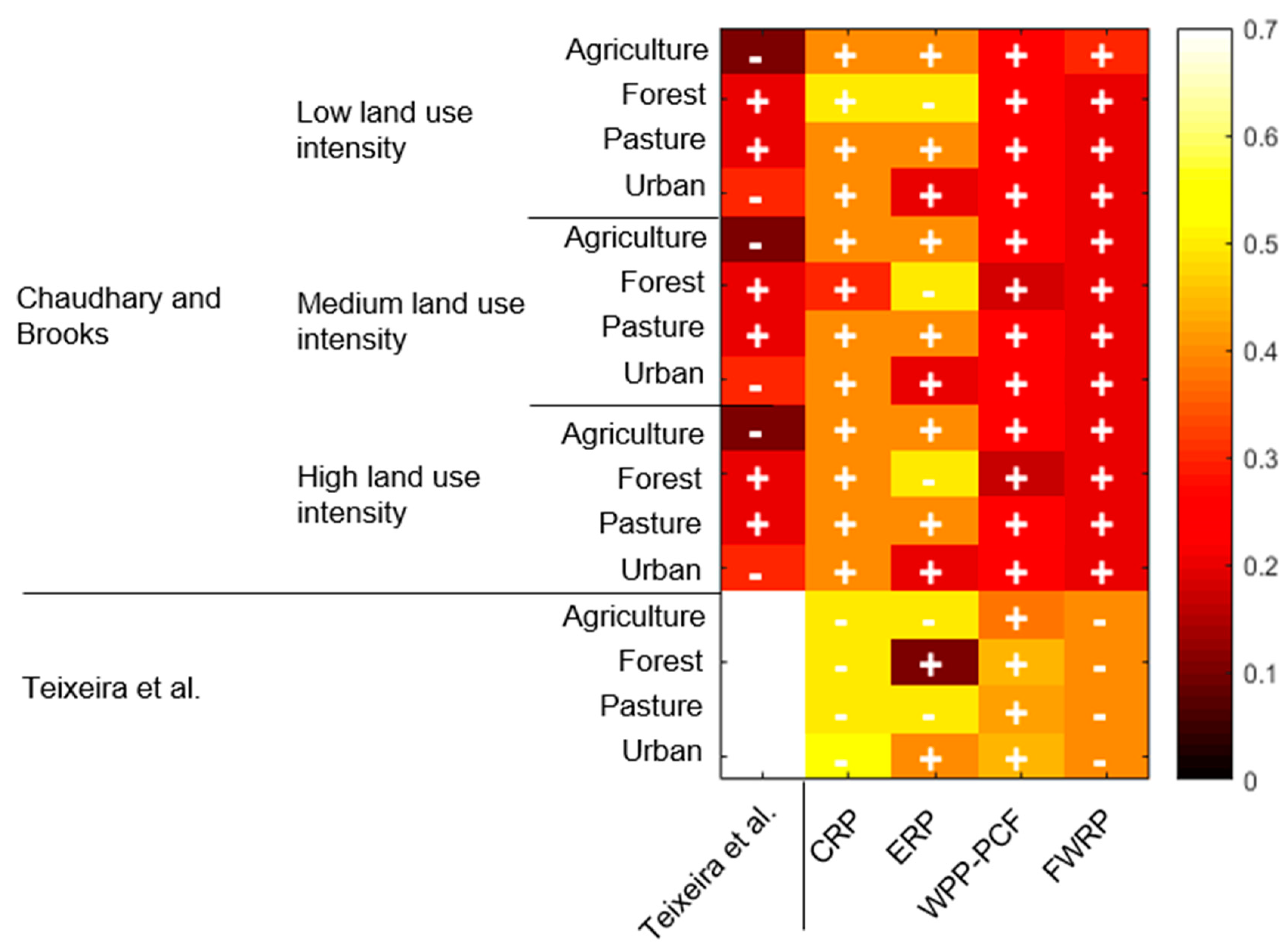
3.1. Correlation Analysis

The full list of correlation parameters between LCIA models is available in the Supplementary Material File S1. Results show four main groups of thematic indicators (where Spearman’s ρ is on average higher than 0.5 and significant at 1%). The first group included the ecosystem services indicators (Saad et al. [21], Müller-Wenk and Brandão [33] and LANCA [22]). The second group included SOC-based indicators (Brandão and Milà i Canals [15], Morais et al. [19] and Teixeira et al. [20]). The third included NPP/HANPP indicators (Alvarenga et al. [17], Alvarenga et al. [16] and Taelman et al. [18]), and finally the fourth group includes biodiversity methods (de Baan et al. [23], Chaudhary et al. [24] and Chaudhary and Brooks [25]).

Regarding the first group, water purification indicators (WPP-PCF and WPP-MF) address similar environmental areas but their correlation is only the second highest (average: 0.64 for Saad et al. [21] and 0.61 for LANCA [22]—regardless of the land use class for both methods). The correlations between Saad et al. [21] indicators are positive. For example, when the loss in WPP-PCF increases, losses in WPP-MF also increases, while correlations between LANCA [22] indicators are the opposite. For both indicators, Saad et al. [21] and the LANCA method [22] are poorly correlated (WPP-PCF average: 0.24; WPP-PCF: 0.29). Saad et al.’s [21] WPP-MF indicator is positively correlated with LANCA’s [22] WPP-MF, but for WPP-PCF the correlation is negative. These water purification indicators (WPP-MF and WPP-PCF) are poorly correlated with the groundwater recharge indicator (average: 0.17 between Saad et al. [21] indicators and 0.09 between LANCA method [22] indicators). The correlations between water purification indicators and groundwater recharge, for LANCA [22], is negative for forests and positive for all other land use classes. Considering all models in this first group, CRP and ERP from Saad et al. [21] are the indicators with higher correlations (average: 0.70—regardless of the land use class). For agriculture, pasture and urban land classes, the correlations are positive, but for the forest class the correlation is negative (i.e., when the losses in climate regulation are higher, the losses in erosion are lower).

SOC-based LCIA models are significant correlated, mainly between Brandão and Milà i Canals [15] and Morais et al. [19] (all correlations are above 0.5 for occupation and transformation CFs), followed by the correlations between Morais et al. [19] and Teixeira et al. [20]. The lowest correlations are between Brandão and Milà i Canals [15] and Teixeira et al. [20] (occupation average: −0.3; transformation average: −0.5). Almost all correlation between Brandão and Milà i Canals [15] and Teixeira et al. [20] are negative, i.e., when SOC depletion is high using Brandão and Milà i Canals [15] methods, the SOC depletion is low using Teixeira et al. [20]. Regardless of the models, correlations are higher in the “agriculture” class. In general, SOC-based models are more correlated in terms of their occupation CFs than transformation CFs. The average correlation between the occupation CFs is 0.44 (minimum: 0.003; maximum: 0.9), while the average correlation between transformation CFs is only 0.27 (minimum: 0.001; maximum: 0.9). For example, the occupation CFs of Morais et al. [19] and Teixeira et al. [20] are strongly and significantly correlated (0.45), but the correlation between the transformation CFs of both models is only 0.25. Transformation CFs are less correlated because they require an additional variable in their calculation, namely, the regeneration time. Distinct data and assumptions for the determination of this variable cause differences in the absolute values of the CFs and their regional distribution, even when occupation CFs are similar. For example, Morais et al. [19] used the same approach for SOC regeneration as Brandão and Milà i Canals [15], while Teixeira et al. [20] tested and then consolidated multiple ways to estimate the regeneration time.

Regarding NPP/HANPP indicators, Alvarenga et al. [17] and Alvarenga et al. [16] are strongly and significantly correlated (average: 0.81). However, correlations between Alvarenga et al. [17] and Taelman et al. [18] are negative and poorly correlated (average: −0.3). Alvarenga et al. [16] and Taelman et al. [18] are also poorly correlated, but the correlation is positive (average: 0.36). The correlations between SOC depletion models and HANPP/NPP are lower in absolute value, but significant at the 1% level of CFs. The correlations are higher for agriculture and lower for the forest land use class. The correlation between SOC-based models of Teixeira et al. [20] and Morais et al. [19] with HANNP/NPP-based models are negative (with some exceptions, but the correlation is close to zero, e.g., between Morais et al. [19] and Alvarenga et al. [16] for the urban land use class). The highest correlations are between Teixeira et al. [20] and Alvarenga et al. [17] (occupation average: 0.53), followed by the correlations between Brandão and Milà i Canals [15] and Alvarenga et al. [17] (occupation average: 0.46). The lowest correlations are between Morais et al. [19] and Alvarenga et al. [17] (occupation average: 0.10).

In the fourth and final group, which comprises biodiversity models, the correlations between all models are high and significant at 1%, regardless of the taxonomic group and land use class. All correlations are higher than 0.6 (both occupation and transformation CFs). The correlations for occupation CFs are slightly higher than the correlation for transformation CFs (occupation average: 0.8; transformation: 0.7). Highest correlations are found for agriculture, and the lowest for pasture. There are no significant differences between taxonomic groups.

Figure 1 presents the correlations for occupation CFs between some representative models of each group (i.e., SOC-based, Teixeira et al. [20]; ecosystem services, Saad et al. [21] complemented with Müller-Wenk and Brandão [33]; biodiversity, Chaudhary and Brooks [25]). The highest correlation is between CRP and SOC depletion in the urban land use class (0.55). The lowest correlation also involves SOC depletion models, but in this case with ERP for forests (0.13). Land use and biodiversity models are poorly and non-significantly correlated (for all land class intensities). Agriculture has the lowest correlations, while urban uses have the highest correlations (regardless of land use intensity).

Among all the taxonomic groups from Chaudhary and Brooks [25], correlations for plants are slightly higher than for other taxonomic groups, but not statistically significant for most land classes with high intensity of use. Further, agricultural and urbanized uses are negatively correlated, while naturalized land uses (forest and pasture) are positively correlated. The opposite was found for correlations between ERP and WPP-MF and biodiversity, where correlations for forest are negative. The correlations between CRP and Teixeira et al. [20] are the highest between the models in Figure 1, but they are negatively correlated. There is more spatial variation in Teixeira et al. [20] than in CRP (country CFs derived from seven biomes). SOC depletion is also highly correlated with ERP, for all land classes (except forests). CRP and ERP are the ecosystem services with highest correlations with the biodiversity CFs. Water purification and groundwater recharge are poorly correlated with biodiversity indicators (0.24). Their correlations with SOC depletion are higher (0.43).

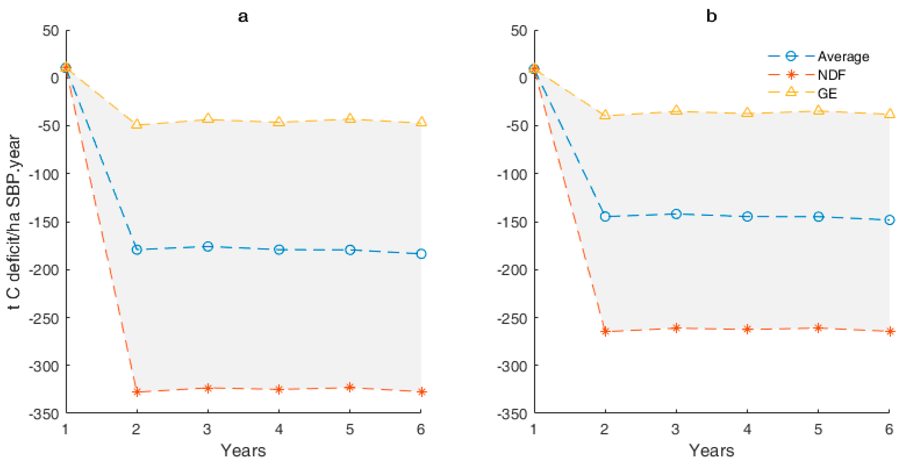
3.2. Case Study Results

The replacement of commercial feed with SBP in the first year requires on average 343 m²·year/ha of SBP per year of indirect land occupation. The sum of all transformation flows is 59 m²/ha of SBP per year, but some of these flows counteract each other as they have opposite signs (i.e., transformations from and to the same land use). In the first year, the second scenario (SBP + SNP) requires more land because the SBP cannot be fully grazed, in order to enable full pasture implementation and establishment of a resilient seed bank, and consequently feed is still required. In the following years, the scenario with SBP avoids the occupation of 4828 m²·year/ha SBP, or approximately 0.5 ha/ha SBP per year, and 10,200 m²/ha SBP per year of land transformation per hectare of SBP. The main contributor to the higher impact of the first scenario (SNP + commercial feed) is the occupation required by the production of feed ingredients. The total indirect area occupied is 887 m²·year/t of feed and the sum of all transformation flows is 1759 m²/t of feed (for high forage feed). Soybean meal is the feed ingredient with highest land occupation (264 m²·year/t of feed—30% of the total area occupied), while maize silage only uses 173 m²·year/t of feed (20%) despite representing 70% of the high forage feed composition (in mass). The indirect land occupied by SBP is 360 m²·year/ha of SBP. About 67% (240 m²·year/ha of SBP per year) is due to phosphorus fertilizer production and 10% (38 m²·year/ha of SBP) due to lime production. After the first year, in years when phosphorus fertilizer is applied, land occupation is 149 m²·year/ha of SBP per year, and 49 m²·year/ha of SBP in the years with lime application. Regarding the indirect land transformation due to SBP installation, it is only 59 m²·year/ha of SBP per year (20% due to superphosphate production).

The application of the LCIA models to these inventory flows showed that the difference between the impacts of the two scenarios was always qualitatively similar. In the first year the difference of impacts is positive, meaning higher impacts caused by the SBP + SNP scenario than the baseline scenario. This is because the SBP installation requires more indirect land use flows than the annual tillage of SNP, and feed used is the same. The main sources of impact in SBP installation are phosphorus fertilizer and application of lime. In the second and following years, it is the baseline scenario that has higher impacts (for all LCIA models). The installation of SBP avoids the high impacts of feed production and consumption, which are always higher than the impact of any management operation on SBP (phosphorus fertilizer and lime application). The main source of impact (according to all models) of the commercial feeds are cereals grains and soybean meal (main source of land use impact). The full list of case study results (for all methods) is available in Supplementary Material File S2.

Figure 2 depicts results using Teixeira et al. [20] (as an example) for the difference between scenarios considering high forage feed. The SOC depletion potential due to occupation and transformation is on average −180 t C/ha of SBP per year (in the second and following years) and in the first year SOC depletion due to occupation and transformation is 10 t C/ha of SBP per year. Results with other SOC depletion methods are qualitatively similar but there are large differences in absolute values due to the differences in the CFs of the different models. For example, the world average occupation CF of Teixeira et al. [20] is 23 kg C deficit/m² (in the simple average aggregation) and 32 kg C deficit/m² (in the weighted average aggregation), while the ILCD [37] occupation CF for agricultural occupation in 9.8 kg C deficit/m².

Regarding the distribution of impacts between land occupation and transformation, on average, most of impact is due to occupation (land occupation is 75% of the total impact on average—for the different methods and indicators). When transformation inventory flows are translated into impacts, there are opposite flows that cancel each other during LCIA (e.g., “transformation to annual crop” and “transformation from annual crop”).

The regionalization of the first tier of the inventory changed 67% (598 m²·year/ha of SBP per year) of the area occupied, and 71% of the transformation flows (1248 m²/ha of SBP per year). From the first approach (non-regionalized inventory) to the second approach (regionalized approach), the origin of the main source of land occupation, i.e., soybean meal, remained the same (Brazil). Regarding SBP installation, the land occupation and transformation change was only 5% (due to the small weight of the seeds). Land occupation and transformation of SBP maintenance are not affected by the inventory regionalization as no intervening processes were affected. The same is true for SNP system (only one annual tillage operation).

Despite these significant changes in the origin of the inventory flows, the consequences for LCIA were relatively small. On average, further regionalization of inventory flows reduced the difference between scenarios by 15% (considering all models). For Teixeira et al. [20], the difference is shown in Figure 2b. Teixeira et al. [20] is the case where inventory regionalization affected the difference of scenarios the most, namely 18% in the first year and 23% in the second and following years. Even in this case, the change in results is smaller than the variation due to the use of different nutritional indicators to establish the equivalence between scenarios. Chaudhary and Brooks [25] is the least affected model, as results change only 5%, because most of the inventory flows for the feed are “high land use intensity” and the CFs are always high, regardless of where the occupation and transformation occur, and the relative differences are smaller. Regarding specific processes, feed inventory regionalization increases the impacts 13%. It reduces the impacts of SBP installation 10% due to the weight of the seeds (the only product regionalized in SBP installation) in the total impact.

4. Discussion

The main goal of this paper was to perform a practical test of all the LCIA models that are available and free to use. Rather than repeating the work done by institutions such as the European Commission or UNEP/SETAC of assessing the assumptions and methods of the models, we made a practical comparison of CFs and evaluated a case study where we applied those CFs.

4.1. Correlation Analysis

Our results suggest some spatial redundancy between models that depict the same environmental effects. For example, Chaudhary et al. [24] and Chaudhary and Brooks [25] (regardless of the land use and land use intensity) are very spatially correlated because the second model is an updated version of the first, whose main goal was to introduce land use intensity; however, the hotspots of impact are mostly the same. This is also true for de Baan et al. [23]. In all biodiversity methods, Central America and the Caribbean regions are where biodiversity loss is highest (e.g., Trinidad and Tobago has the highest occupation CF for mammal loss from agricultural occupation according to de Baan [23], the seventh according Chaudhary et al. [24] and fifteenth according to Chaudhary and Brooks [25]). In general, the highest CFs are found in the equatorial region. Results also show strong and significant correlations between some models that address different environmental aspects, as, for example, CRP from Müller-Wenk and Brandão [33] and Chaudhary and Brooks [25]. Country CFs of CRP at country scale were calculated at the scale of seven highly aggregated biomes. When disaggregated by country, the highest CFs are for the same countries highlighted by biodiversity models (e.g., Trinidad and Tobago is in the top twenty countries with highest CFs for agriculture).

In other cases, there seems to be strong complementarity between models as correlations are small or even non-existing. At high altitudes, CFs for biodiversity are typically low but SOC-based CFs are high, leading to low correlations between the models. Also, the Mediterranean region is one hotspot of species loss, while the lowest CFs in Morais et al. [19] are in this region due to the low SOC concentrations in this region (in all land use classes)—meaning that there is not much SOC to lose after land transformation. This also affects the correlations with Teixeira et al. [20]. Overall, the hotspots of SOC depletion are in different regions than the hotspots of biodiversity loss. The equatorial regions (e.g., sub-Saharan region) have the lowest SOC depletion in Teixeira et al. [20]. The hotspots of impact on SOC depletion are in the high latitude regions, where soil carbon stocks are the highest in potential natural vegetation. This is not an artifact of the models, but rather a plausible depiction of the fact that SOC depletion and biodiversity loss are not redundant effects.

The spatial correlation method used here only assesses if the relative distribution of the CFs for each country in the world and in each land class is similar for the different models. The correlation is high if the same regions have the highest CFs for any two models. Naturally, this is only one aspect that helps determine complementarity or redundancy between models. Our method does not assess methodological choices of each individual model, and no conclusion can be drawn about the accuracy of absolute values of the CFs, which, in many cases, vary considerably even for similar indicators. Significant correlation does not mean that there are no differences in absolute value. For example, occupation CFs from Morais et al. [19] are strongly and significantly related to Teixeira et al. [20], but in absolute values the CFs from Morais et al. [19] are about half of the CFs of Teixeira et al. [20]. Note that results of the correlations may have been affected by the aggregation that was needed for land classes and regions (conversion to country-level CFs), but not by the scale of the CFs. We performed the analysis using the actual reported CFs, but also tried depicting them in a normalized scale between −1 and 1 to avoid the influence of large differences in absolute values. Results, however, did not change.

It is unclear whether more LCIA model regionalization would lead to an increase in the correlation between methods. The fact that, regardless of the differences pointed out, most models of each group are spatially very correlated means that the geographical distribution of impacts is basically unchanged in all models. Geospatial distribution is only affected by impact pathway covered and indicator used (species loss, SOC depletion, etc.), not by modelling choices.

However, correlations are very different depending on the land class. This suggests that land classes should be the main determinant in improving model performance going forward. The inclusion of more land classes will introduce more detail into the CFs and seems to be a more promising development path for models than simply adding more geospatial detail. The problem is that there may be a trade-off between having more land classes or regionalization [19]. There is typically a lack of measured data for all potential land desirable classes modelled to produce the CFs. Process-based models can potentially be used to overcome this trade-off. These models can overcome data limitations on the variables of interest (species, SOC, etc.) by estimating them using auxiliary (and easier to source) data that can remain site specific (e.g., dependence on soil properties), depend on climate conditions (temperature, precipitation and evaporation) and is based on scenarios. For SOC-based indicators this was illustrated by Morais et al. [60], who proposed an LCIA method using the Rothamsted Carbon model to calculate occupation and transformation CFs for more than 1000 small sub-regions within the region of Alentejo in Portugal. Morais et al. [60] were capable of calculating CFs for 23 land classes, including 16 agricultural classes corresponding to individual crops. Besides increasing the number of land classes, these models can also assist in the production of CFs that reflect land use intensity and even management operations, particularly for crops. Nevertheless, increasing the number of land use classes creates new challenges in terms of inventory. The available background databases only consider aggregated land occupation and transformation flows, although there is more information on inventory processes that can be used and matched with the applicable CF.

As a final note regarding the correlation analysis, the indicators of the land use and biodiversity models used in this study are different but related according to the impact pathway proposed by Koellner et al. [40]. According to this pathway, for example, SOC is one midpoint indicator leading to ecosystem services damage potential (endpoint), as are CRP and ERP. Therefore, the models assessed were expected to be related (e.g., SOC depletion should be related to species loss and HANPP should be related do BPP). This theoretical expectation is indeed verified, but even statistically significant correlations are far from 1 (perfect correlation). This lack of perfect redundancy was also expected, as different models target particular elements of the land use impact pathway.

4.2. Case Study Results

In the second part of the results, we applied the CFs produced by all models to a case study for meat production, namely the substitution of feed for SBP. This case study served as a demonstrative application of the characterization models, but its results are important regardless of this context. There is a lack of agri-food LCA studies in Portugal, and the ones available typically disregard land use impacts, for example, on biodiversity [61]. We applied CFs based on the region where the inventory processes used take place as stated in ecoinvent, but we also tested the consequences of assigning those flows to the country where they are known to take place. Results showed that this extra inventory regionalization changed approximately 70% of the inventory flows, as the most significant first-tier processes were affected, but then LCIA results only changed by 15% on average and 23% at the most. The specification of where the processes occur did not seem to produce a change in results of the same magnitude of the representativeness of the flows changed. Consequently, this extra step seemed not to make a definitive difference in results, which again highlights that more regionalization may not be crucial to obtain improved estimations of the impacts of land use.

These results, however, must be understood on the basis of the models that are available and their relatively coarse scale. If inventory flows and CFs were depicted at a scale smaller than the country, the consequences for LCIA results could become more relevant due to potential higher variability of the CFs at smaller scales. Countries usually are an aggregation of multiple regions (some with higher CFs and others with low CFs) which tend to make the spatial distribution of CFs uniform. Furthermore, in other applications and case studies, the relevance of the inventory could be more significant, namely if the land occupation or the transformation took place in a country that was less representative of the larger region in which it is integrated (e.g., a country with a particularly low CF within a region with a significantly higher CF), which is not the case in this case study.

Additionally, all models presented qualitatively similar results for the comparisons between scenarios. Regardless of the inventory approach or LCIA model, we always concluded that feed substitution with SBP leads to avoided impact, except in the first year. Nevertheless, depending on the method used, the absolute value of the results change considerably (e.g., Teixeira et al. [20] leads to an estimation of the avoided impact, measured in terms of SOC depletion, one order of magnitude higher that the results from Brandão and Milà i Canals [15]). These results suggest that although the particular features of the models, such as underlying framework, data or other modelling choices produce high geographical agreement, the actual estimated impact in absolute terms can change dramatically between models.

Here, direct land occupation impacts were disregarded due to the scenario equivalence. If they had been included (i.e., the CF for the occupation of 1 ha·year of pasture), there would be a lack of differentiation between pastures types in the CFs. Potentially the CFs from Chaudhary and Brooks [25] could be used if one assumed that SBP are high intensity use and SNP low intensity. The low intensity land use CF would be 3.09 × 10⁻⁹ potential plants loss/m² and the high intensity land use CF would be 4.07 × 10⁻⁹ potential plants loss/m² for the ecoregion that includes the region of Alentejo, where most SBP are located. As the CF for high intensity pasture use is higher, the conclusion would be that SBP have more direct impacts on biodiversity. There is, however, some empirical evidence for birds and anthropoids that suggests otherwise—namely, that biodiversity would be unaffected from the change [47]. This highlights a structural problem with using “intensity”, a vague concept with very distinct interpretations that depend strongly on the actual management practices. As for SOC-based indicators, no distinction between scenarios would be possible. The average avoided impact for high forage feed is about −180 t C deficit per hectare of SBP per year (Figure 2), using Teixeira et al. [20]. Using the same method, the occupation of one hectare of pasture represents about 148 t C deficit per year—which means that, overall, the results would still be negative (gain in SOC). Nevertheless, the direct land use occupation impact is only 5% of the total impact of SBP installation and about 10% in the following years with phosphorus or lime application (in years without management operations the only impact would be the direct land use occupation, i.e., 100% of the impact).

4.3. Outlook and Future Developments

Our results show some indication that regionalization may not be the main issue in LCIA currently due to the good spatial agreement between comparable models and the lack of spatial detail available in inventories to match the spatial detail of the most advanced LCIA models. We showed that adding more country-level regionalization to inventories, and using country-level CFs rather than continental or global CFs, does not change results significantly. These two observations may be a co-effect of the reliance of inventories on the country-scale. For economic reasons, countries are a welcome and useful division of the world. For biophysical effects, such as the impacts from land use, they are not particularly useful. It would be important to test, due to country aggregation issues, the effects of inventories becoming regionalized beyond the country scale, and whether the application of CFs at lower scales to those inventory flows would produce more asymmetrical spatial patterns. It is possible that if we had been able to disaggregate the inventory at a lower scale than the country, the differences between the application of regional CFs and global CFs would be larger.

In spite of the achievements in the methods assessed in this paper, two aspects can still be improved. The first and most pressing issue seems to be increasing the number of land use classes (e.g., specific crops rather than an “agriculture” class). The second welcome development is the development of disaggregated CFs for each land class that differentiate production systems and management operations (e.g., no-till irrigated maize rather just one CF for maize). Regarding the first issue, only one method desegregated “agriculture”, for example, into two agricultural classes (annual and permanent classes—de Baan et al. [23]) and only one into more than two classes (Alvarenga et al. [16]). All other methods considered only one agricultural class. This is a critical failure in global LCIA land use models and as such should be given priority. Regarding the second issue, the problem runs deeper because the issue of production systems is sometimes reduced to a simple difference in “land use intensity”. Two methods differentiate between land use intensity, namely Chaudhary and Brooks [25] and LANCA [22]. However, “intensity” is an abstract concept that has different implications depending on the type of land use and the region. High-intensity pasture use can mean drastically different things in the British Isles and in the Mediterranean. The LCIA community should make their view of “intensity” more complex, as the effects of intensification on biotic production and biodiversity may not be linear. Intensity should be explicitly connected with management practices, whose effects are also regional.

The case study presented here offers some insights, but they are limited by the fact that it is a single case. Results obtained can be highly influenced by the specificities of the application example. Characterization models must be stress tested in multiple situations and scenarios, to demonstrate their flexibility and comprehensiveness. LCIA models lack an application, with developers offering only simple and almost academic illustrations of their methods in papers (in some cases considering only direct impacts rather than complete supply chains). These applications usually are not as comprehensive as the one presented here, as they select one method or one method per environmental issue, and never present true comparisons. There are some exceptions, as for example an assessment of land use and biodiversity impacts of breakfast cereals [62]. Methodological studies about model assumptions are more common, as, for example, evaluations of the role of the reference state in LCIA [26]. It is important to test the models for multiple products from multiple sectors and regions, as results can change between indicators to some degree, particularly for agri-food products [63]. It is also important to move CFs beyond simple statistical data evaluations and make them more realistic, evidence-based and related to actually modelled effects on ecosystems. Complex systems such as multifunctional pastures could lead to ecosystem services and biodiversity benefits [9,46,64], but CFs today do not translate that fact (for direct effects).

5. Conclusions

LCA practitioners require guidance for the application of impact assessment models, whose development has proliferated in the recent past. Consensus between experts is the most common way found of arriving at single and reliable recommendations, but the process for reaching a consensus does not always consider the practical issues of trying to apply the model. Future consensus-building initiatives should also consider the consequences of recommending specific models when those are applied in practical studies. This was our motivation for the work presented here, which showed how practical application cases can provide valuable insights about the nature of models and their needed future directions. We found good spatial agreement between models that use similar indicators, but significant variation depending on the land class. We found that, when these indicators are applied to pasture-based meat production, they provide the same qualitative conclusions for comparatively assessing scenarios. The installation of each hectare of sown pastures saves approximately 0.5 hectares of land that would have been needed to produce the feeds replaced; it also avoids SOC depletion and loss of species. However, these models would be either unable or unreliable to determine the direct plot-level effects of management of specific pasture systems. LCIA models that offer CFs based on “intensity”, if applied to one hectare of each pasture system, would assume higher impacts of SBP simply due to being more productive—but there is no evidence of this effect being real.

We therefore recommend as future directions for LCIA models that: (a) the development of land class-specific CFs is given priority over more regionalization of effects, because at the country level similar models agree on the relative spatial distribution of impacts and because more spatial detail at LCIA level would be difficult to match at inventory level; (b) when more regionalization is used, particularly at inventory level, developers move away from countries as the basic territorial unit, because they are an inaccurate homogeneous region for the assessment of biophysical effects; (c) model developers move beyond the simple assessment of “land use intensity”, which is a vague concept, and actually add land classes that are a function of management and, through the effect of management on local ecosystems, have a strong regional component; and, (d) LCIA models are more frequently tested in comparative settings with complex supply chains involved, such as the one presented here, rather than in basic academic examples.

References

1. Hellweg, S.; Milà i Canals, L. Emerging approaches, challenges and opportunities in life cycle assessment. Science 2014, 344, 1109–1113. [Google Scholar] [CrossRef] [PubMed]
2. Roy, P.; Nei, D.; Orikasa, T.; Xu, Q.; Okadome, H.; Nakamura, N.; Shiina, T. A review of life cycle assessment (LCA) on some food products. J. Food Eng. 2009, 90, 1–10. [Google Scholar] [CrossRef]
3. Foster, C.; Green, K.; Bleda, M.; Dewik, P. Environmental Impacts of Food Production and Consumption: Final Report to the Department for Environment Food and Rural Affairs; Food and Agriculture Organization (FAO): Rome, Italy, 2007. [Google Scholar]
4. Notarnicola, B.; Hayashi, K.; Curran, M.A.; Huisingh, D. Progress in working towards a more sustainable agri-food industry. J. Clean. Prod. 2012, 28, 1–8. [Google Scholar] [CrossRef]
5. Teixeira, R.F.M. Critical Appraisal of Life Cycle Impact Assessment Databases for Agri-food Materials. J. Ind. Ecol. 2015, 19, 38–50. [Google Scholar] [CrossRef]
6. Teixeira, R.; Himeno, A.; Gustavus, L. Carbon footprint of breton pâté production: A case study. Integr. Environ. Assess. Manag. 2013, 9, 645–651. [Google Scholar] [CrossRef] [PubMed]
7. Morais, T.G.; Teixeira, R.F.M.; Rodrigues, N.R.; Domingos, T. Carbon footprint of milk from pasture-based dairy farms in Azores, Portugal. Sustainability 2018, 10, 3658. [Google Scholar] [CrossRef]
8. De Vries, M.; de Boer, I.J.M.J.M. Comparing environmental impacts for livestock products: A review of life cycle assessments. Livest. Sci. 2010, 128, 1–11. [Google Scholar] [CrossRef]
9. Chatterton, J.; Graves, A.; Audsley, E.; Morris, J.; Williams, A. Using systems-based life cycle assessment to investigate the environmental and economic impacts and benefits of the livestock sector in the UK. J. Clean. Prod. 2015, 86, 1–8. [Google Scholar] [CrossRef]
10. Nguyen, T.L.T.; Hermansen, J.E.; Mogensen, L. Environmental consequences of different beef production systems in the EU. J. Clean. Prod. 2010, 18, 756–766. [Google Scholar] [CrossRef]
11. Teixeira, R.F.M. The cost-effectiveness of optimizing concentrated feed blends to decrease greenhouse gas emissions. Environ. Eng. Manag. J. 2018, 17, 999–1007. [Google Scholar] [CrossRef]
12. Vidal Legaz, B.; Maia De Souza, D.; Teixeira, R.F.M.; Antón, A.; Putman, B.; Sala, S. Soil quality, properties, and functions in life cycle assessment: An evaluation of models. J. Clean. Prod. 2017, 140, 502–515. [Google Scholar] [CrossRef]
13. Souza, D.M.; Teixeira, R.F.M.; Ostermann, O.P. Assessing biodiversity loss due to land use with Life Cycle Assessment: Are we there yet? Glob. Chang. Biol. 2015, 21, 32–47. [Google Scholar] [CrossRef] [PubMed]
14. Morais, T.G.; Domingos, T.; Teixeira, R.F.M. Are land use and biodiversity midpoint indicators redundant or complementary? In Proceedings of the Conference on Life Cycle Assessment in the Agri-Food Sector, Dublin, Ireland, 19–21 October 2016; American Center for Life Cycle Assessment: Dublin, Ireland, 2016. [Google Scholar]
15. Brandão, M.; Milà i Canals, L. Global characterisation factors to assess land use impacts on biotic production. Int. J. Life Cycle Assess. 2013, 18, 1243–1252. [Google Scholar] [CrossRef]
16. Alvarenga, R.A.F.; Erb, K.-H.; Haberl, H.; Soares, S.R.; van Zelm, R.; Dewulf, J. Global land use impacts on biomass production—A spatial-differentiated resource-related life cycle impact assessment method. Int. J. Life Cycle Assess. 2015, 20, 440–450. [Google Scholar] [CrossRef]
17. Alvarenga, R.A.F.; Dewulf, J.; Van Langenhove, H.; Huijbregts, M.A.J. Exergy-based accounting for land as a natural resource in life cycle assessment. Int. J. Life Cycle Assess. 2013, 18, 939–947. [Google Scholar] [CrossRef]
18. Taelman, S.E.; Schaubroeck, T.; De Meester, S.; Boone, L.; Dewulf, J. Accounting for land use in life cycle assessment: The value of NPP as a proxy indicator to assess land use impacts on ecosystems. Sci. Total Environ. 2016, 550, 143–156. [Google Scholar] [CrossRef] [PubMed]
19. Morais, T.G.; Domingos, T.; Teixeira, R.F.M. A spatially explicit life cycle assessment midpoint indicator for soil quality in the European Union using soil organic carbon. Int. J. Life Cycle Assess. 2016, 21, 1076–1091. [Google Scholar] [CrossRef]
20. Teixeira, R.F.M.; Morais, T.G.; Domingos, T. Consolidating regionalized global characterization factors for soil organic carbon depletion due to land occupation and transformation. Environ. Sci. Technol. 2018. [Google Scholar] [CrossRef] [PubMed]
21. Saad, R.; Koellner, T.; Margni, M. Land use impacts on freshwater regulation, erosion regulation, and water purification: A spatial approach for a global scale level. Int. J. Life Cycle Assess. 2013, 18, 1253–1264. [Google Scholar] [CrossRef]
22. Bos, U.; Horn, R.; Beck, T.; Lindner, J.P.; Fischer, M. LANCA®—Characterization Factors for Life Cycle Impact Assessment, Version 2.3; Fraunhofer Verlag: Stuttgart, Germany, 2016. [Google Scholar]
23. De Baan, L.; Mutel, C.L.; Curran, M.; Hellweg, S.; Koellner, T. Land use in life cycle assessment: Global characterization factors based on regional and global potential species extinction. Environ. Sci. Technol. 2013, 47, 9281–9290. [Google Scholar] [CrossRef] [PubMed]
24. Chaudhary, A.; Verones, F.; de Baan, L.; Hellweg, S. Quantifying Land Use Impacts on Biodiversity: Combining Species-Area Models and Vulnerability Indicators. Environ. Sci. Technol. 2015, 49, 9987–9995. [Google Scholar] [CrossRef] [PubMed]
25. Chaudhary, A.; Brooks, T.M. Land Use Intensity-specific Global Characterization Factors to Assess Product Biodiversity Footprints. Environ. Sci. Technol. 2018, 52, 5094–5104. [Google Scholar] [CrossRef] [PubMed]
26. Cao, V.; Margni, M.; Favis, B.D.; Deschênes, L. Choice of land reference situation in life cycle impact assessment. Int. J. Life Cycle Assess. 2017, 22, 1220–1231. [Google Scholar] [CrossRef]
27. European Commission—Joint Research Centre; Institute for Environment and Sustainability. International Reference Life Cycle Data System (ILCD) Handbook: Analysing of Existing Environmental Impact Assessment Methodologies for Use in Life Cycle Assessment; European Commission: Brussels, Belgium, 2010. [Google Scholar]
28. Jolliet, O.; Frischknecht, R.; Bare, J.; Boulay, A.-M.; Bulle, C.; Fantke, P.; Gheewala, S.; Hauschild, M.; Itsubo, N.; Margni, M.; et al. Global guidance on environmental life cycle impact assessment indicators: Findings of the scoping phase. Int. J. Life Cycle Assess. 2014, 19, 962–967. [Google Scholar] [CrossRef]
29. Jolliet, O.; Müller-Wenk, R.; Bare, J.; Brent, A.; Goedkoop, M.; Heijungs, R.; Itsubo, N.; Peña, C.; Pennington, D.; Potting, J.; et al. The LCIA midpoint-damage framework of the UNEP/SETAC life cycle initiative. Int. J. Life Cycle Assess. 2004, 9, 394–404. [Google Scholar] [CrossRef] [Green Version]
30. Teixeira, R.F.M.; Maia de Souza, D.; Curran, M.P.; Antón, A.; Michelsen, O.; Milà i Canals, L. Towards consensus on land use impacts on biodiversity in LCA: UNEP/SETAC Life Cycle Initiative preliminary recommendations based on expert contributions. J. Clean. Prod. 2016, 112, 4283–4287. [Google Scholar] [CrossRef]
31. Curran, M.; de Souza, D.M.; Antón, A.; Teixeira, R.F.M.; Michelsen, O.; Vidal-Legaz, B.; Sala, S.; Milà i Canals, L. How Well Does LCA Model Land Use Impacts on Biodiversity?—A Comparison with Approaches from Ecology and Conservation. Environ. Sci. Technol. 2016, 50, 2782–2795. [Google Scholar] [CrossRef] [PubMed]
32. Valada, T.; Teixeira, R.F.; Domingos, T. Environmental and energetic assessment of sown irrigated pastures vs. maize. In Sustainable Mediterranean Grasslands and Their Multi-Functions; Options Méditerranéennes Série A: Séminaires Méditerranéens; CIHEAM/FAO/ENMP/SPPF: Zaragoza, Spain, 2008; No. 79; pp. 131–134. [Google Scholar]
33. Müller-Wenk, R.; Brandão, M. Climatic impact of land use in LCA—Carbon transfers between vegetation/soil and air. Int. J. Life Cycle Assess. 2010, 15, 172–182. [Google Scholar] [CrossRef]
34. De Souza, D.M.; Flynn, D.F.B.; DeClerck, F.; Rosenbaum, R.K.; de Melo Lisboa, H.; Koellner, T. Land use impacts on biodiversity in LCA: Proposal of characterization factors based on functional diversity. Int. J. Life Cycle Assess. 2013, 18, 1231–1242. [Google Scholar] [CrossRef]
35. Cao, V.; Margni, M.; Favis, B.D.; Deschênes, L. Aggregated indicator to assess land use impacts in life cycle assessment (LCA) based on the economic value of ecosystem services. J. Clean. Prod. 2015, 94, 56–66. [Google Scholar] [CrossRef]
36. Wernet, G.; Bauer, C.; Steubing, B.; Reinhard, J.; Moreno-Ruiz, E.; Weidema, B. The ecoinvent database version 3 (part I): Overview and methodology. Int. J. Life Cycle Assess. 2016, 21, 1218–1230. [Google Scholar] [CrossRef]
37. Milà i Canals, L.; Muñoz, I.; McLaren, S.; Brandão, M. LCA Methodology and Modelling Considerations for Vegetable Production and Consumption; CES Working Papers 02/07; Centre for Environmental Strategy, University of Surrey: Surrey, UK, 2007. [Google Scholar]
38. European Commission—Joint Research Centre; Institute for Environment and Sustainability. International Reference Life Cycle Data System (ILCD) Handbook—Recommendations for Life Cycle Impact Assessment in the European Context; Publications Office of the European Union: Luxemburg, 2011; ISBN 9789279174513. [Google Scholar]
39. Tóth, G.; Jones, A.; Montanarella, L. The LUCAS topsoil database and derived information on the regional variability of cropland topsoil properties in the European Union. Environ. Monit. Assess. 2013, 185, 7409–7425. [Google Scholar] [CrossRef] [PubMed]
40. Koellner, T.; Baan, L.; Beck, T.; Brandão, M.; Civit, B.; Margni, M.; Milà i Canals, L.; Saad, R.; De Souza, D.M.; Müller-Wenk, R. UNEP-SETAC guideline on global land use impact assessment on biodiversity and ecosystem services in LCA. Int. J. Life Cycle Assess. 2013, 18, 1188–1202. [Google Scholar] [CrossRef] [Green Version]
41. Pereira, H.M.; Ziv, G.; Miranda, M. Countryside species-area relationship as a valid alternative to the matrix-calibrated species-area model. Conserv. Biol. 2014, 28, 874–876. [Google Scholar] [CrossRef] [PubMed]
42. Spearman, C. The Proof and Measurement of Association between Two Things. Am. J. Psychol. 1904, 15, 72–101. [Google Scholar] [CrossRef]
43. Teixeira, R.F.M.; Proença, V.; Crespo, D.; Valada, T.; Domingos, T. A conceptual framework for the analysis of engineered biodiverse pastures. Ecol. Eng. 2015, 77, 85–97. [Google Scholar] [CrossRef]
44. Teixeira, R.F.M.; Domingos, T.; Costa, A.P.S.V.; Oliveira, R.; Farropas, L.; Calouro, F.; Barradas, A.M.; Carneiro, J.P.B.G. The dynamics of soil organic matter accumulation in Portuguese grasslands soils. In Sustainable Mediterranean Grasslands and Their Multi-Functions; CIHEAM/FAO/ENMP/SPPF: Zaragoza, Spain, 2008; pp. 41–44. [Google Scholar]
45. Teixeira, R.F.M.; Domingos, T.; Canaveira, P.; Avelar, T.; Basch, G.; Belo, C.C.; Calouro, F.; Crespo, D.; Ferreira, V.G.; Martins, C. Carbon sequestration in biodiverse sown grasslands. In Sustainable Mediterranean Grasslands and Their Multi-Functions; CIHEAM/FAO/ENMP/SPPF: Zaragoza, Spain, 2008; pp. 123–126. [Google Scholar]
46. Teixeira, R.F.M.; Domingos, T.; Costa, A.P.S.V.; Oliveira, R.; Farropas, L.; Calouro, F.; Barradas, A.M.; Carneiro, J.P.B.G. Soil organic matter dynamics in Portuguese natural and sown rainfed grasslands. Ecol. Model. 2011, 222, 993–1001. [Google Scholar] [CrossRef]
47. Teixeira, R.F.M. Sustainable Land Uses and Carbon Sequestration: The Case of Sown Biodiverse Permanent Pastures Rich in Legumes. Ph.D. Thesis, Instituto Superior Técnico, Lisboa, Portugal, 2010. [Google Scholar]
48. Teixeira, R.F.M.; Barão, L.; Morais, T.G.; Domingos, T. “BalSim”: A carbon, nitrogen and greenhouse gas mass balance model for pastures. Sustainability 2018. under revision. [Google Scholar]
49. Teixeira, R.; Pax, S. A Survey of Life Cycle Assessment Practitioners with a Focus on the Agri-Food Sector. J. Ind. Ecol. 2011, 15, 817–820. [Google Scholar] [CrossRef]
50. Pereira, H.M.; Domingos, T.; Marta-Pedroso, C.; Proença, V.; Rodrigues, P.; Ferreira, M.; Teixeira, R.; Mota, R.; Nogal, A. Uma avaliação dos serviços dos ecossistemas em Portugal. In Ecossistemas e Bem-Estar Humano Avaliação para Portugal do Millennium Ecosystem Assessment; Escolar Editora: Lisboa, Portugal, 2009; pp. 687–716. [Google Scholar]
51. Morais, T.G.; Teixeira, R.F.M.; Domingos, T. The effects on greenhouse gas emissions of sustainable intensification of meat production with rainfed sown biodiverse pastures. Sustainability 2018. under revision. [Google Scholar]
52. International Organization for Standardization (ISO). 14040 Environmental Managemente Life Cycle Assessmente Principles and Framework; International Organization for Standardization: Geneva, Switzerland, 2006. [Google Scholar]
53. Gabinete de Planeamento e Política (GPP). Contas de Cultura das Actividades Vegetais, Ano 1997—Modelo de Base Microeconómica (“Crop Sheets 1997—Microeconomic Base Model”, in Portuguese); Ministério da Agricultura, do Desenvolvimento Rural e das Pescas—Gabinete de Planeamento e Política Ago-Alimentar: Lisbon, Portugal, 2001. [Google Scholar]
54. Weidema, B.P.; Bauer, C.; Hischier, R.; Mutel, C.; Nemecek, T.; Reinhard, J.; Vadenbo, C.O.; Wernet, G. Overview and Methodology. Data Quality Guideline for the Ecoinvent Database Version 3; Ecoinvent Report 1 (v3); Swiss Centre for Life Cycle Inventories: St. Gallen, Switzerland, 2013. [Google Scholar]
55. Costa, P.; Lemos, J.P.; Lopes, P.A.; Alfaia, C.M.; Costa, A.S.H.; Bessa, R.J.B.; Prates, J.A.M. Effect of low- and high-forage diets on meat quality and fatty acid composition of Alentejana and Barrosã beef breeds. Animal 2012, 6, 1187–1197. [Google Scholar] [CrossRef] [PubMed] [Green Version]
56. Morais, T.G.; Teixeira, R.F.; Domingos, T. A step toward regionalized scale-consistent agricultural life cycle assessment inventories. Integr. Environ. Assess. Manag. 2017, 13, 939–951. [Google Scholar] [CrossRef] [PubMed]
57. L’Agence de l’Environnement et de la Maîtrise de l’Energie (ADEME). AGRIBALYSE®: Rapport Méthodologique—Version 1.0; ADEME: Angers, France, 2013. [Google Scholar]
58. Nemecek, T.; Bengoa, X.; Lansche, J.; Mouron, P.; Rossi, V.; Humbert, S. Methodological Guidelines for the Life Cycle Inventory of Agricultural Products; Version 2.0; World Food LCA Database (WFLDB): Lausanne/Zurich, Switzerland, 2014. [Google Scholar]
59. Industriais de Alimentos Compostos para Animais (IACA). Anuário 2017; Portuguese Association of Producers of Commercial Feeds for Animals, Associação Portuguesa dos Industriais de Alimentos Compostos para Animais: Lisbon, Portugal, 2017. (In Portuguese) [Google Scholar]
60. Morais, T.G.; Silva, C.; Jebari, A.; Álvaro-Fuentes, J.; Domingos, T.; Teixeira, R.F.M. A proposal for using process-based soil models for land use Life cycle impact assessment: Application to Alentejo, Portugal. J. Clean. Prod. 2018, 192, 864–876. [Google Scholar] [CrossRef]
61. Morais, T.G.; Teixeira, R.F.M.; Domingos, T. Regionalization of agri-food life cycle assessment: A review of studies in Portugal and recommendations for the future. Int. J. Life Cycle Assess. 2016, 21, 875–884. [Google Scholar] [CrossRef]
62. Jeswani, H.K.; Hellweg, S.; Azapagic, A. Accounting for land use, biodiversity and ecosystem services in life cycle assessment: Impacts of breakfast cereals. Sci. Total Environ. 2018, 645, 51–59. [Google Scholar] [CrossRef] [PubMed]
63. Tscharntke, T.; Clough, Y.; Wanger, T.C.; Jackson, L.; Motzke, I.; Perfecto, I.; Vandermeer, J.; Whitbread, A. Global food security, biodiversity conservation and the future of agricultural intensification. Biol. Conserv. 2012, 151, 53–59. [Google Scholar] [CrossRef]
64. Broom, D.M.; Galindo, F.A.; Murgueitio, E. Sustainable, efficient livestock production with high biodiversity and good welfare for animals. Proc. Biol. Sci. 2013, 280, 20132025. [Google Scholar] [CrossRef] [PubMed]
Figure 1. Average characterization factors’ Spearman’s correlations between ecosystem services indicators (Saad et al. [21], Müller-Wenk and Brandão [33]) land use (Teixeira et al. [20]) and biodiversity (Chaudhary and Brooks [25]) impact assessment models, per the four main land use types. Positive correlations are marked with “+” and negative correlations are marked with “-”. CRP—Climate regulation potential, ERP—Erosion resistance potential, FWRP—groundwater recharge potential, WPP-PCF—Physicochemical water purification potential.
Sustainability 10 04089 g001
Figure 2. Land use impact assessment results, using Teixeira et al. [20]. (a) Without LCI adaptation; (b) With LCI adaptation. GE—Gross energy, LCI – Life cycle inventory, NDF—Neutral Detergent Fiber.
Sustainability 10 04089 g002