The Effects on Greenhouse Gas Emissions of Ecological Intensification of Meat Production with Rainfed Sown Biodiverse Pastures


MARETEC—Marine, Environment and Technology Centre, LARSyS, Instituto Superior Técnico, Universidade de Lisboa, 1049-001 Lisboa, Portugal
*
Author to whom correspondence should be addressed.
Sustainability 2018, 10(11), 4184; https://doi.org/10.3390/su10114184
Submission received: 30 September 2018
/
Revised: 27 October 2018
/
Accepted: 8 November 2018
/
Published: 13 November 2018
(This article belongs to the Special Issue Livestock Production and Industrial Ecology)
Abstract
:Feed production is an important contributor to the environmental impacts caused by livestock production. In Portugal, non-dairy cattle are commonly fed with a mixture of grazing and forages/concentrate feed. Sown biodiverse permanent pastures rich in legumes (SBP) were introduced to provide quality animal feed and offset concentrate consumption. SBP also sequester large amounts of carbon in soils. Here, we used a comparative life cycle assessment approach to test the substitution of concentrate through installation of high-yield SBP. Using field data for the Alentejo region in Portugal, we compare the global warming potential of a baseline scenario where cattle is fed in low-yield, semi-natural pastures supplemented with feeds that vary in the ratio of silage to concentrate, and a second scenario where the feed is substituted with high-yield SBP. Although SBP use more fertilizers and machinery, this replacement avoids the emission of about 3 t CO2eq/ha even after SBP stop sequestering carbon. Using crude fiber to establish the equivalence between scenarios leads to higher avoided impact, owing to the fact that the fiber content of SBP is also higher. SBP can avoid 25% emissions from beef production per kg of live animal weight.
1. Introduction
The agri-food sector is responsible for a high share of direct and indirect environmental impacts [1]. Livestock production, including feed production, is a major contributor to the world’s total greenhouse gas (GHG) emissions [2,3,4]. This is the result of energy use in food production (mostly fossil fuels consumed in machinery used for agricultural operations) [5], fertilizer production [6], carbon loss due to direct and indirect land transformation and occupation [2,7], and methane (CH4) and nitrogen oxide (N2O) emissions [2]. Livestock is also one of the main drivers in biodiversity loss due to land use changes required for feed production [4,8].
Sown biodiverse permanent pastures rich in legumes (SBP) are a mixture of selected high-yield legumes and grasses that provide quality animal feed [9,10,11]. These pastures have been developed since the 1960s in Portugal, with the main objective of increasing grassland productivity and sustainable stocking rates, by sowing mixes of up to 20 species/cultivars of legumes and grasses [10,12]. The main co-effect of increased productivity is the increase in soil organic matter (SOM), which translates into carbon storage and consequent sequestration from the atmosphere. SBP are estimated to have sequestrated 3.5 million tons of carbon dioxide (CO2) as soil carbon between 1996 and 2008 in an area of 94,260 hectares in Portugal [9,13,14]. Between 2008 and 2014, these pastures were additionally supported by the Portuguese Government through the Portuguese Carbon Fund (PCF), to assist the country in keeping with Portuguese goals for the Kyoto Protocol under the Agriculture, Forestry, and Other Land Uses activities of Article 3.4. The PCF supported the installation and maintenance of SBP using a system of service payments for carbon sequestration. As a consequence, 1095 farmers installed SBP in an area of more than 4% of the country’s agricultural land [10]. The majority of the area of SBP (over 90%) was installed in the agricultural region of Alentejo; namely in highly important “Montado” areas, an agro-forestry landscape of high biodiversity value [15].
The high yields of SBP are achieved because of (a) the biodiversity effect on productivity, (b) the selection of high-yield and locally adapted grass and legume species, and (c) technical support for precision management that often involves phosphate fertilization and pH correction using limestone [10]. To farmers, the costs with management are counter-weighed by a decrease or elimination of the need for commercial concentrate feeds for ruminants, because SBP increased productivity when compared with their most common alternative land use system observed in farms before sowing—semi-natural pastures (SNP). Savings in concentrate feeds are an additional ecological and economic benefit for the country [9].
Despite the savings in feed consumption, SBP require more agricultural operations and inputs for production, such as seeds production and machinery for installation, and regular applications of phosphate fertilizer and limestone for maintenance. So far, a plot-level assessment of GHG emissions has been carried out [16], but no life cycle assessment (LCA) study has ever been carried out to also assess indirect emissions. The balance between increased material and energy use in SBP and reduction of concentrate thus remains indeterminate.
The objective of this study was to assess the environmental impact, in terms of global warming potential (GWP), of substituting commercial feeds with SBP for cattle production. We compared two animal feed scenarios: (1) SNP and commercial feed and (2) a combination of SNP and SBP. We used a cradle-to-farm-gate approach, considering the impact of all supply-chain and on-farm emissions and also including carbon sequestration in SBP.
2. Materials and Methods
2.1. Goal and Scope Definition
The main goal of this study was to determine the environmental impact/benefit of switching from a baseline cattle feed system consisting of low-yield SNP that require feed supplementation into a second system where the concentrate is progressively substituted by installing high-yield SBP. We determined the impacts throughout the life cycle in a cradle-to-gate perspective, from raw materials to the production feed system, following the ISO 14040 and ISO 14067 guidelines [17,18].
LCA is a method widely used for integrated assessments of environmental impacts and resources used throughout the product supply chain [19,20,21]. LCA has been used in numerous agri-food studies, in order to identify environmental hotspots and possible solutions to mitigate environmental burdens [5,22,23,24]. It is often applied, to meat production in particular, given the high indirect environmental impacts associated with this sector [25,26] related to feeds. Concentrate production, in particular, can lead to indirect land transformations due to the production of ingredients [25,27]. A careful analysis of livestock feed, and its corresponding optimization, is thus a crucial environmental challenge.
We used a comparative LCA (CLCA) approach, because the two systems can be considered substitutes, as demonstrated by field observations [10]. The main difference between conducting a CLCA in relation to conducting separate attributional LCA studies for each subsystem and comparing results is that in CLCA, all common aspects in the life cycles of each subsystem are eliminated from the analysis. This method thus reduces the data requirements and eliminates cluttering of the results by focusing only on the distinction between the systems.
2.2. Functional Unit Description
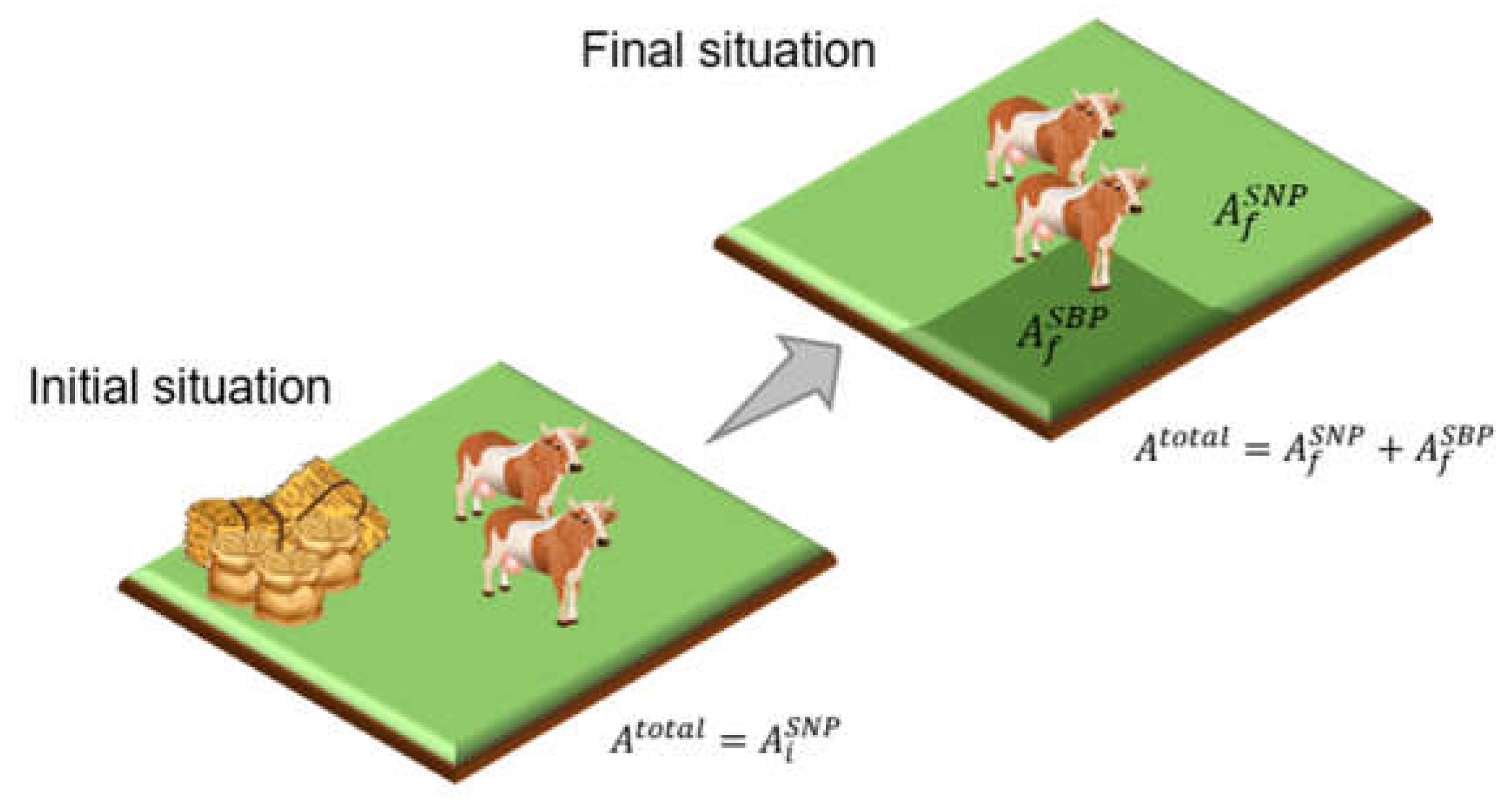
It would be inaccurate to directly compare the impacts of 1 ha of SBP to 1 ha of SNP due to the replacement of the concentrate. We thus considered two scenarios, which correspond to two instants commonly observed among farmers. In the beginning (“initial” scenario), farm land is used exclusively for grazing in SNP. SNP are mostly low-yielding grasses that fail to provide a complete feed. Ruminants in SNP require concentrate to complement their dietary requirements. At the second period (“final” scenario), farmers sow SBP, the high-yield mixtures of legumes and grasses that are more productive than SNP [10]. However, farmers will only sow the area required to suppress the need for commercial feeds, or the whole area of the farm, whichever is smallest. This is because of the fact that we assume livestock units (LU) are kept constant in the farm, and consequently there is no increase in total stocking rate [10]. Farmers do not need more area of SBP than what is strictly required for the stocking rate they possess, which remains constant throughout the analysis. This is depicted graphically in Figure 1. Please note that all abbreviations used in figures and tables are located at the end of the paper.
The functional unit (FU) is defined as 1 ha equivalent of SBP per year (equivalent because of the calculation of SBP area in the final situation as a function of the amount and nutritional quality of the commercial feed in the beginning; thus, the 1 ha equivalent of SBP comprises both SBP and SNP). The equivalence between scenarios is defined in Section 2.4.
2.3. Description of the System and System Boundaries
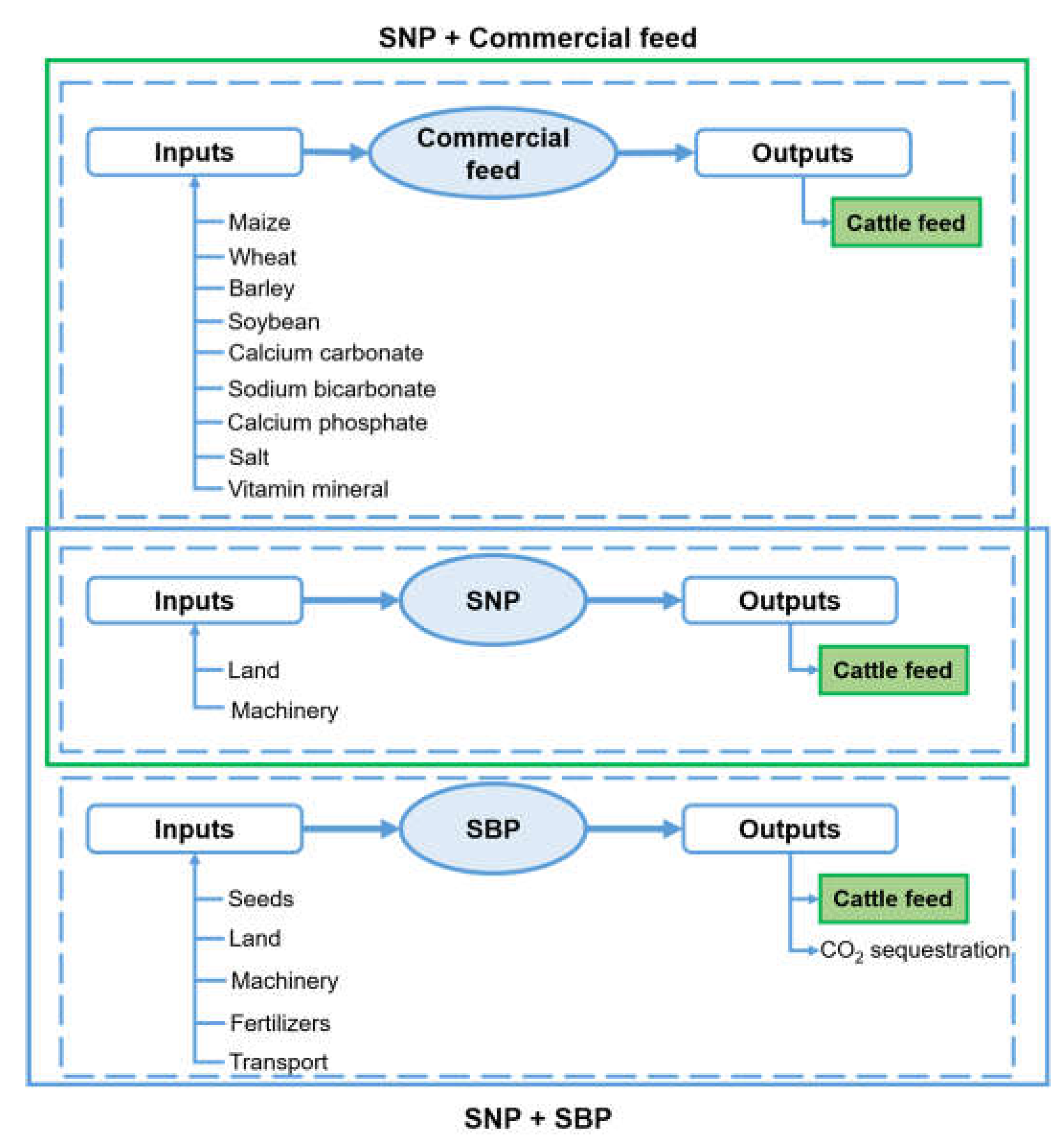
We included all cradle-to-farm-gate activities related to the three production systems involved in the two scenarios (Figure 2). Because of the use of CLCA as defined before, we include only the inputs and outputs that are exclusive to each of three production systems. The baseline system is a combination of SNP and commercial concentrate feed. The second system is a combination of SNP and SBP, using a representative seed mixture used by farmers in Alentejo from Teixeira et al. [10] for the latter. We assumed that, for each hectare in a farm, farmers replace a certain fraction of the hectare (previously occupied by SNP) with SBP until the need for concentrate feed is eliminated. SBP requires installation (year 1) and maintenance processes and intermediary consumption of materials.
There are, therefore, three subsystems (SNP pastures, SBP, and supplementary feed) within the two systems in the analysis (SNP + feed, and SNP + SBP). The SBP subsystem includes installation and maintenance activities and materials used (inputs), also including output flows associated (such as emissions). In the first year after installation of SBP, the pasture is not ready to be used as feed (in order to build the seed bank for re-sowing the following year). Concentrate is thus also required in the first year for the SBP system. The SNP system requires only machinery for field operations and associated emissions, as frequent tillage is necessary to remove invasive shrubs. The commercial feed system includes only the life cycle of the production of its ingredients. We assumed that the impacts of industrial concentrate manufacturing are negligible.
2.4. Scenario Equivalency
As described in Section 2.2, the condition for scenario equivalence is that the nutritional contents of concentrate are nutritionally fully replaced with the feed grazed in SBP. This condition must be operationalized in relation to particular nutritional indicators (e.g., energy, protein, or fiber), which for simplification, we generically designate as “nutritional forage units” (NFU). We followed the method proposed by Teixeira [9] to derive the equation for calculation of impacts, which follows from three balance conditions: (1) nutritional equivalence (the requirement that the total amount of a given nutritional indicator is equal in the initial and final situations); (2) area invariance; and (3) stocking rate invariance. This equivalence, together with the CLCA approach, means that all emissions that are invariant with the area or stocking rate were not included in the analysis as they are similar between scenarios. This included all emissions from animals (enteric fermentation, dung, and urine) and some emissions from soils (N2O emissions from soils). The Appendix of this paper provides a detailed description of the calculation procedure that leads to the establishment of the formula for the calculation of the difference of impacts between scenarios per functional unit. Note that throughout this paper, variables denoted in braces are per unit of area, and variables denoted in chevrons are per unit of mass. The difference of impacts for the first year is
where {I}ftotal is the total environmental impact in the final scenario, {I}itotal is the total environmental impact in the initial scenario, {I}SBP is the environmental impact per unit area of SBP, {I}SNP is the environmental impact per unit area of SNP, and AfSBP is the area of SBP installed. The criteria of area equivalence is not fully verified in this model because during the first year SBP, cannot be grazed, but the area of SNP has already been decreased—which could mean that farmers could need to provide additional feed to cattle unless they owned additional grazing land to momentarily compensate the decrease in SNP area. We assumed, as a simplification, the latter case, that is, that in the baseline situation, all area is covered by SNP, but for the first year in the final situation, the area of SNP is higher than the total area for the following years. {I}SBP and {I}SNP are determined using, respectively
and
where and are the CO2 equivalent impacts of the production and use of all inputs (machinery, materials, energy) used in management operations on SBP (installation or maintenance) and SNP, respectively; is the amount of nitrous oxide (N2O) emitted in SBP (measured in CO2 equivalents); and is the amount of carbon dioxide sequestered in SBP. These additional flows only exist in SBP and not in SNP, and as such, have to be considered in the difference between scenarios.
The difference in impacts between scenarios after the first year is calculated using
where ε is the ratio between the NFU provided by one hectare of SBP and that provided by one hectare of SNP, {NFU}SBP are the NFU of SBP per unit of area, 〈NFU〉feed is the NFU of commercial feed per unit of mass, and 〈I〉feed is the environmental impact of commercial feed.
We considered that the parameter ε is equal to the ratio between the average stocking rates of SBP (0.91 LU/ha) and SNP (0.39 LU/ha), which, using empirical data [28], is equal to 2.33. This difference in stocking rate is due to the difference in yield and quality of the pasture. Carneiro et al. [28] surveyed six farms over five years to discover that primary aboveground production is consistently approximately double in SBP in relation to that in SNP throughout the years of settlement. Additionally, SNP have few to no legumes, and consequently are lower in protein [29].
2.5. Inventory Analysis
In recent years, LCA regionalization has been one of the main trends within the LCA community [30], as it is of crucial importance for accuracy in results. There are now regionalized agricultural inventories in Portugal, and Alentejo in particular, that enable LCA analyses based on scale-consistent local data [31]. While in the past, the absence of data and models limited the analyses, there are now resources for using a specific inventory for SBP and SNP in Alentejo [31].
Regional fact sheets [32] from the Alentejo region in Portugal indicate that SNP require only an annual spring harrowing process. SBP installation involves materials (lime and fertilizers) and their respective transport and agricultural processes (sowing, liming, harrowing, rolling, and fertilizing) during the first year. After year 1, maintenance requires less agricultural processes (liming and fertilizing) and materials (Terraprima personal communication). We considered that SBP require the application of 2 t of lime for pH correction in installation and 0.4 t of superphosphate. Lime application then occurs every four years (year 4 and year 8 after installation) and superphosphate application every two years (years 3, 5, 7, and 9). This is a worst-case scenario, as in actual pastures, the need for liming and phosphorus is assessed through soil analysis and may not be required in the specified year. The inventory flows for these materials, as well as of the seed mix of grasses and legumes, were collected from the ecoinvent v3.4 database [33].
The ruminants used in the analysis were cows, namely the Alentejana breed, which is autochthonous and common in Alentejo. The composition of a typical commercial feed (concentrated and forage) for this breed is presented by Costa et al. [34]. The ingredients are maize, wheat, barley, soybean meal, sunflower meal, hydrogenated fat, calcium carbonate, and sodium bicarbonate. There are two main formulations of this feed, depending on the ratio of commercial concentrate/forage (low quantity of silage maize—LF; high maize silage content—HF) that is fed to the animals. Table 1 shows the amount of each ingredient in the feed. Inventory flows for these materials were also obtained from ecoinvent [33]. The full list of ecoinvent processes used are presented in Supplementary Materials File S1.
The idea of nutritional equivalence between SBP and commercial feed expressed by NFU in Equation (4) was operationalized using four nutritional indicators: crude protein (CP) (estimated nitrogen content of feed), crude fiber (CF) (indigestible carbohydrate component), neutral detergent fiber (NDF) (measures the structural components in plant cells), and gross energy (GE) (energy released by burning feed in excess oxygen). The values for each NFU in commercial feed are also shown in Table 1.
To determine which species are sown in SBP, we used a representative seed mixture from Teixeira et al. [10], reproduced in Table 2. Given that the exact amount of each species or variant in the mixture was impossible to obtain, we assumed that the distribution between legumes and grasses seeds is in the proportion of 60–40% [10]. We considered the number of grasses and seeds in the mixture and assumed equal distribution—that is, each legume species or variant was assumed to be 5% of the total and each grass was assumed to be 25% of the total. Nutritional indicators of each species/variant were obtained from INRA et al. [29] and are also presented in Table 2. When data for a specific species/variant were unavailable, we used a related variant from the same family. Namely, data for Trifolium repens were used to estimate data for Trifolium balansae; data for Trifolium incarnatum were used to replace Trifolium incarnatus; Trifolium alexandrinum data were used instead of those of Trifolium vesiculosum; and Ornithopus sativus data were used instead of those of Ornithopus compressus and Biserrula pelecinus.
In the absence of data, we assumed that animals only graze the species sown, and ignore spontaneous edible plants in SBP. Nevertheless, the abundance and proportion of total dry matter (DM) production of legumes–grasses is different from the proportion sown. Legumes and grass DM production varies along the years; in the first year, the proportion is 50/50%, but the fraction of legume yield decreases until approximately the fifth year and then remains constant, according to Teixeira et al. [10]. We assumed that legume abundance decreases 5% per year between years 2 and 5 (grasses increase at the same rate).
To estimate carbon dioxide sequestration in SBP, we used the calibration of the Rothamsted Carbon Model (RothC) by Morais et al. [35]. This model was calibrated specifically for SBP using measured data. The parameters used were the root to shoot ratio (0.98), livestock intake fraction (0.61), livestock excretion during grazing (1.53 t C/LU), and the RothC parameter of the ratio between easily decomposable plant material (DPM) and resistant plant material (RPM) (value: 1.09). We ran the RothC model using an aboveground productivity of 7 t DM/ha, stocking rate of 1 LU/ha, initial SOC content of 7.4 t C/ha (equivalent to the SOM concentration of 0.87% in 10 cm topsoil [11]), and the average climatic conditions in the region of Alentejo (temperature: 16 °C, precipitation: 75 mm [36]).
The N2O emissions from legume nitrogen fixation were calculated using firstly the nitrogen fixation factor for SBP in the Portuguese National Inventory Report (NIR) [37] of 0.026 kg N fixed/kg DM and a yield of 7 t DM/ha. Then, N2O emissions were calculated according to the Intergovernmental Panel on Climate Change (IPCC) emission factor (0.01 kg N2O–N kg−1 N fixed) [38].
The impact category selected in this study was global warming potential (GWP) for a time horizon of 100 years with climate carbon (CC) feedback factors (IPCC Fifth Assessment Report, AR5) [39]. The impact is expressed in kg of carbon dioxide equivalent (CO2e). The characterization factors for the most important GHG are 1 for CO2, 34 for CH4, and 298 for N2O. Impact assessment was carried out up to the classification and characterization phases. Normalization and weighting were not performed so that results could be interpreted independently at midpoint. We used the SimaPro 8.5 software to perform the impact assessment.
2.6. Scenario Assessment
Equation (4) provide the difference in impacts between scenarios on a hectare of SBP basis. It does not require knowing the exact fraction of the farm that is occupied by SBP in the final scenario. The fraction of farm that is sown, that is, how much area of SBP farmers have to install in order to eliminate concentrated feeds, is co-determined with the amount of feed provided to animals. Maintaining the notation of the Appendix, let denote the fraction of the area in the final scenario that is occupied by SBP, and let denote the weight of concentrate/silage fed to animals per hectare in the initial scenario. It can be shown (in the Appendix A) that neither one can be determined independently, that is, there are several combinations of the two variables that yield the same environmental impacts. The relation between the variables is expressed by
The terms on the right-hand side of the equation are known, as shown previously. Parameter ε is 2.33, and the others are obtained from Table 1 and Table 2. For each possible value of (which varies between 0 and 1), we calculated the quantity of concentrate provided to the animal, in the absence of SBP.
Then, to check if scenarios are indeed equivalent, we multiplied the amount of concentrate by to obtain the total nutrition provided by the concentrate. We summed the latter value to (which we know is approximately half of the value for SBP, because ε = 2.33) to obtain the total nutrition provided to animals in the initial situation. Then, we determined the nutritional amount of feed provided in second scenario, which is equal to the sum of the product of the fraction of SBP and and the fraction of SNP (which is 1 − x) multiplied by .
One last verification was made by using the most likely for this breed of Alentejana cows, and then checking whether the respective value for x is similar to the observed fraction of the area sown in farms in the PCF project. In this project, farmers on average sowed up to 20% of the areas of their farms (Terraprima, personal communication). We calculated as the product of the following: (a) the stocking rate of 0.39 LU/ha [28], considering that there is always one adult cow and one steer together in the pasture (one birth per year, and the steer is sold at one year old), where one adult cow is 1 LU and one steer is 0.4 LU; (b) the weight of the one-year-old steer (323.7 kg) [40] and the adult cow (677.3 kg); and (c) the amount of feed one cow and steer eat per day, which is between 0.5% and 1.5% of their live weight. Using these estimates for , we applied Equation (5) to obtain a lower and upper bound for the SBP fraction (), and , respectively. We also considered an average feed consumption () for animal intake of 1% of live weight. With , , and values, we calculated the lower, upper, and average of the impact, respectively, in each individual scenario (SNP and commercial feed) as well as SBP and SNP (using Equations (A5) and (A7) in the Appendix A, respectively). We also assessed εcrit, the value required for the difference in nutritional quality between pasture types such that all area would have been converted to SBP—defined by x = 1, using Equation (A18), for each x value. Finally, we estimate the difference between situations according using, for the first and following years, respectively,
and
This procedure, expressed by Equations (6) and (7), enables the calculation of the difference of impacts per unit of area of the farm, rather than area of SBP. We then also changed the reference unit from area to meat produced to obtain the difference in impacts between scenarios for each kg of meat. This analysis assumed that the carcass output of each one-year old steer is equal to 70.1% of the live weight of the animals [40]. We thus assessed the potential reduction of the total impacts of beef production due to conversion to SBP, considering a similar production system, from Eldesouky et al. [41], which studied an extensive production system in the Spanish Montado (considering the “extensive beef/calf cattle farm” production system, with calves sold at weaning). The commercial feed consumed was mostly composed by forage, similar to the HF feed considered in this study (percentage of forage: 74% for Eldesouky et al. [41] and 70% in this study). The stocking rate in this study was also similar to the SNP stocking rate (Eldesouky et al. [41]: 0.36; SNP in this study: 0.39). We also assessed avoided emissions considering the global average beef production impacts, from Poore and Nemecek [42].
3. Results
3.1. Nutritional Equivalencies between Pasture and Concentrate
Table 3 displays the average nutritional equivalence ratio, along the years, between SBP and commercial feeds (LF and HF). The ratio in LF feed is always higher than that in HF feed. The ratio for CF is the highest for HF feed type because SBP plants have more CF than maize silage (which is 70% of the overall feed). Regarding the LF feed, the ratio for NDF is the highest, as it is also related to the fiber content of plants. The indicator related to energy (GE) is where the ratios are lower, meaning that the concentrate provides comparatively more energy than nutrients to cattle. The nutritional equivalence ratios tend to increase with time because of the reduction of legumes and increase of grasses (with higher nutritional index values). The variation between ratios is higher in the LF feed than in the HF feed. The HF ratios are mostly dominated by the maize forage (70% of total mass), while in the LF feed, the proportion is more diluted among all ingredients, which leads to more variance in nutritional values. The ratios in Table 3 enabled the environmental impact assessment using Equation (4).
3.2. Life Cycle Impact Assessment
The vast majority of the impacts of SBP (installation and maintenance) are because of lime and phosphorus fertilizer production, transportation, and application. In the installation of SBP, lime application is responsible for 61% of the total impact. In the following year, phosphorus fertilizer is responsible for 80% (in years without lime application). Regarding the feed, soybean meal is the main source of impact, in both formulations, with 45% (in the LF feed) and 37% (in the HF feed). Soybean meal only represents 10% (LF feed) and 5% (HF feed) of the feeds, but its unit impact, 4.4 kg CO2e/kg, is significantly higher than cereals grains (e.g., maize grain: 0.63 kg CO2e/kg) and maize silage (0.16 kg CO2e/kg) because of the difference in the cereals productivity (higher maize silage productivity dilutes the impact in a higher quantity of product than the maize grain with lower productivity). The LF feed impact is 0.92 t CO2e/t feed; for the HF feed, the impact is 0.49 t CO2e/t feed. Regarding carbon sequestration, it is higher in the first year (12 t CO2/ha) and decreases during the 10-year period (in the tenth year carbon sequestration is about 2 CO2/ha), until soil organic matter (SOM) saturation is eventually reached. N2O emissions from legumes are 1 t CO2e/ha in the first year and then decrease, reaching 0.825 t CO2e/ha in the fifth year.
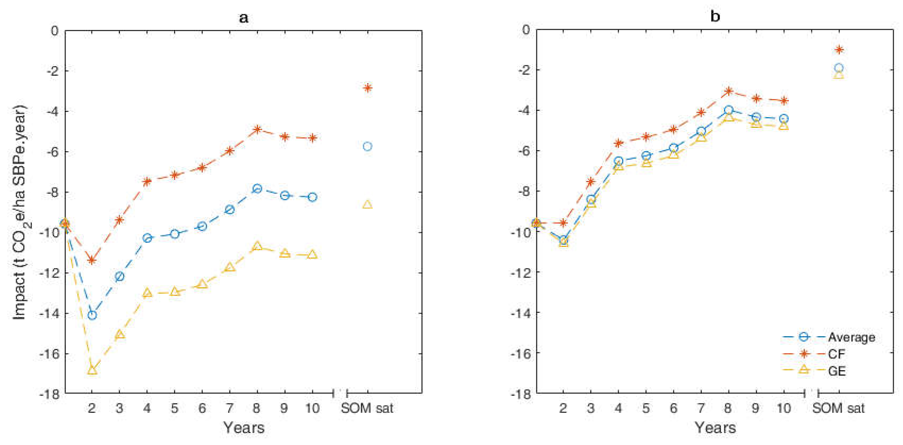
The full list of results is available in Supplementary Materials File S1. Figure 3 depicts the difference between the final situation (SNP and SBP) and the initial situation (SNP and commercial feed). In Figure 3, a negative value means that in final situation, the impact is lower than in the baseline situation. In the scenario with SBP and SNP, GHG emissions are lower than in the baseline situation in every year, including the first year (SBP installation year). Despite the fact that in the first year, there is no usable yield, the carbon sequestration more than compensates for feed requirements. Figure 3 also shows, for the nutritional indicators used to establish scenario equivalency, the average, minimum (GE), and maximum (LF feed: CF; HF feed: NDF) results. Replacing LF feed (Figure 3a) saves more GHG emissions than replacing HF feed (Figure 3b) on average. The impact difference reduces significantly in the second year because there are no inputs in SBP (including liming) and carbon sequestration is still high (8.5 t CO2e/ha). In the third and fourth year, the impact difference reduces significantly because of phosphorus fertilizer (in third year) and liming (in the fourth year) and carbon sequestration reduces to 3 t CO2e/ha.
The only aspect that significantly influences differences in results is the nutritional indicator used to establish an equivalence between scenarios. This is particularly important because commercial feeds, on a nutritional unit basis, have much higher impacts than SBP and SNP (e.g., LF feed: 6.5 t CO2e/t CP; HF feed: 3.5 t CO2e/t CP; SBP: 0.5 t CO2e/t CP). The variation between GE and CF in LF feed is 5.7 t CO2e/ha SBP, while in HF, it is only 1.3 t CO2e/ha SBP. This occurs as a result of lower variation in the nutritional ratios (Table 3) of the HF feed because of the high proportion of maize silage. On average, LF feed substitution leads to an avoided impact that is 60% higher when compared with the avoided impact using the HF feed.
The difference of impacts between scenarios diminishes SOM saturation (“SOM sat” in Figure 3) is reached, that is, when SBP no longer significantly store carbon in soils. The impact differential from this year on can only be attributed to the reduction in emissions due to the replacement of concentrate with SBP. The long-term effect of SBP is thus a saving of between 2 and 6 t CO2e per hectare of SBP and per year.
3.3. Scenario Assessment Results
The full list of results for the scenario assessment is available in Supplementary Materials File S1. Table 4 shows the co-dependency of and x, resulting from the application of Equation (5) for specific numbers of x. The higher the quantity of feed that is given to animals in each hectare of SNP in the initial situation, the greater the area of SBP necessary to replace it. As we considered a constant nutritional provision by each type of pasture, this also means that more energy is required by cattle. The quotient between and varies between the first and fifth year (due to the change in prevalence of legumes) and is on average 3.8 kg LF feed per ha of SBP and 3.1 kg HF feed per ha of SBP. The same area of SBP installed thus replaces a lower amount of HF feed than of LF feed. Regarding and (or ), they are equal for both feeds, according to Equations (A3) and (A4), respectively. As all the parameters in Table 4 are explicitly dependent on (SBP fraction), they increase when also increases.
We obtained an average of 13% (LF feed) and 14% (HF feed) considering that one cow and steer eat 0.76 t/ha·yr per day. The for the LF feed ranges between 7% and 20%, and between 10% and 21% for the HF feed. The maximum in both feeds is obtained using GE equivalence. GE is similar in both commercial feed formulations (Table 3). The was calculated considering that one cow and steer eats 0.5% of its live weight (0.39 t/ha·yr) per day. The average is 6% (LF feed) and 7% (HF feed). The ranges between 4% and 10% (LF feed) and between 5% and 10% (HF feed). The was calculated considering that one cow and steer eats 1.5% of its live weight (1.14 t/ha·yr) per day. The average is 19% (LF feed) and 21% (HF feed). The ranges between 12 and 30% for both feed types. These results for mean that SBP would never need to be installed in more than a third of the farm area to compensate for a realistic amount of concentrate consumption—and usually are installed in 20% or less of the farm. This is because of the relatively high nutritional content of SBP plants when compared with concentrate feed ingredients.
For each value of , there is a (which corresponds to converting 1 ha of SNP in SBP). The does not change considerably between years (nutritional ratios are similar between years) and between feed types. For the , the average f is 1.17 or LF feed and 1.18 for HF feed. For the , the average is 1.08 (LF feed) and 1.09 (HF feed). Finally, for the , the average is 1.25 (LF feed) and 1.27 (HF feed). Consequently, SBP only need to be marginally more productive than SNP for the replacement to pay off.
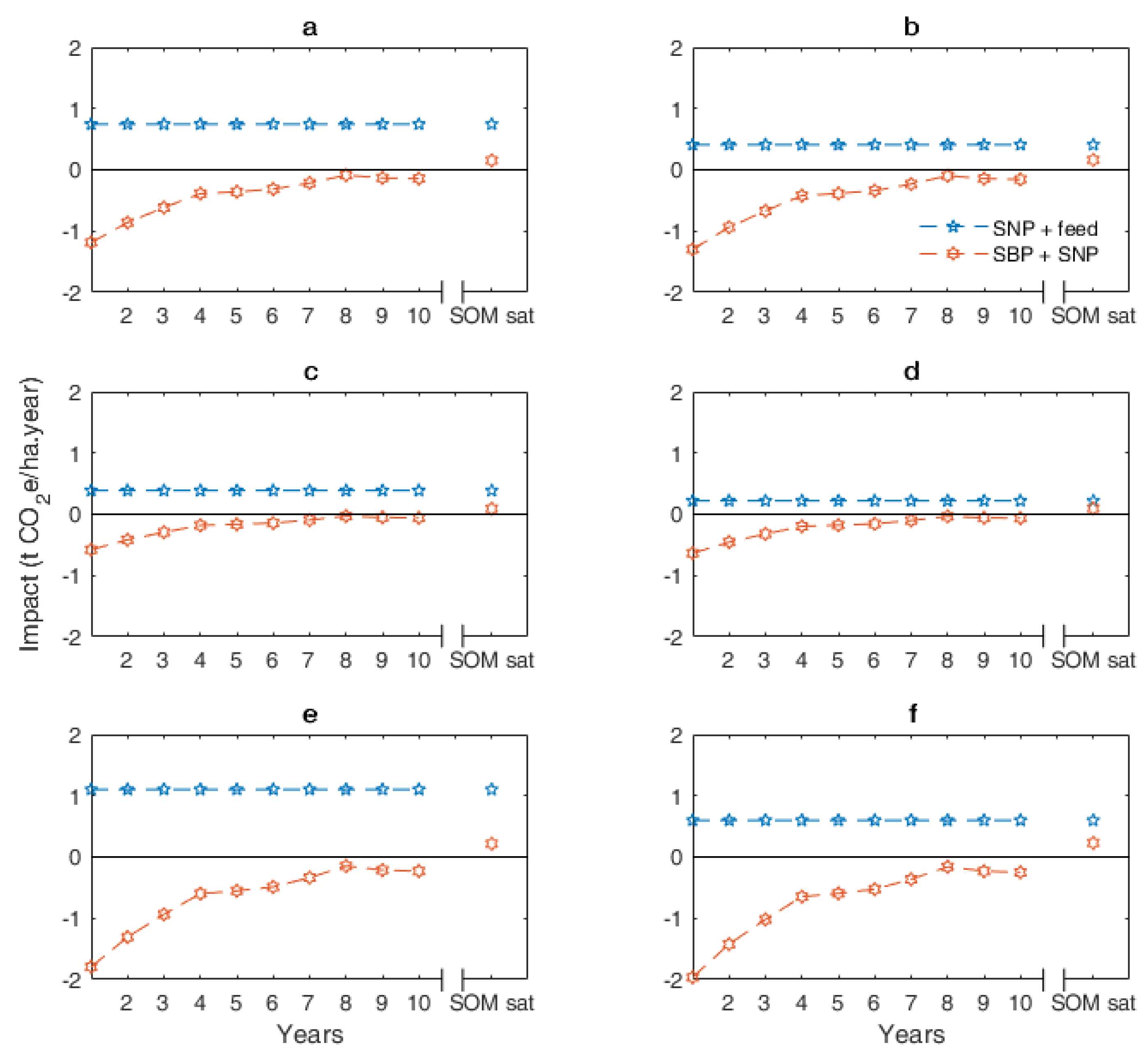
Figure 4 depicts the impacts of each scenario individually (rather than the difference between the two). The initial situation (SNP and feed) is shown in blue and the final situation (SBP and SNP) in orange. Regardless of , the impact in the initial situation is always greater than zero, mainly because of feed consumption (the only operation used in SNP is one annual tillage). Regarding the feed, HF feed leads to a lower impact, because its unitary impact is significantly lower than for LF feed. The impact of the final situation during the first 10 years is always negative as a result of carbon sequestration (a similar trend as shown in Figure 3). When SBP no longer sequestrate carbon (i.e., reach SOM saturation), the impact of the final situation is higher than zero because of the annual tillage operation in the SNP fraction of area (i.e., 1 − ). In the 10-year period, impact increases with the reduction of , as carbon sequestration is lower ( leads to lower impact avoided; and leads to higher impact avoided). When SOM saturation is reached, the greater the , the greater the impact, because the area where N2O emission occurs is higher (average impact of for HF feed: 95 kg CO2e/ha plot (SBP + SNP); average impact of for HF feed: 229 kg CO2e/ha plot).
The difference in impact between scenarios per unit of farm area when SBP no longer sequester carbon, calculated using Equation (7), is shown in Table 5. The results per kg of meat produced are also present in Table 5. As in Figure 3, a negative number means that the final scenario (SBP and SNP) has lower emissions than the baseline (SNP and feed). Regardless of the year, the difference of impact between the two scenarios is negative, even when SBP reaches SOM saturation. This is because of the effect of feed substitution dominating over the extra emissions from material and energy use in SBP. The impact avoided is 591 (LF feed) and 247 kg CO2e/ha (HF feed), considering the . The impact difference also increases with the SBP area as a result of the increase of with . The avoided impact per kg of meat is 17 (LF feed) and 7 kg CO2e/kg meat (HF feed), considering the . In the initial 10-year period after SBP installation, avoided impact is even higher, 35 (LF feed) and 26 kg CO2e/kg meat per year (HF feed), for .
For a similar production system in Spain [41], the meat production impact obtained was about 21 kg CO2e/kg beef live weight, converting from IPCC AR4 GWP factors [43] to IPCC AR5 [39] (30 kg CO2e/kg of fat- and bone-free meat, considering the carcass output is equal to 70.1% of the live weight of the animals [40]). Thus, SBP installation could reduce total impacts of beef by about 25% (using HF feed avoided impact from Table 5, for ). The world average meat production impact is 90 kg CO2e/kg of fat- and bone-free meat [42] (using IPCC factors with CC feedbacks [39]). This value includes different production systems, also including purely intensive production, and as such, it is not comparable with results from this study. Nevertheless, if we assume that the Spanish production system is on the lower end of the distribution of global average impacts, simply using the SNP + HF feed would already reduce emissions from approximately 90 to 21 kg CO2e/kg beef live weight. There would be an additional 25% reduction from further converting to SBP—leading to a potential total accumulated reduction of average emissions due to the production of meat in the SNP + SBP scenario of approximately 80%.
4. Discussion
The results of this paper assess and compare the environmental impacts of two realistic pasture systems in Portugal as a way to assess the consequential effects of installing and maintaining SBP. The comparison was performed using an innovative approach that resorts to energy and nutritional equivalences between the systems first proposed for the specific comparison of pasture systems by Teixeira [9]. The analysis was greatly simplified because of the fact that there is ample empirical evidence that one scenario does follow from the other one. In the 1000 farms of the PCF project, SBP were installed in former areas of SNP. Therefore, rather than performing a dedicated LCA for each system, which would be more burdensome and include redundant processes and flows, we followed a simpler and easier to interpret comparative approach. The consequential approach followed is interesting in this case because SBP cannot be assessed without including effects that are inextricably connected with their installation and added material and energy consumption, as well as feed avoided. So far, however, this analysis had stayed at the farm level and included only direct emissions. The approach followed here highlights these effects rather than diluting them within the entire carbon footprint of meat products for each of the systems.
The results show that phosphorus fertilizer and lime application are the main contribution to the total emissions assessed for SBP pastures (for installation, but also for maintenance). This issue was identified in Teixeira et al. [10], but never duly quantified. Phosphorus fertilizer is not only an environmental issue in SBP, but also an economic issue, as identified by Almeida et al. [44], as the fertilizer costs have been gradually increasing over the years. As future work, an economic comparison between systems should be made in order to complete the assessment. For example, through life cycle costing (LCC), as suggested by several authors [45,46,47], with the purpose of emphasizing relationships and trade-offs between the economic and life cycle environmental performance.
Regarding the equivalence method, it is possible to conclude that energetic equivalence provides different emissions in comparison with crude protein and fiber equivalences. For example, when crude fiber is used to establish the equivalence of scenarios, the difference between scenarios is about 50% higher (low forage feed) than when using gross energy. This is because of the fact that SBP have higher nutritional quality and thus can replace more quantity of feed. For high forage feed, the variation between nutritional equivalences is significantly lower as silage dominates the composition of the feed and the variability of the indicators is smaller.
To assess the variability of the results when faced with different assumptions, we used sensitivity analysis whenever possible. One example is the required feed consumption for the desired growth level of the steer. This analysis revealed high sensitivity of results depending on the animal feed requirements considered (0.5% or 1.5% of live weight). The difference between scenarios increases with higher feed requirements because of the high unitary impacts of the concentrate.
There were, however, several assumptions made in the work that influence results and we were unable to include them in the (quantitative) sensitivity analysis. Reverting some of these assumptions would likely cause the difference in emissions between the scenarios to increase, while for others, it would decrease. Starting with assumptions that would make the relative benefit of sowing SBP larger, there is the fact that it is not entirely true that SBP cannot be grazed during the first year. Although it is a good management practice to avoid grazing during the establishment of the pasture to ensure a good seed bank for the following years, during the summer months, it is possible (and desirable) to graze in order to ensure good germination of grasses and legumes during autumn, as well as to control infesting plants. This means that animals do take some of their feed from SBP during the first year, and consequently there is some replacement of concentrate. This fact would improve the performance of the system with SBP. Additionally, relatively to commercial feeds, we assumed that all ingredients were produced locally (in the farm where the pastures are situated). This is a conservative approach that underestimates the impacts of feeds, mostly because it disregards feed transport, which can be an important phase because of consumption of energy and associated GHG emissions (can contribute up to 15% of total emissions of the feed) [5,42]. This approach could only amplify the differences between systems, as considering more transportation of ingredients would make the unitary impacts of the feed larger. These assumptions do not compromise the main conclusions regarding the comparison of scenarios.
Regarding assumptions that would lower the difference between scenarios, the most important one is that we did not consider any feed consumption in SBP. This was a simplification required because of the lack of data on the distribution of DM yield in SBP throughout the year. Good practices for SBP management state that at least during early spring, grazing should be light to ensure a healthy re-establishment of the seed bank. It is also possible that during the summer months, yields decrease as a result of the lack of rainfall—as these are rainfed pastures. If we assume a worst case scenario where there is no pasture intake during one month in early spring and two months in the summer, that would mean that for one quarter of the year, cattle would require feed. This means that all results presented here would be approximately reduced by one quarter. For example, the avoided impact per kg of meat would be approximately 13 (rather than 17) for LF feed and 5 (rather than 7) kg CO2e/kg meat for HF feed. This would also not compromise the main conclusions from this study. Also relevant to note is that SBP are technically more demanding from farmers and their installation can fail. A critical problem is the lack of prevalence of legumes. However, the sample of farms used to collect data used in this assessment [28] included some cases where the installation was less than fully successful. Therefore, the assessment in this work was already carried out using an average of all likely situations. Finally, we used two realistic feed formulations that enabled us to test the effects of silage, but there is a vast array of feeds used for beef cattle in Portugal. Feed formulations can and should also be optimized to achieve specific animal growth requirements and to better complement nutrition obtained from pastures, as well as to decrease GHG emissions [48]. In this paper, we did not assess those potentially optimized feeds. We also used a commercial feed formulation rich in cereal grains. Some commercial feeds include a higher share of co-products (cereals husk, meals, and others). Those feeds can have lower impacts [49], depending on the exact co-products. Here, we additionally considered that changing animals diets would not change live weight gain, which is a simplification that can change the results for avoided impact per kg of meat. Further, the feeds used were originally intended for fattening, and not for less than one-year-old steers or adult cows. Given the high energy provided by the feed to the animal, the fact that we consider this particular feed here means that the difference between scenarios could even be larger (as less area of SBP might be needed to replace feeds). In the future, results can be improved by considering the change in live weight gain due to changes in diets and the different commercial feeds consumed by different animal classes.
Other assumptions made are more unclear regarding the consequences for results. We assumed that ε = 2.33, which is equal to the ratio between stocking rates in SBP and SNP, according to Carneiro et al. [28]. The definition of this parameter is a ratio between nutritional contents, but the lack of a representative breakdown of the species composition of SNP prevented us from using that definition literally. Therefore, we used stocking rates as a proxy. We also assumed, in the calculation of nutritional equivalencies between scenarios, that the proportion of the area of SBP was equal to the proportion between dry matter.
Here, we also used the IPCC AR5 GWP factors with CC feedback for impact assessment. The GWP factors with CC feedback are higher than the factors without carbon feedback (e.g., N2O with CC factor: 298; N2O without CC factor: 265). Nevertheless, the results are not considerably affected by this. If IPCC GWP without CC feedbacks had been used, the savings due to conversion to SBP would decrease by less than 6% (i.e., less than 0.1 t CO2e/ha). Finally, we did not consider N2O emissions from pastures litter. We assumed that the litter fraction is equal in both situations (SNP plus commercial feed and SBP plus SNP).
Future developments to this paper should be considered in the future. One example is the reassessment of the N2O emissions from legumes. Here, we used a default value to estimate this flux. However, the factor was not dependent on the fraction of legumes (responsible for soil nitrogen fixation and soil N2O emissions). Further, the IPCC [38] does not even consider N2O emissions from biological nitrogen fixation because of a lack of evidence that they contribute significantly to soil N2O emissions. If we had disregarded those emissions, the avoided impact due to SBP installation would be even higher. Finally, an option to improve the estimation of livestock intake and animal growth may be the use of mass-balance approaches [16].
Ultimately, we converted our reference flow into a mass unit (kilograms of meat as a final product) as it is the choice of most studies targeting meat production (among others, [41,50,51,52]). Alternatively, another common unit in other studies is one live animal (among others, [53,54]). This mass unit should, however, be adjusted for nutritional value, as performed by Poore and Nemecek [42]. Meat from SBP and meat produced using concentrate feed likely diverge in terms of their quality, as meat from SBP is nutritionally superior [10], as well as carcass yield, so new differences may arise if this differentiation is included in future LCAs of these systems.
Species variability in SBP is the most relevant uncertainty not addressed in this paper. Further improvements in the estimation of carbon sequestration can also be made, namely through the application of a geographical LCA, where the difference between scenarios is assessed for multiple sub-regions within Alentejo. The key parameter missing to perform such an evaluation is a regionalized estimation of the yield of SBP. A remote sensing approach is a viable alternative to estimate regionalized aboveground biomass productivity [55,56]. This approach also has limitations, such as, for example, the influence of tree cover. This effect is particularly relevant in these “Montado” agri-forestry regions due to high tree cover density (e.g., 170 trees/ha of Quercus suber [57]), 2 as trees also influence aboveground biomass productivity [58]. Here, we used the process-based model RothC calibrated for SBP (root to shoot ratio, livestock intake fraction, livestock excretion during grazing, and easily decomposable plant material (DPM)/resistant plant material (RPM) ratio), which can consider some site-specific conditions if available—such as regionalized aboveground productivity and stocking rate. Regionalization would be welcome for other parameters of the study. For example, we used a single mixture of sown species, but mixtures are tailor-made for different site conditions (such as soil density and soil organic matter (SOM)). Even more importantly, the species found in the pasture some years after installation could deviate considerably from their proportion in the mixture of seeds used. This could considerably change the nutritional value of the pasture. For example, in the same group, average CP content in two distinguished clover species can range from 19% DM (for Trifolium subterraneum) and 25% DM (for Trifolium balansae). This difference can be even more significant between different plant groups [29]. Further work is required to better understand species variation with location, management practices, and other aspects not identified yet. To do this, more field work is required, including multiple sites studied over a long period.
In this study, we only focused on the contribution of SBP for climate change mitigation. Nevertheless, in the future, other ecosystem services should be addressed, for example, leaching reduction or effects on biodiversity [59]. There is evidence that SBP reduce nitrogen leaching when compared with SNP [60], but not in a life cycle assessment approach. Besides placing more emphasis on the regionalization of the inventories and activity data, these additional impact categories should also be assessed using regionalized life cycle impact assessment methods [31]. There are now multiple highly regionalized methods available, mainly focusing on land use [61,62] and biodiversity impacts [63,64].
5. Conclusions
Through the comparative assessment of GHG emissions of two cattle feed systems in Alentejo, Portugal, we found that the system with a combination of SNP and SBP has lower emissions than the system with SNP and feed, for both feeds considered. The main reason for this is that the replacement of concentrate by SBP is highly beneficial in terms of GHG emissions. The main protein sources of the concentrate, such as soybean meal, have high unitary impacts, and as such, even a minimal level of replacement with SBP grazing can compensate for the added impacts due to fertilization and liming. SBP have the added benefit of sequestering carbon (on average, 8 t CO2e per hectare of SBP and per year during the 10-year period after installation), but the beneficial effects of replacing feeds take place even after SOM saturates in SBP soils. The installation of SBP in less than 20% of the area of SNP can thus avoid 3 t CO2e per hectare of SBP and per year simply because of the replacement of the feed. Per kg of meat, this decreases emissions by at least 25%, considering comparable grazing systems.
Supplementary Materials
The following are available online at https://www.mdpi.com/2071-1050/10/11/4184/s1, S1: Ecoinvent processes used and results.
Author Contributions
R.F.M.T. conceived and wrote the bulk of the text. T.G.M. collected and managed data and carried out most of the calculations. T.D. co-conceived and supervised the study, and assisted in the writing process.
Funding
This work was supported by FCT/MCTES (PIDDAC) through project UID/EEA/50009/2013 and by project Animal-Future—Steering Animal Production Systems Towards Sustainable Future, funded by the Horizon 2020 Program of the European Union (SusAn/0001/2016). T. Morais was supported by grant SFRH/BD/115407/2016 from Fundação para a Ciência e Tecnologia and by FCT/MCTES (PIDDAC) through project UID/EEA/50009/2013.
Conflicts of Interest
The authors declare no conflict of interest.
Abbreviations
The following abbreviations are used in this manuscript, including variable names (with variable units in parentheses):
| CC | Climate carbon |
| CF | Crude Fiber |
| CLCA | Comparative life cycle assessment |
| CH4 | Methane |
| CO2 | Carbon dioxide |
| CO2e | Carbon dioxide equivalent |
| CP | Crude Protein |
| DM | Dry matter |
| DPM | Easily decomposable plant material |
| FU | Fucntional unit |
| GE | Gross energy |
| GHG | Greenhouse gas |
| GWP | Global warming potential |
| HF | High forage |
| IPCC | Intergovernmental Panel on Climate Change |
| LCA | Life Cycle Assessment |
| LCC | Life cycle costing |
| LF | Low forage |
| LU | Livestcok unit |
| NDF | Neutral detergent fiber |
| NFU | Nutritional forage units |
| NIR | National Inventory Report |
| N2O | Nitrous oxide |
| PCF | Portuguese Carbon Fund |
| RothC | Rothamsted Carbon Model |
| RPM | Resistant plant material |
| SBP | Sown biodiverse permanent pastures rich in legumes |
| SNP | Semi-natural pastures |
| SOM | Soil organic matter |
| Sown biodiverse permanent pastures rich in legumes fraction |
Appendix A
To define the equivalence between scenarios, we begin by defining several balances. We follow the method proposed by Teixeira [9]. Variables presented as <> express quantity of per unit mass, and {} express quantity of per unit area. All variables were defined on an annual basis (omitted for simplicity).
The first equivalence is the area balance, measured in hectares (ha), which states that the total area () must be equal to the SNP area () in the beginning (time i), and to the sum of the areas of SNP () with SBP () in the second scenario (time f).
Next is the livestock balance. The stocking rate is measured in livestock units per unit area (), a unit that measures livestock heads on the basis of the nutritional or feed requirement of each type of animal. The number of LU is constant in the two scenarios (no change in animal stock).
As there is no change in stocking rate, the animal feed energy requirements in the two scenarios are the same, which leads us to the energy balance,
where we have introduced the nutritional forage units measured in nutritional indicator per unit area (ha) of the commercial feed and the feed grazed on pastures by the cattle (), respectively. Note that these may be more than strictly required at time i and/or f. However, providing more NFU (e.g., energy, protein, fiber) than required to animals would be cost-ineffective to farmers, and as such, we use as an assumption exact nutritional equivalence between scenarios. Regarding the feed, the energy content is assessed per unit of mass. In order to do so, a conversion is required
where is the quantity of feed (t) required yearly per area unit of SNP in the initial scenario.
Regarding the impact calculation, in the initial scenario, the impact is the sum of the impact of SNP and the feed in the entire area of the farm.
where is the environmental impact per hectare. The commercial feed impact should be assessed per unit of mass, and as such,
The impacts in the second scenario are
where and are
where and are the environmental impact of management operations on SBP (installation or maintenance) and SNP, respectively. is the amount of nitrous oxide (N2O) emitted in SBP, and is the amount of carbon dioxide sequestered in SBP.
Therefore, the difference in impacts between the two scenarios is as follows:
Rearranging the expression using the area balance in Equation (A1) and substituting from Equation (A6), we find the following:
As our objective is to find the impact of the installation of 1 ha of SBP (which is the functional unit), we should divide Equation (A11) by the area of SBP.
Two terms in Equation (A12) are unknown: (we do not know how much feed is consumed per hectare of SNP because there is large variability and uncertainty due to farm-specific variations); the fraction of total farm area that is sown with SBP (area required to replace commercial feed). We define this fraction as (dimensionless).
We then return to the energy balance Equation (A3) and use the area balance and to modify it.
Dividing this equation by ,
Here, we need to introduce a new variable, the ratio of forage production between SBP and SNP ().
We define this variable because the energy content per unit area of both pasture types is unknown. However, we know that it should be roughly proportional to the ratio between stocking rates in SBP and SNP. Therefore, we may assume that the ratio in stocking rates (dimensionless) corresponds to the ratio in forage content of both types of pasture.
Using this variable in Equation (A15), and solving for x, we obtain
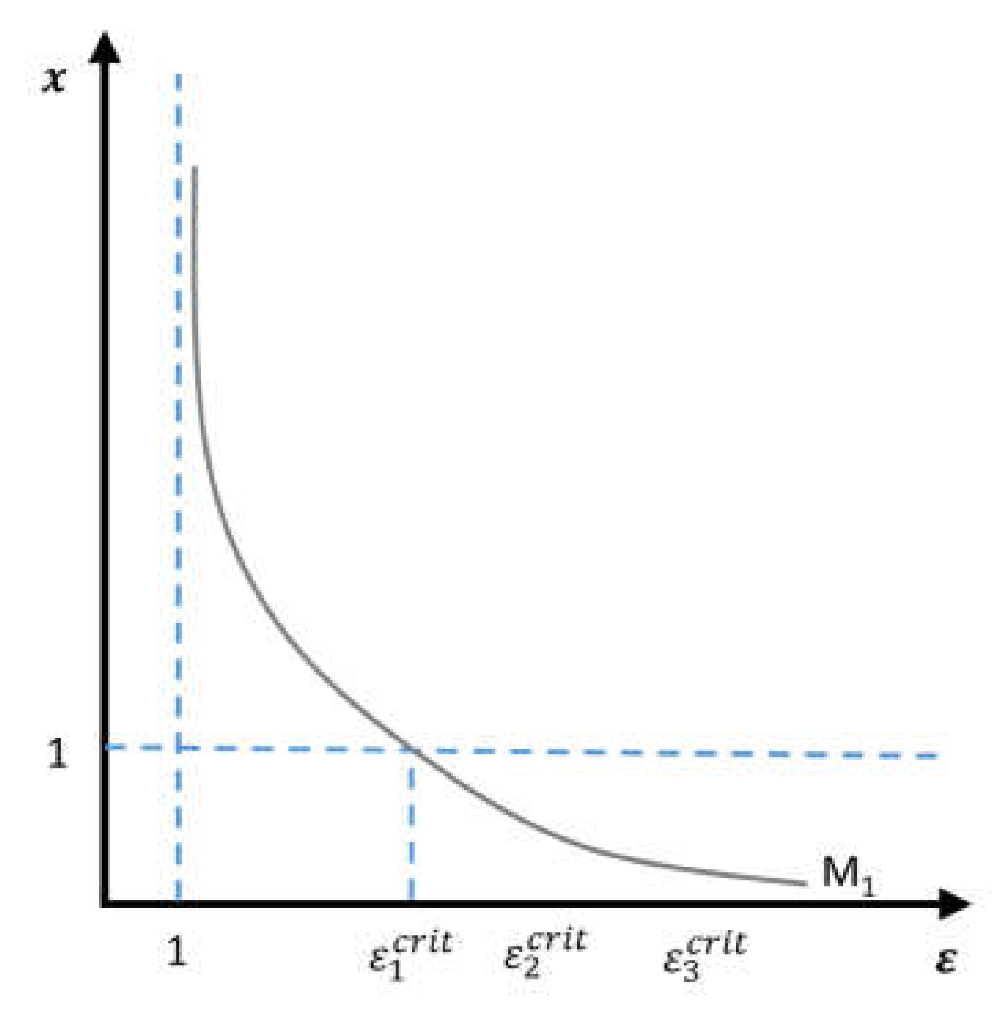
The graphical representation of Equation (A17) is shown in Figure A1.
Figure A1.
Effect of the nutritional quality of SBP (ε) on the fraction of the farm sown with SBP (x).
Figure A1.
Effect of the nutritional quality of SBP (ε) on the fraction of the farm sown with SBP (x).

There is an εcrit, which is the value for which all area is converted to SBP—and thus is defined by x = 1. Resorting to Equations (A15) and (A18),
We return to the difference in impacts between scenarios per unit of SBP area. We use the inverse of Equation (A16) and substitute it in Equation (A17) to obtain
Finally, using ,
In the first year, SBP are unusable as feed, so there is no replacement of concentrate. Equation (A20) simply becomes
We assume that ε is equal to 2.33, as the ratio between average stocking rate of SBP (0.91 LU/ha) and SNP (0.39 LU/ha), from empirical data [28]. These equations can be converted to express the average impact in the total area. For that, they must be multiplied by x (Equation (A13)), in Equation (A20), but using the prior equivalent version of the final term on the right-hand side in Equation (A20), this results in
The term can be replaced using Equation (A17).
Simplifying
Conversely, for the first year,
References
- Smith, P.; Martino, D.; Cai, Z.; Gwary, D.; Janzen, H.; Kumar, P.; McCarl, B.; Ogle, S.; O’Mara, F.; Rice, C.; et al. Greenhouse gas mitigation in agriculture. Philos. Trans. R. Soc. Lond. B Biol. Sci. 2008, 363, 789–813. [Google Scholar] [CrossRef] [PubMed] [Green Version]
- Leip, A.; Weiss, F.; Wassenaar, T.; Perez, I.; Fellmann, T.; Loudjani, P.; Tubiello, F.; Grandgirard, D.; Monni, S.; Biala, K. Evaluation of the Livestock Sector’s Contribution to the EU Greenhouse Gas Emissions (GGELS)—Final Report; European Commission, Joint Research Centre: Ispra, Italy, 2010. [Google Scholar]
- Garnett, T. Livestock-related greenhouse gas emissions: Impacts and options for policy makers. Environ. Sci. Policy 2009, 12, 491–503. [Google Scholar] [CrossRef]
- Steinfeld, H.; Gerber, P.; Wassenaar, T.; Castel, V.; Rosales, M.; de Haan, C. Livestock’s Long Shadow: Environmental Issues and Options; Food and Agriculture Organization of the United Nations (FAO): Rome, Italy, 2006. [Google Scholar]
- Roy, P.; Nei, D.; Orikasa, T.; Xu, Q.; Okadome, H.; Nakamura, N.; Shiina, T. A review of life cycle assessment (LCA) on some food products. J. Food Eng. 2009, 90, 1–10. [Google Scholar] [CrossRef]
- Brentrup, F.; Pallière, C. GHG Emissions and Energy Efficiency in European Nitrogen Fertiliser Production and Use. In International Fertiliser Society—Proceeding 639; International Fertiliser Society: York, UK, 2008; pp. 1–15. [Google Scholar]
- Scharai-Rad, M.; Welling, J. Environmental and Energy Balances of Wood Products and Substitutes; Food and Agriculture Organization of the United Nations (FAO): Rome, Italy, 2002. [Google Scholar]
- Henle, K.; Alard, D.; Clitherow, J.; Cobb, P.; Firbank, L.; Kull, T.; McCracken, D.; Moritz, R.F.A.; Niemelä, J.; Rebane, M.; et al. Identifying and managing the conflicts between agriculture and biodiversity conservation in Europe—A review. Agric. Ecosyst. Environ. 2008, 124, 60–71. [Google Scholar] [CrossRef]
- Teixeira, R.F.M. Sustainable Land Uses and Carbon Sequestration: The Case of Sown Biodiverse Permanent Pastures Rich in Legumes. Ph.D. Thesis, Instituto Superior Técnico, Lisboa, Portugal, 2010. [Google Scholar]
- Teixeira, R.F.M.; Proença, V.; Crespo, D.; Valada, T.; Domingos, T. A conceptual framework for the analysis of engineered biodiverse pastures. Ecol. Eng. 2015, 77, 85–97. [Google Scholar] [CrossRef]
- Teixeira, R.F.M.; Domingos, T.; Costa, A.P.S.V.; Oliveira, R.; Farropas, L.; Calouro, F.; Barradas, A.M.; Carneiro, J.P.B.G. Soil organic matter dynamics in Portuguese natural and sown rainfed grasslands. Ecol. Modell. 2011, 222, 993–1001. [Google Scholar] [CrossRef]
- Teixeira, R.F.M.; Proença, V.; Valada, T.; Crespo, D.; Domingos, T.; Hopkins, A.; Collins, R.P.; Fraser, M.D.; King, V.R.; Lloyd, D.C.; et al. Sown biodiverse pastures as a win-win approach to reverse the degradation of Mediterranean ecosystems. In EGF at 50: The Future of European Grasslands. Proceedings of the 25th General Meeting of the European Grassland Federation, Aberystwyth, Wales, 7–11 September 2014; IBERS, Aberystwyth University: Aberystwyth, UK, 2014; pp. 258–260. [Google Scholar]
- Teixeira, R.F.M.; Domingos, T.; Costa, A.P.S.V.; Oliveira, R.; Farropas, L.; Calouro, F.; Barradas, A.M.; Carneiro, J.P.B.G. The dynamics of soil organic matter accumulation in Portuguese grasslands soils. In Sustainable Mediterranean Grasslands and Their Multi-Functions; CIHEAM/FAO/ENMP/SPPF: Zaragoza, Spain, 2008; pp. 41–44. [Google Scholar]
- Teixeira, R.F.M.; Domingos, T.; Canaveira, P.; Avelar, T.; Basch, G.; Belo, C.C.; Calouro, F.; Crespo, D.; Ferreira, V.G.; Martins, C. Carbon Sequestration in Biodiverse Sown Grasslands. 2008. Available online: http://om.ciheam.org/om/pdf/a79/00800630.pdf (accessed on 20 September 2018).
- Pereira, H.M.; Domingos, T.; Marta-Pedroso, C.; Proença, V.; Rodrigues, P.; Ferreira, M.; Teixeira, R.; Mota, R.; Nogal, A. Uma avaliação dos serviços dos ecossistemas em Portugal. In Ecossistemas e Bem-Estar Humano Avaliação para Portugal do Millennium Ecosystem Assessment; Escolar Editora: Lisboa, Portugal, 2009; pp. 687–716. [Google Scholar]
- Teixeira, R.F.M.; Barão, L.; Morais, T.G.; Domingos, T. Determining Estimating the greenhouse gas balance of natural and sown pastures using a carbon and nitrogen mass balance approach. Sustainability 2018. under revision. [Google Scholar]
- ISO. ISO 14067:2013 Greenhouse Gases—Carbon Footprint of Products—Requirements and Guidelines for Quantification and Communication; International Organization for Standardization: Geneva, Switzerland, 2013. [Google Scholar]
- ISO. 14040 Environmental Managemente Life Cycle Assessmente Principles and Framework; International Organization for Standardization: Geneva, Switzerland, 2006. [Google Scholar]
- Guinée, J.B. Handbook on life cycle assessment operational guide to the ISO standards. Int. J. Life Cycle Assess. 2002, 7, 311–313. [Google Scholar] [CrossRef]
- Finnveden, G.; Moberg, Å. Environmental systems analysis tools—An overview. J. Clean. Prod. 2005, 13, 1165–1173. [Google Scholar] [CrossRef]
- Hellweg, S.; i Canals, L.M. Emerging approaches, challenges and opportunities in life cycle assessment. Science 2014, 344, 1109–1113. [Google Scholar] [CrossRef] [PubMed]
- Foster, C.; Green, K.; Bleda, M.; Dewik, P. Environmental Impacts of Food Production and Consumption: Final Report to the Department for Environment Food and Rural Affairs; Department for the Environment, Food and Rural Affairs: London, UK, 2007.
- Notarnicola, B.; Hayashi, K.; Curran, M.A.; Huisingh, D. Progress in working towards a more sustainable agri-food industry. J. Clean. Prod. 2012, 28, 1–8. [Google Scholar] [CrossRef]
- Teixeira, R.F.M. Critical Appraisal of Life Cycle Impact Assessment Databases for Agri-food Materials. J. Ind. Ecol. 2015, 19, 38–50. [Google Scholar] [CrossRef]
- De Vries, M.; de Boer, I.J. Comparing environmental impacts for livestock products: A review of life cycle assessments. Livestock Sci. 2010, 128, 1–11. [Google Scholar] [CrossRef]
- Chatterton, J.; Graves, A.; Audsley, E.; Morris, J.; Williams, A. Using systems-based life cycle assessment to investigate the environmental and economic impacts and benefits of the livestock sector in the UK. J. Clean. Prod. 2015, 86, 1–8. [Google Scholar] [CrossRef]
- Nguyen, T.L.T.; Hermansen, J.E.; Mogensen, L. Environmental consequences of different beef production systems in the EU. J. Clean. Prod. 2010, 18, 756–766. [Google Scholar] [CrossRef]
- Carneiro, J.P.; Freixial, R.C.; Pereira, J.S.; Campos, A.C.; Crespo, J.P.; Carneiro, R. Relatório Final do Projecto AGRO 87; Final Report of the Agro 87 Project; Lisbon, Portugal, 2005. (In Portuguese) [Google Scholar]
- INRA; CIRAD; AFZ. FAO Feedipedia—Animal Feed Resources Information System. Available online: http://www.feedipedia.org/content/feeds?category=13594 (accessed on 20 September 2018).
- Morais, T.G.; Teixeira, R.F.M.; Domingos, T. Regionalization of agri-food life cycle assessment: A review of studies in Portugal and recommendations for the future. Int. J. Life Cycle Assess. 2016, 21, 875–884. [Google Scholar] [CrossRef]
- Morais, T.G.; Teixeira, R.F.; Domingos, T. A step toward regionalized scale-consistent agricultural life cycle assessment inventories. Integr. Environ. Assess. Manag. 2017, 13, 939–951. [Google Scholar] [CrossRef] [PubMed]
- GPP. Contas de Cultura das Actividades Vegetais, Ano 1997—Modelo de Base Microeconómica (“Crop Sheets 1997—Microeconomic Base Model”, in Portuguese); Ministério da Agricultura, do Desenvolvimento Rural e das Pescas—Gabinete de Planeamento e Política Ago-Alimentar: Lisbon, Portugal, 2001. [Google Scholar]
- Weidema, B.P.; Bauer, C.; Hischier, R.; Mutel, C.; Nemecek, T.; Reinhard, J.; Vadenbo, C.O.; Wernet, G. Overview and Methodology. Data Quality Guideline for the Ecoinvent Database Version 3. Ecoinvent Report 1(v3); Swiss Centre for Life Cycle Inventories: St. Gallen, Switzerland, 2013. [Google Scholar]
- Costa, P.; Lemos, J.P.; Lopes, P.A.; Alfaia, C.M.; Costa, A.S.H.; Bessa, R.J.B.; Prates, J.A.M. Effect of low- and high-forage diets on meat quality and fatty acid composition of Alentejana and Barrosã beef breeds. Animal 2012, 6, 1187–1197. [Google Scholar] [CrossRef] [PubMed] [Green Version]
- Morais, T.G.; Teixeira, R.F.M.; Rodrigues, N.R.; Domingos, T. Characterizing livestock production in Portuguese sown rainfed grasslands: Applying the inverse approach to a process-based model. Sustainability 2018. under revision. [Google Scholar]
- Morais, T.G.; Silva, C.; Jebari, A.; Álvaro-Fuentes, J.; Domingos, T.; Teixeira, R.F.M. A proposal for using process-based soil models for land use Life cycle impact assessment: Application to Alentejo, Portugal. J. Clean. Prod. 2018, 192, 864–876. [Google Scholar] [CrossRef]
- APA. Portuguese National Inventory Report on Greenhouse Gases, 1990–2018; Portuguese Environmental Agency: Amadora, Portugal, 2018.
- IPCC. 2006 IPCC Guidelines for National Greenhouse Gas Inventories. Institute for Global Environmental Strategies (IGES) for the Intergovernmental Panel on Climate Change; The Intergovernmental Panel on Climate Change (IPCC): Kanagawa, Japan, 2006. [Google Scholar]
- IPCC. Contribution to the Fifth Assessment Report of the Intergovernmental Panel on Climate Change Climate Change 2013—The Physical Science Basis; Cambridge University Press: Cambridge, UK; New York, NY, USA, 2013. [Google Scholar]
- Carolino, R.N.P. Estratégias de Selecção na Raça Bovina Alentejana; Universidade Técnica de Lisboa—Faculdade de Medicina Veterinária: Lisboa, Portugal, 2006. [Google Scholar]
- Eldesouky, A.; Mesias, F.J.; Elghannam, A.; Escribano, M. Can extensification compensate livestock greenhouse gas emissions? A study of the carbon footprint in Spanish agroforestry systems. J. Clean. Prod. 2018, 200, 28–38. [Google Scholar] [CrossRef]
- Poore, J.; Nemecek, T. Reducing food’s environmental impacts through producers and consumers. Science 2018, 360, 987–992. [Google Scholar] [CrossRef] [PubMed]
- IPCC. IPCC Fourth Assessment Report. Climate Change 2007. Working Group I: The Physical Science Basis. Available online: http://www.ipcc.ch/publications_and_data/ar4/wg1/en/ch2s2-10-2.html (accessed on 20 May 2006).
- Almeida, J.P.F.; Alberto, D.; Maçãs, M. Portuguese annual mediterranean pastures: An eonomic approach to understand sown pastures failure. In Options Méditerraneenns; CIHEAM/FAO/ENMP/SPPF: Zaragoza, Spain, 2014; pp. 299–602. [Google Scholar]
- Norris, G.A. Integrating life cycle cost analysis and LCA. Int. J. Life Cycle Assess. 2001, 6, 118–120. [Google Scholar] [CrossRef]
- Kloepffer, W. Life cycle sustainability assessment of products. Int. J. Life Cycle Assess. 2008, 13, 89–95. [Google Scholar] [CrossRef]
- Guinée, J.B.; Heijungs, R.; Huppes, G.; Zamagni, A.; Masoni, P.; Buonamici, R.; Ekvall, T.; Rydberg, T. Life cycle assessment: Past, present, and future. Environ. Sci. Technol. 2011, 45, 90–96. [Google Scholar] [CrossRef] [PubMed]
- Teixeira, R.F.M. The cost-effectiveness of optimizing concentrated feed blends to decrease greenhouse gas emissions. Environ. Eng. Manag. J. 2018, 17, 999–1007. [Google Scholar] [CrossRef]
- Morais, T.G.; Teixeira, R.F.M.; Rodrigues, N.R.; Domingos, T. Carbon Footprint of Milk from Pasture-Based Dairy Farms in Azores, Portugal. Sustainability 2018, 10, 3658. [Google Scholar] [CrossRef]
- Cederberg, C.; Stadig, M. System expansion and allocation in life cycle assessment of milk and beef production. Int. J. Life Cycle Assess. 2003, 8, 350–356. [Google Scholar] [CrossRef]
- Casey, J.W.; Holden, N.M. Quantification of GHG emissions from sucker-beef production in Ireland. Agric. Syst. 2006, 90, 79–98. [Google Scholar] [CrossRef]
- Zucali, M.; Tamburini, A.; Sandrucci, A.; Bava, L. Global warming and mitigation potential of milk and meat production in Lombardy (Italy). J. Clean. Prod. 2017, 153, 474–482. [Google Scholar] [CrossRef]
- Ogino, A.; Kaku, K.; Osada, T.; Shimada, K.; Ogino, A.; Kaku, K.; Osada, T.; Shimada, K. Environmental impacts of the Japanese beef-fattening system with different feeding lengths as evaluated by a life-cycle assessment method. J. Anim. Sci. 2004, 82, 2115–2122. [Google Scholar] [CrossRef] [PubMed]
- Ogino, A.; Orito, H.; Shidama, K.; Hirooka, H.; Shimada, K.; Hirooka, H. Evaluating environmental impacts of the Japanese beef cow-calf system by the life cycle assessment method. Anim. Sci. J. 2007, 78, 424–432. [Google Scholar] [CrossRef]
- Flombaum, P.; Sala, O.E. A non-destructive and rapid method to estimate biomass and aboveground net primary production in arid environments. J. Arid Environ. 2007, 69, 352–358. [Google Scholar] [CrossRef]
- Shoko, C.; Mutanga, O.; Dube, T. Determining Optimal New Generation Satellite Derived Metrics for Accurate C3 and C4 Grass Species Aboveground Biomass Estimation in South Africa. Remote Sens. 2018, 10, 564. [Google Scholar] [CrossRef]
- Simionesei, L.; Ramos, T.; Oliveira, A.; Jongen, M.; Darouich, H.; Weber, K.; Proença, V.; Domingos, T.; Neves, R. Modeling Soil Water Dynamics and Pasture Growth in the Montado Ecosystem Using MOHID Land. Water 2018, 10, 489. [Google Scholar] [CrossRef]
- Purevdorj, T.; Tateishi, R.; Ishiyama, T.; Honda, Y. Relationships between percent vegetation cover and vegetation indices. Int. J. Remote Sens. 1998, 19, 3519–3535. [Google Scholar] [CrossRef]
- Teixeira, R.F.M.; Morais, T.G.; Domingos, T. A Practical Comparison of Regionalized Land Use and Biodiversity Life Cycle Impact Assessment Models Using Livestock Production as a Case Study. Sustainability 2018, 10, 4089. [Google Scholar] [CrossRef]
- Rodrigues, M.A.; Gomes, V.; Dias, L.G.; Pires, J.; Aguiar, C.; Arrobas, M. Evaluation of soil nitrogen availability by growing tufts of nitrophilic species in an intensively grazed biodiverse legume-rich pasture. Span. J. Agric. Res. 2010, 8, 1058. [Google Scholar] [CrossRef] [Green Version]
- Morais, T.G.; Domingos, T.; Teixeira, R.F.M. A spatially explicit life cycle assessment midpoint indicator for soil quality in the European Union using soil organic carbon. Int. J. Life Cycle Assess. 2016, 21, 1076–1091. [Google Scholar] [CrossRef]
- Teixeira, R.F.M.; Morais, T.G.; Domingos, T. Consolidating regionalized global characterization factors for soil organic carbon depletion due to land occupation and transformation. Environ. Sci. Technol. 2018. [Google Scholar] [CrossRef] [PubMed]
- Chaudhary, A.; Brooks, T.M. Land Use Intensity-specific Global Characterization Factors to Assess Product Biodiversity Footprints. Environ. Sci. Technol. 2018. [Google Scholar] [CrossRef] [PubMed]
- Chaudhary, A.; Verones, F.; de Baan, L.; Hellweg, S. Quantifying Land Use Impacts on Biodiversity: Combining Species-Area Models and Vulnerability Indicators. Environ. Sci. Technol. 2015, 49, 9987–9995. [Google Scholar] [CrossRef] [PubMed]
Figure 1.
Land use scenarios for substitution of feed by increased production in sown biodiverse permanent pastures rich in legumes (SBP). i—initial (semi-natural pastures (SNP) + feed) scenario; f—final (SNP + SBP) scenario.
Figure 1.
Land use scenarios for substitution of feed by increased production in sown biodiverse permanent pastures rich in legumes (SBP). i—initial (semi-natural pastures (SNP) + feed) scenario; f—final (SNP + SBP) scenario.

Figure 2.
System overview and system boundaries involving three subsystems: concentrate, semi-natural pasture (SNP), and sown biodiverse permanent pastures rich in legumes (SBP).
Figure 2.
System overview and system boundaries involving three subsystems: concentrate, semi-natural pasture (SNP), and sown biodiverse permanent pastures rich in legumes (SBP).

Figure 3.
Average, minimum, and maximum of difference in impacts (depending on the nutritional unit used to establish the equivalence between scenarios) between the initial and final situations. (a) Low forage commercial feed; (b) high forage commercial feed.
Figure 3.
Average, minimum, and maximum of difference in impacts (depending on the nutritional unit used to establish the equivalence between scenarios) between the initial and final situations. (a) Low forage commercial feed; (b) high forage commercial feed.

Figure 4.
Average impact scenarios along the time for average optimum, minimum, and maximum SBP fraction. (a,b)—optimum sown biodiverse permanent rich in legumes pastures (SBP) fraction; (c,d)—minimum SBP fraction; (e,f)—maximum SBP fraction. (a,c,e)—low forage commercial feed; (b,d,f)—high forage commercial feed. SOM—soil organic matter.


Table 1.
Concentrate feed composition (per kg of feed) and quantification of nutritional indicators, from Costa et al. [34]. CP—crude protein; CF—crude fiber; NDF—neutral detergent fiber; GE—gross energy; DM—dry matter.
Table 1.
Concentrate feed composition (per kg of feed) and quantification of nutritional indicators, from Costa et al. [34]. CP—crude protein; CF—crude fiber; NDF—neutral detergent fiber; GE—gross energy; DM—dry matter.
| Ingredient | Quantity (kg/t DM) | CP | CF | NDF | GE | |
|---|---|---|---|---|---|---|
| Low Forage | High Forage | % DM | MJ/kg DM | |||
| Maize silage | 300.0 | 700.0 | 7.2 | 21.5 | 46.2 | 19.0 |
| Maize grain | 227.5 | 97.5 | 9.4 | 2.5 | 12.2 | 18.7 |
| Wheat grain | 140.7 | 60.3 | 12.6 | 2.6 | 13.9 | 18.2 |
| Barley grain | 137.9 | 59.1 | 11.8 | 5.2 | 21.7 | 18.4 |
| Soybean meal | 94.5 | 40.5 | 51.8 | 6.7 | 13.7 | 19.7 |
| Sunflower meal | 56 | 24 | 32.4 | 27.9 | 45 | 19.4 |
| Hydrogenated fat | 9.1 | 3.9 | - | - | - | - |
| Calcium carbonate | 14 | 6 | - | - | - | - |
| Sodium bicarbonate | 7 | 3 | - | - | - | - |
| Calcium phosphate | 6.3 | 2.7 | - | - | - | - |
| Salt | 5.6 | 2.4 | - | - | - | - |
| Vitamin mineral | 1.4 | 0.6 | - | - | - | - |
Table 2.
Plant composition for sown biodiverse permanent pastures rich in legumes (SBP) and quantification of nutritional indicators.
Table 2.
Plant composition for sown biodiverse permanent pastures rich in legumes (SBP) and quantification of nutritional indicators.
| Type | Species | CP | CF | NDF | GE |
|---|---|---|---|---|---|
| % DM | MJ/kg DM | ||||
| Legumes | Trifolium subterraneum | 18.7 | 22.1 | 27.2 | 18.4 |
| Trifolium balansae | 24.9 | 19.6 | 27.5 | 18.3 | |
| Trifolium resupinatum | 21.6 | 18.6 | 28.2 | 17.6 | |
| Trifolium vesiculosum | 19.9 | 22.3 | 44.8 | 17.4 | |
| Trifolium incarnatus | 15.9 | 19.9 | 37.2 | 18.1 | |
| Biserrula pelecinus | 24.4 | 18.7 | 30.2 | 18.4 | |
| Grasses | Ornithopus sativus | 24.4 | 18.7 | 30.2 | 18.4 |
| Ornithopus compressus | 24.4 | 18.7 | 30.2 | 18.4 | |
| Lolium multiflorum | 25.9 | 19.5 | 46.0 | 18.6 | |
| Dactylis glomerata | 16.3 | 29.7 | 59.9 | 18.0 | |
Table 3.
Average nutritional equivalences ratio ({NFU}SBP/〈NFU〉feed—t/ha) between SBP and concentrate feed. NFU—nutritional forage units.
Table 3.
Average nutritional equivalences ratio ({NFU}SBP/〈NFU〉feed—t/ha) between SBP and concentrate feed. NFU—nutritional forage units.
| NFU Ratio | Feed | 1st Year | 2nd Year | 3rd Year | 4th Year | 5th Year and Following |
|---|---|---|---|---|---|---|
| CP | Low forage | 8.85 | 8.72 | 8.66 | 8.57 | 8.33 |
| High forage | 12.34 | 12.18 | 12.07 | 11.97 | 11.63 | |
| CF | Low forage | 17.03 | 17.77 | 18.22 | 17.98 | 18.37 |
| High forage | 10.54 | 10.99 | 11.26 | 11.12 | 11.36 | |
| NDF | Low forage | 15.67 | 16.22 | 16.69 | 17.00 | 17.45 |
| High forage | 10.67 | 11.05 | 11.37 | 11.58 | 11.89 | |
| GE | Low forage | 7.38 | 7.37 | 7.37 | 7.35 | 7.35 |
| High forage | 7.29 | 7.30 | 7.30 | 7.27 | 7.27 |
Table 4.
Initial and final average nutritional content for each scenario of SBP area. NFU—nutritional forage units; i—initial situation; f—final situation.
Table 4.
Initial and final average nutritional content for each scenario of SBP area. NFU—nutritional forage units; i—initial situation; f—final situation.
| SBP Fraction () | ||||
|---|---|---|---|---|
| Low Forage | High Forage | Low and High Forage | Low and High Forage | |
| 0 | 0.00 | 0.00 | 0 | 14,314 |
| 0.1 | 0.71 | 0.59 | 1909 | 16,223 |
| 0.2 | 1.43 | 1.18 | 3817 | 18,131 |
| 0.3 | 2.14 | 1.77 | 5726 | 20,040 |
| 0.4 | 2.86 | 2.36 | 7634 | 21,949 |
| 0.5 | 3.57 | 2.95 | 9543 | 23,857 |
| 0.6 | 4.28 | 3.54 | 11,451 | 25,766 |
| 0.7 | 5.00 | 4.13 | 13,360 | 27,674 |
| 0.8 | 5.71 | 4.72 | 15,269 | 29,583 |
| 0.9 | 6.43 | 5.31 | 17,177 | 31,491 |
| 1.0 | 7.14 | 5.90 | 19,086 | 33,400 |
Table 5.
Average of difference in impacts between the initial and final situations (from the 11th year forward).
Table 5.
Average of difference in impacts between the initial and final situations (from the 11th year forward).
| SBP Fraction () | System Impact | Meat Impact | ||
|---|---|---|---|---|
| kg CO2e/ha eq. | kg CO2e/kg of Fat- and Bone-Free Meat | |||
| Low Forage | High Forage | Low Forage | High Forage | |
| Optimum () | −591 | −247 | −17 | −7 |
| Minimum () | −296 | −123 | −9 | −4 |
| Maximum () | −887 | −370 | −26 | −11 |
© 2018 by the authors. Licensee MDPI, Basel, Switzerland. This article is an open access article distributed under the terms and conditions of the Creative Commons Attribution (CC BY) license (http://creativecommons.org/licenses/by/4.0/).
Share and Cite
MDPI and ACS Style
Morais, T.G.; Teixeira, R.F.M.; Domingos, T. The Effects on Greenhouse Gas Emissions of Ecological Intensification of Meat Production with Rainfed Sown Biodiverse Pastures. Sustainability 2018, 10, 4184. https://doi.org/10.3390/su10114184
AMA Style
Morais TG, Teixeira RFM, Domingos T. The Effects on Greenhouse Gas Emissions of Ecological Intensification of Meat Production with Rainfed Sown Biodiverse Pastures. Sustainability. 2018; 10(11):4184. https://doi.org/10.3390/su10114184
Chicago/Turabian StyleMorais, Tiago G., Ricardo F. M. Teixeira, and Tiago Domingos. 2018. "The Effects on Greenhouse Gas Emissions of Ecological Intensification of Meat Production with Rainfed Sown Biodiverse Pastures" Sustainability 10, no. 11: 4184. https://doi.org/10.3390/su10114184
Note that from the first issue of 2016, this journal uses article numbers instead of page numbers. See further details here.