Optimal Coordination Strategy for an Integrated Multimodal Transit Feeder Network Design Considering Multiple Objectives

Abstract

Public transportation can have an efficient role ingainingtraveler satisfaction while decreasing operation costs through establishing an integrated public transit system. The main objective of this research is to propose an integrated multimodal transit model to design the best combination of both railway and feeder bus mode transit systems, while minimizing total cost. In this paper, we have proposed a strategy for designing transit networks that provide multimodal services at each stop, and for consecutively assigning optimum demand to the different feeder modes. Optimum transit networks have been achieved using single and multi-objective approaches via metaheuristic optimization algorithms, such as simulated annealing, genetic algorithms, and the Non-dominated Sorting Genetic Algorithm II (NSGA-II). The used input data and study area were based on the real transit network of Petaling Jaya, located in Kuala Lumpur, Malaysia. Numerical results of the presented model, containing the statistical results, the optimum demand ratio, optimal solution, convergence rate, and comparisons among best solutions have been discussed in detail.

1. Introduction

The mobility of modern metropolises strongly relies on urban mass rapid transit systems, due to such heavy dependence, inefficiencies that are resulting from a poor feeder service will eventually make urban mass transit systems unsustainable. Moreover, to deal with the problem of environmental issues, network congestion, and vulnerable road users, the efficiency of the surface mass public transport system should be improved [1].

In high demand metropolitan cities, an integrated transit system plays essential role to provide sustainable public transportation. This integrated transit service consists of rail lines and a number of feeder routes which are connected at different transfer stations. Accordingly, designing an appropriate feeder services that can provide well accessibility to an existing rail system and coordinate schedule of transit service are significant issues.

Feeder network plays a great role in providing a quality service to the user of the mass rapid transit. Such public transit routes evolve over time due to changes in demand that are caused by many variations. There are demand/supply interactions due to implementation of new technologies or changes in mode of service [2]. Especially, in regions where more than one feeder modes, such as bus and van with distinctive characteristics of service, are available, these issues are more complicated.

The feeder network design problem (FNDP) is a type of public transit network design problems. The travelers are carried from the local bus stops to the rail stations of rapid transit network by feeder lines. The main target of the feeder network design and frequency setting problems is to plan number of feeder routes and set service frequency for every route, such that the objective function of the total costs is minimized [3].

Transfer coordination is a major part of this problem. The global network schedule should take into account each transfer point and its associated routes in order to allow efficient transfer between lines. Transferring between lines can be supported according to various criteria, including the number of travelers. Wirasinghe et al. [4] designed a multimodal transit system that served peak travel of an urban area and a central business district. They achieved results using three related variables (i.e., inter station spacing, feeder bus zone boundary, and train headways) to minimize the total operator and user costs.

Moreover, feeder bus network design with schedule coordination has been studied by Shrivastava and O’Mahony [5]; Verma and Dhingra [6] and Shrivastava and Dhingra [7]. They optimized coordinate scheduling while minimizing waiting and transfer times for the rail stations.

Regarding the solution method of FNDP, an analytic model introduced by Kuah and Perl [8] to design an optimum feeder bus network for getting access to a current railway. In order to reduce costs, they utilized a mathematical technique to avoid the synchronized combination of the decision variables. A heuristic algorithm was promoted to integrate suburban train and bus services by Shrivastav and Dhingra [7]. They optimized feeder bus schedules in coordination with those of suburban trains. Kuan et al. [9] utilized metaheuristic approaches to determine a best solution of the FNDP. They produced several random tests to evaluate the performance of efficiency and accuracy of the solution. A series of studies by Almasi et al. [10,11,12] continuously improved the mathematical model of FNDP and the efficiency of the solution using Genetic Algorithms (GA), Particle Swarm Optimization, and Ant Colony Optimization.

The number of literature considering more than one mode for feeder line in FNDP is limited. Mohaymany and Gholami [13] presented a solution method for multimodal feeder network design problems (MFNDP). In that study, rail stations are assumed to be destinations, and transfer time at the stations and the waiting time on the rail system, i.e., coordination between feeder and main lines, are not included. The coordination among different levels of public transit such as train and feeders is an important issue in transit service problems. Well-defined information and advanced scheduling in an intermodal system will lead to a higher level of satisfaction for users and operators. Hence, one of major contributions of current study is to propose an optimal coordination method between feeder and main lines.

In this paper, an improved mathematical model for integrated multimodal transit systems using single- and multi-objective approach is proposed, with multiple modes for feeder line, a new methodology for determining demand proportion rate, and more realistic consideration of variables, e.g., dual time, user in-vehicle time, and waiting time.

The structure of this paper is arranged as follows: Section 2 presents a description and definition of the problem and outlines the assumptions used. In Section 3, the methodology and solving approaches are discussed in detail. The computational optimization results obtained by applied optimizers and the corresponding discussion of the same are in Section 4. Finally, the concluding remarks are presented in Section 5.

2. Problem Definition

Designing appropriate feeder services that provide good accessibility to the presented rail network and that coordinate with the schedules of corresponding transit services are significant issues. The main aim of this study is to provide a strategy for designing an integrated multimodal transit system to increase the efficiency and coordinate schedules by minimizing costs while achieving an optimal balance between the operators and users’ costs. Operating costs can be decreased by an overall coordination among public transportation modes. The profit can be improved by the optimal proportion of demand for feeder modes at each stop and shorter route. Regarding the user cost, passenger satisfaction is increased by broader coverage area, decreased access cost, shorter travel times, and smaller delay. Travel time components are significant variables that have been identified as key components on how the public perceives the quality of public transportation. Also, transfer time at rail stations and different waiting and in-vehicle time for multiple feeder modes should be included for better coordination between feeder and mainlines. Quality of travel time plays a critical role in increasing likability of public transport among the public. The objective function of the proposed model given in the following sections is based on the components of travel time shown in Figure 1.

Figure 1 shows the schematic diagram of a multimodal feeder under mass transit service. There are two important issues in this research; one is designing multimodal feeder services, and the other is coordinating with an integrated transit system. Moreover, the strategy for splitting demand among/between modes should be completed with the aim of minimizing the total cost. Therefore, the methodology is focused on designing a feeder network, determining the optimal proportion of demand between feeder modes at each stop, and determining the optimum frequency on each feeder route and train line, such that the objective function of sum of operator and user costs are minimized. This approach including M feeder modes with different characteristics that are connected to the coordinated mass transit services would provide a flexible network that is more sustainable. Most of assumptions made in this study are as given in the literature [10]. The methodology and solving strategy are provided in detail in the following section.

3. Methodology and Solving Procedure

The main processes to solve the presented problem include the following steps:

(a)

Defining the objective function: Defining the mathematical model, objective function, and constraints.

(b)

Defining an optimum Demand Proportion Ratio(DPR) among/between feeder modes at each bus stop.

(c)

Network Analysis Procedure(NAP): It assigns the transit demands, defines the service frequencies on each feeder route and determines various performance measures such as total vehicle kilometer, total fleet size, and waiting cost.

(d)

Network Generation Procedure(NGP): Generate initial candidate transit networks using heuristic methods.

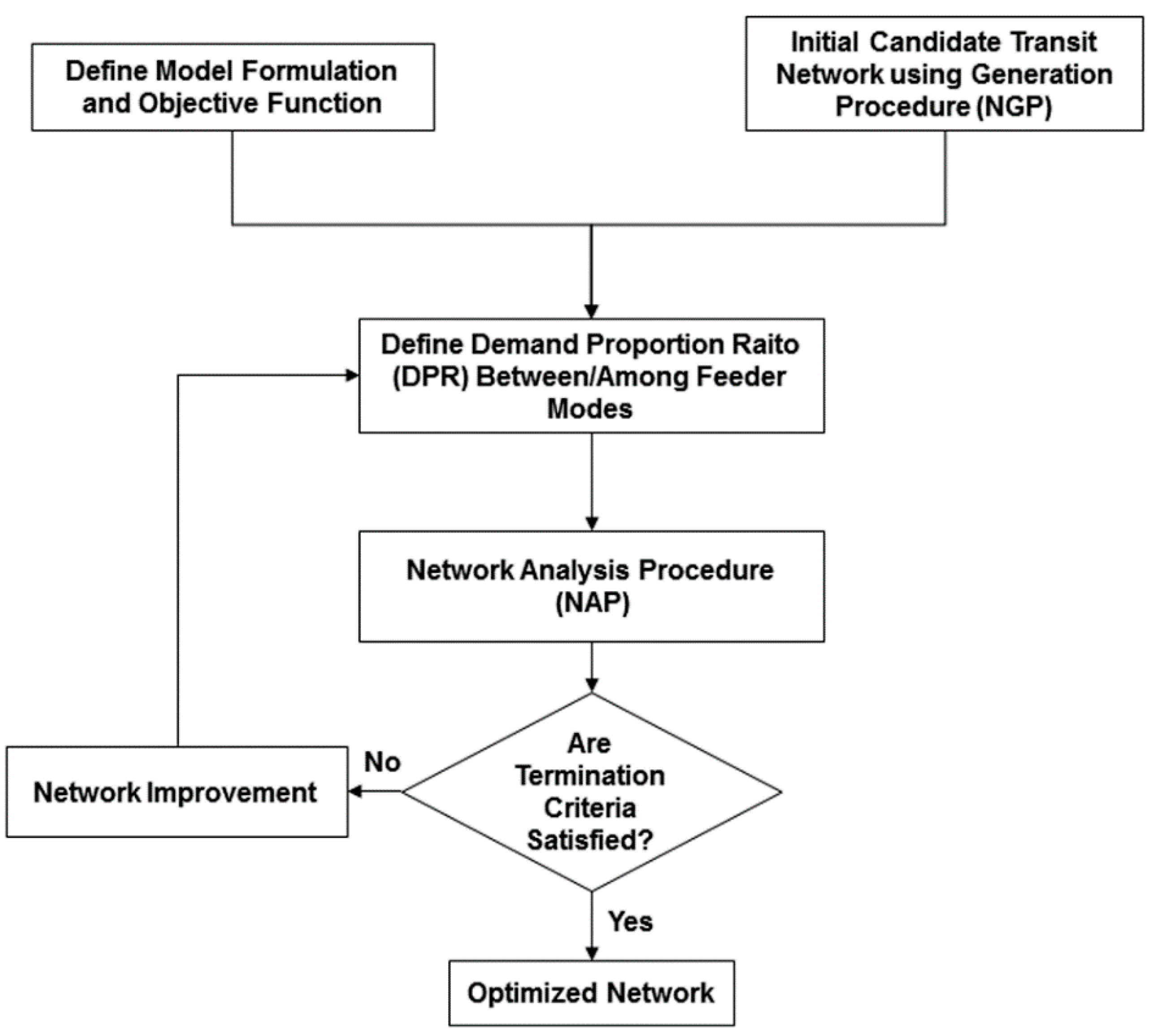
Optimization algorithms: Improvement of the transit network using metaheuristics (e.g., GA and Simulated Annealing (SA)) with respect to the single and multi-objective optimization approaches.

The flowchart of solution framework is demonstrated in Figure 2.

The aforementioned steps are iterated using the optimization algorithms until the termination criterion is met.

3.1. Defining the Objective Function

The total network cost is considered to be the objective function in this study. The total cost of the intermodal transit model is formulated as follows:

C_T = C_u + C_o

(1)

where C_T, C_u, and C_o represent total cost, user cost, and operator cost, respectively. To present the mode more comprehensively, this research considers more cost terms when formulating user costs and operating costs. User cost is related to travelers and is formulated as the product of passengers’ travel times and user’s value of travel time (i.e., value of time for passenger’s waiting and in-vehicle cost).

The operation cost of feeders or railway system was classified into four parts: in-vehicle cost, maintenance cost, fixed and personnel costs. Personnel cost which includes the drivers and administrative costs is dependent on the fleet size, hourly pay, and insurance rate. These cost data come from Mohaymany and Gholami [13]. The cost is formulated as the product of the number of feeders and trains per round trip per each unit of time. In support of nomenclature clarity and convenience purposes, all of the parameters and variables of the formulated intermodal transit model are described in

Table 1. Description of used parameters in the proposed model.

Parameters	Description	Unit
CT	Total system cost	($/h)
Cu	User cost	($/h)
Co.	Operation cost	($/h)
Ca	Accessing cost	($/h)
Cw	Waiting cost	($/h)
Cui	User in-vehicle cost	($/h)
Cf	Fixed costs	($/h)
Coi	Operating in-vehicle cost	($/h)
$C_{duiF}^m$	Dwell user cost of feeder mode m	($/h)
$C_{duiT}^m$	Train dwell user cost	($/h)
Cm	Maintenance cost	($/h)
Cp	Personnel cost	($/h)
AF	Average frequency of feeder	(veh-h)
${\mu }_a^m$	Unit passenger accessing cost of feeder mode m	($/passenger-h)
${\mu }_w^m$	Unit passenger waiting cost for arrival of feeder mode m	($/passenger-h)
${\mu }_I^m$	Unit passenger riding cost on feeder mode m	($/passenger-h)
${\lambda }_f^m$	Unit fixed cost of mode m	($/veh-h)
${\lambda }_l^m$	Unit vehicle operating cost of feeder mode m	($/veh-km)
${\lambda }_I^m$	Unit vehicle operating cost of feeder mode m	($/veh-h)
${\lambda }_{mf}^m$	Unit maintenance cost of feeder mode m	($/veh-km)
${\lambda }_p^m$	Unit personnel cost of feeder mode m	($/veh-h)
${\lambda }_{lT}^m$	Unit operating cost of train	($/veh-h)
$V_{}^m$	Average operating speed of feeder mode m	(km/h)
$S_{kj}^m$	Slack time of route kth at station jth for feeder	(h)
$t_{aF}^{}$	Average accessing time to get to the stop of feeder mode m	(h)
$t_{aTj}^{}$	Average accessing time to reach to the rail station jth via feeder mode m	(h)
$t_{dT}^{}$	Dwell time for boarding and alighting from the train	(h/passenger)
$T_{Tj}$	Linked riding time among station jth and train destination	(h)
$t_{dF}^m$	Dwell time for boarding and alighting from the feeder mode m	(h/passenger)
$t_{ih}^m$	Linked in-vehicle time between nodes ith and hth of feeder mode m	(h)
$T_k^m$	Linked in-vehicle time of route kth for the feeder mode m	(h)
$F_{opt,k}^m$	Optimum frequency of feeder mode m on route kth	(veh/h)
$F_{req,k}^m$	Required frequency of feeder mode m on route kth	(veh/h)
$F_k^m$	Frequency of feeder mode m on route kth	(veh/h)
$F_T^{}$	Optimum frequency of trains	(veh/h)
$f_{\min }^m$	The minimum frequency of feeder mode m	(veh/h)
$f_{\max }^m$	The maximum frequency of feeder mode m	(veh/h)
$N_{}^m$	Total fleet size of feeder mode m	(veh)
LF	Load factor of feeder mode m	(passenger/seat)
$C_{}^m$	Capacity of feeder mode m	(passenger/veh)
$l_{\min }^m$	The minimum length of one route for feeder mode m	(km)
$l_{\max }^m$	The maximum length of one route for feeder mode m	(km)
$V_T^{}$	Average operating speed of train	(km/h)
$T_T^{}$	Train link travel time from 51 to 54	(h)
$q_{nk}^m$	Demand of node nth in route kth of feeder mode m	(passenger/h)
$N_k^m$	Number of stops in route kth of feeder mode m	-
Q	Total demand	(passenger/h)
$q_i^m$	Demand of feeder mode m at node ith	(passenger/h)
$Q_k^m$	Demand of route kth of feeder mode m	(passenger/h)
$l_{ih}^{}$	Travel distance from node ith to hth	(km)
$L_{ijk}^m$	Travel distance from each stop ith to station jth in route kth of feeder mode m	(km)
$L_k^m$	Length of route kth for the feeder mode m	(km)
$X_{ihk}^m$	Binary variable; value of 1 if stop ith precedes stop hth on route kth of mode m	-
$Y_{ij}^m$	Binary variable; value of 1 if stop ith is assigned to station jth via mode m	-
I	Number of stops	-
J	Number of stations	-
M	Number of feeder mode
NR	The maximum number of routes in feeder modes	-
H	Any proper subset of I + J, containing all stations	-

.

The total network cost of the intermodal transit model includesoperation parameters, user parameters, and decision variables. The objective function is specified as the sum of the operating and user costs, which is presented in the following equation:

$$Minimize\begin{array}{c}\end{array}{C}_T=\left[\stackrel{User}{\overbrace{\left(C_a^{}+C_w^{}+C_{ui}^{}\right)}}+\stackrel{Operating}{\overbrace{\left(C_f^{}+C_{oi}^{}+C_m^{}+C_p^{}\right)}}\right]$$

(2)

Consequently, the mathematical formulation of all cost terms substitution can be presented as given:

$$Minimize\hspace{1em}{C}_T={\displaystyle \sum _{m=1}^M\left[\begin{array}{l}{\mu }_{{}_a}^m\left(t_{aF}{\displaystyle \sum _{i=1}^I{q}_{{}_i}^m}+{\displaystyle \sum _{j=1}^J{t}_{aTj}{\displaystyle \sum _{i=1}^I{q}_{{}_i}^m\times Y_{{}_{ij}}^m}}\right)+{\mu }_{{}_w}^m\left({\displaystyle \sum _{k=1}^{K^m}\left[\left(\frac{1}{2F_k^m}+\frac{1}{2F_T}\right)\times Q_{{}_k}^m\right]}\right)+{\lambda }_{IT}^{}\left({\displaystyle \sum _{i=1}^I{q}_{{}_i}^m\times t_{dT}}+\left(2F_T\times T_T\right)\right)+\\ {\mu }_{{}_I}^m\left({\displaystyle \sum _{k=1}^{K^m}\left[{\displaystyle \sum _{i=1}^I{q}_{{}_i}^m{\displaystyle \sum _{j=1}^J{T}_{{}_{ijk}}^m}}+{\displaystyle \sum _{n=1}^{N^k}{q}_n^m\left({\displaystyle \sum _{n=n+1}^{N^k}{q}_n^m+1}\right)\times t_{dF}^m}\right]}+{\displaystyle \sum _{j=1}^J{\displaystyle \sum _{i=1}^I{q}_{{}_i}^m\times Y_{{}_{ij}}^m}\left[T_{Tj}+\left({\displaystyle \sum _{j=j+1}^J{\displaystyle \sum _{i=1}^I{q}_{{}_i}^m\times Y_{{}_{ij}}^m}+1}\right)\times t_{dT}\right]}\right)+\\ \left({\lambda }_f^m+{\lambda }_p^m\right){\displaystyle \sum _{k=1}^{K^m}\left[\left(2F_k^m\times T_k^m\right)+\left(Q_k^m\times t_{dF}^m\right)+\left(F_k^m\times S_{kj}^m\right)\right]}+{\lambda }_I^m{\displaystyle \sum _{k=1}^{K^m}{Q}_k^m\times t_{dF}^m}+\left({\lambda }_l^m+{\lambda }_{mF}^m\right){\displaystyle \sum _{k=1}^{K^m}2F_k^m}\times L_k^m\end{array}\right]}$$

(3)

which is subject to

$${\displaystyle \sum _{k=1}^{K^m}{\displaystyle \sum _{h=1}^{I+J}{X}_{{}_{ihk}}^m}}\le 1\begin{array}{cc}& \end{array}i=1,\dots ,I\begin{array}{cc}& \end{array}m=1,\dots ,M$$

(4)

$${\displaystyle \sum _{i=1}^I{\displaystyle \sum _{j=I+1}^{I+J}{X}_{{}_{ijk}}^m}}\le 1\begin{array}{cc}& \end{array}k=1,\dots ,K^m\begin{array}{cc}& \end{array}m=1,\dots ,M$$

(5)

$${\displaystyle \sum _{h=1}^{I+J}{X}_{ihk}^m-{\displaystyle \sum _{d=1}^I{X}_{dik}^m}}\ge 0\begin{array}{cc}& \end{array}i=1,\dots ,I\begin{array}{cc}& \end{array}k=1,\dots ,K^m\begin{array}{cc}& \end{array}m=1,\dots ,M$$

(6)

$${\displaystyle \sum _{i\notin H^{}}{\displaystyle \sum _{h\in H^{}}{\displaystyle \sum _{k=1}^{K^m}{X}_{{}_{ihk}}^m}}}\ge 1\begin{array}{cc}& \end{array}m=1,\dots ,M\begin{array}{cc}& \end{array}\forall H^{}$$

(7)

$${\displaystyle \sum _{h=1}^{I+J}{X}_{{}_{ihk}}^m+}{\displaystyle \sum _{d=1}^I{X}_{dik}^m}-Y_{{}_{ij}}^m\le 1\underset{\begin{array}{cc}& \end{array}}{\overset{}{{\displaystyle }}}i=1,\dots ,I\underset{\begin{array}{cc}& \end{array}}{{\displaystyle }}j=I+1,\dots ,H\underset{\begin{array}{cc}& \end{array}}{\overset{}{{\displaystyle }}}k=1,\dots ,K^m\underset{\begin{array}{cc}& \end{array}}{\overset{}{{\displaystyle }}}m=1,\dots ,M$$

(8)

$$l_{\min }^m\le L_{{}_{{}_K}}^m\le l_{\max }^m\begin{array}{cc}& \end{array}m=1,\dots ,M\begin{array}{cc}& \end{array}k=1,\dots ,K^m$$

(9)

$$f_{\min }^m\le F_k^m\le f_{\max }^m\begin{array}{cc}& \end{array}m=1,\dots ,M\begin{array}{cc}& \end{array}k=1,\dots ,K^m$$

(10)

$${\displaystyle \sum _{k=1}^{K^m}\left[\left(2F_k^m\times T_k^m\right)+\left(Q_k^m\times t_{dF}^m\right)+\left(F_k^m\times S_{kj}^m\right)\right]}\le N^m\begin{array}{cc}& \end{array}m=1,\dots ,M$$

(11)

$${\displaystyle \sum _{r=1}^{R^m}{r}_{}^m}\le NR\begin{array}{cc}& \end{array}m=1,\dots ,M$$

(12)

Decision variables include two binary variables, $X_{ihk}^m$ and $Y_{ij}^m$, whichrepresent the transit network configuration, as shown in Table 1. Other decision variables are demand ratio for each feeder stop amongst the feeder modes at stops ($q_i^m$), and feeder frequency of each route in each mode ($F_k^m$).

The first term in Equation (3) is the access cost for multimode transit passengers, which is the production of local demand, with the value of time and accessing time.

The second term that is seen in Equation (3) is user waiting costs, which contains passengers that are waiting for the feeders and trains.

The third term in Equation (3) relates to the operating cost for a rail service, which depends on passenger demand, fleet size of the rail network, and route station distance. The derivation of this cost is indictedin the literature in detail [10].

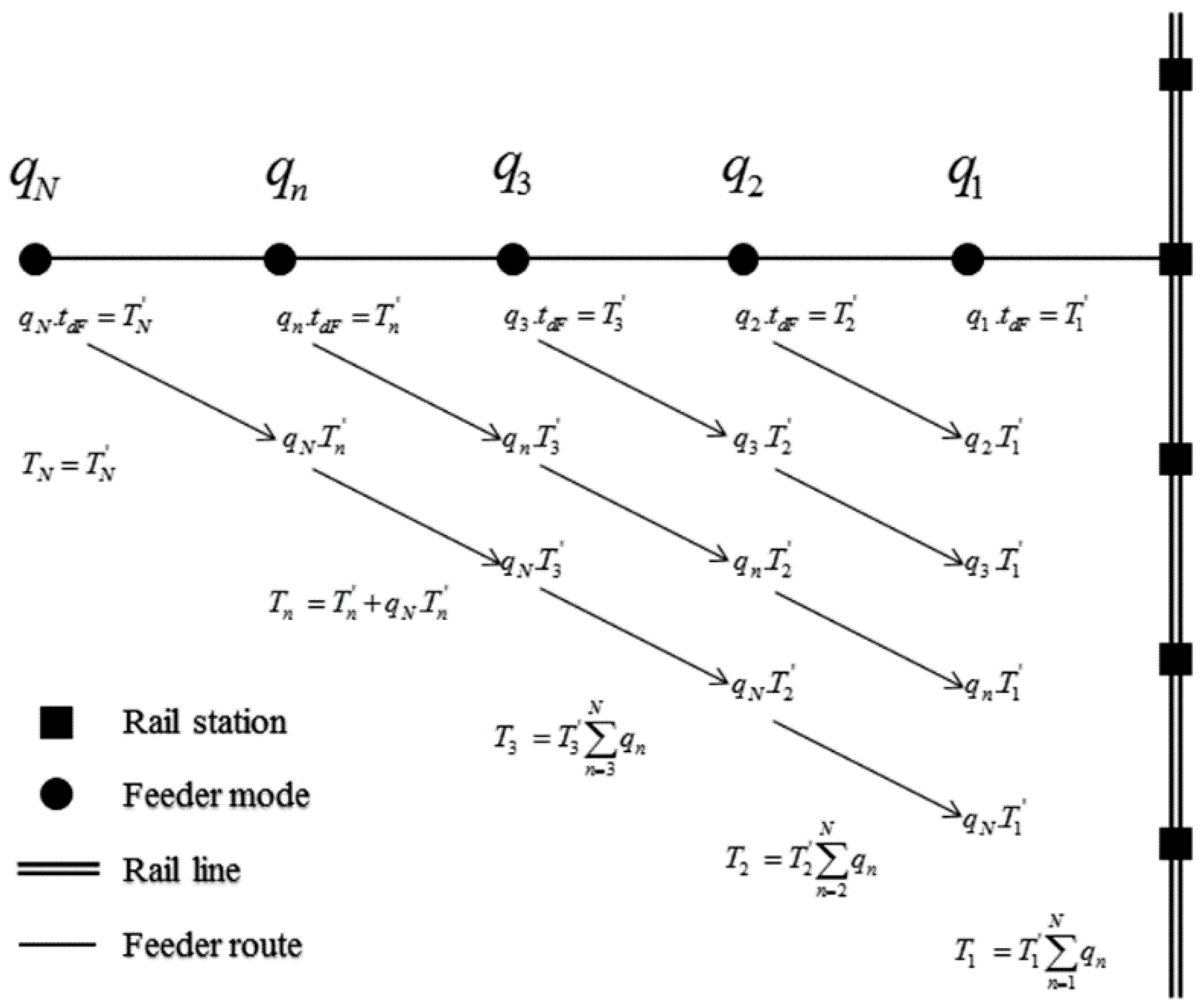
The fourth and fifth terms given in Equation (3) are user in-vehicle costs, which contain in-vehicle time, passenger demand, and the value of user in-vehicle time. This cost, C_ui, is formulated based on the average trip time and is determined in two main parts: the user dwell time and the user running time.

Dwell time is the time that a vehicle stays at the bus stop to load/unload other passengers. When considering the variation in time spent, the geometric series equation presentedby Almasi et al. [10,11] has been revised in this study. Figure 3 demonstrates the actual condition for traveler demand and dwell time at each feeder stop along the route, rth, connected to the rail station.

As shown in Figure 3, the dwell time distribution depends on demand at each stop along the route. q_n denotes the demand at feeder stop, nth, in the feeder route. T_n is user dwell time because of demand, q_n. At feeder stop n − 1, the boarding and alighting time (T_n−1) will be imposed to the passenger demand of nth feeder stop (q_n). Consequently, the dwell time will be increased by increasing passenger demand in consequent feeder stops. Therefore, the dwell user cost of route, kth, and feeder mode, mth, is formulated with the summation of dwell time for demand at each feeder stop and unit time value, as follows:

$$C_{duiF}^m={\mu }_{{}_I}^m\left[q_1^m\times \left(1+q_2^m+\dots +q_N^m\right)+q_2^m\times \left(1+q_3^m+\dots +q_N^m\right)+\dots +q_N^m\right]$$

(13)

Therefore, formulation of the network dwell cost is obtained as follows:

$$C_{duiF}^m={\mu }_{{}_I}^m\left({\displaystyle \sum _{n=1}^{N_k^m}{q}_{nk}^m\left[{\displaystyle \sum _{n=n+1}^{N_k^m}{q}_{nk}^m+1}\right]\times t_{dF}^m}\right)$$

(14)

Similarly, spending dwell time at each rail station is different. Therefore, the number of traveler and dwell cost would be different. Figure 4 demonstrates the real situation of trip demand at each rail station.

$Q_j^{}$ denotes the passenger demand at rail station, jth, in the rail line. T_j is user dwell time by demand, $Q_j^{}$. The boarding and alighting time at station j − 1 (T_j−1) will be imposed to the demand of jth station ($Q_j^{}$). Consequently, the dwell time will be increased by increasing the demand in consequent rail stations. $C_{duiT}^m$ for every feeder vehicle is calculated by summation of dwell time for demand at each station and unit time value. Therefore, the train user dwell cost is determined as follows:

$$C_{duiT}^m={\mu }_{{}_I}^m\left[Q_1^m\times \left(1+Q_2^m+\dots +Q_J^m\right)+Q_2^m\times \left(1+Q_3^m+\dots +Q_J^m\right)+\dots +Q_J^m\right]\times t_{dT}$$

(15)

Thus, network user dwell cost for trains can be formulated as follows:

$$C_{duiT}^m={\mu }_{{}_I}^m\left({\displaystyle \sum _{j=1}^J{\displaystyle \sum _{i=1}^I{q}_{{}_i}^m\times Y_{ij}}\left[{\displaystyle \sum _{j=j+1}^J{\displaystyle \sum _{i=1}^I{q}_{{}_i}^m\times Y_{ij}}+1}\right]\times t_{dT}}\right)$$

(16)

Therefore, the dwell user cost for feeders and trains, for each mode, m, is given as:

$$C_{dui}^m={\mu }_{{}_I}^m\left({\displaystyle \sum _{k=1}^{K^m}{\displaystyle \sum _{n=1}^{N_k^m}{q}_{nk}^m\left[{\displaystyle \sum _{n=n+1}^{N_k^m}{q}_{nk}^m+1}\right]\times t_{dF}^m+{\displaystyle \sum _{j=1}^J{\displaystyle \sum _{i=1}^I{q}_{{}_i}^m\times Y_{ij}}\left[{\displaystyle \sum _{j=j+1}^J{\displaystyle \sum _{i=1}^I{q}_{{}_i}^m\times Y_{ij}}+1}\right]\times t_{dT}}}}\right)$$

(17)

The operating costs, formulated as the sum of C_oi, C_m, C_p, and C_f, are presented in the sixth to eighth terms of Equation (3). To improve accuracy, the dwell time and feeder-mode slack time are used in this study. The stop delay time incurred at feeder stops, and the running cost for the feeders is defined according to the round trip link time.

The route feasibility in the network design in terms of the constraints for the MFNDP would confirm by Equations (4)–(8). These constraints are used by previousstudies [9,14,15]. Equation (9) represents constraints on the minimum and maximum length of feeder routes. Similarly, limitations for the minimum and maximum frequencies are specified in Equation (10), while Equation (11) shows the maximum allowable number of vehicles in the fleet. Equation (12) presents the restriction for the maximum number of routes in the proposed multimode network.

Equations (9)–(12) represents the constraints on the length of feeder routes, limitations for the frequencies, allowable number of vehicles in the fleet, and the maximum number of routes in the proposed multimode network.

3.2. Network Generation Procedure

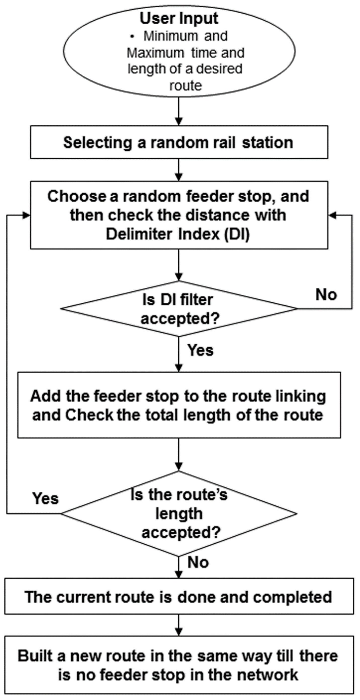
To identify a candidate network, a network generation module is designed. All of the routes are built as described below.

First, a rail station is chosen at random, subsequently, stops, selected at random, are added to the path linking to this rail station. The length of the path is checked after adding each stop. The current path is terminated if it exceeds the maximum length (L_max) and a new path will be constructed in the same way. The process continues until all the stops have been contained in the network.

Random selection of stops with no restrictions may create a poor initial solution. Thus, the concept of delimiter proposed by Breedam [16] is developed in this study. The delimiter is applied to both station to the first bus stop, and bus stop to the next bus stop as given below.

(a)

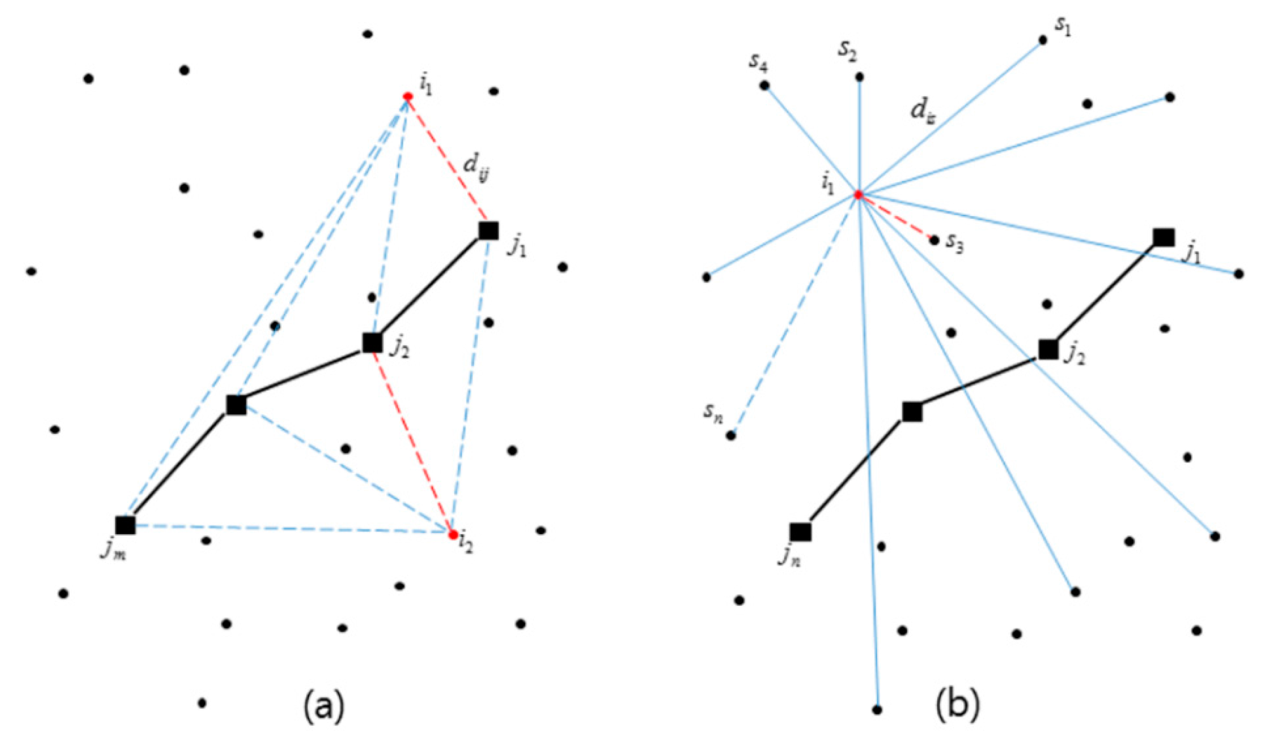
Station to the first bus stop: A selection constraint in terms of the distance among the stations and stops is a delimiter. The delimiter is determined as shown in Equations (18) and (19) below.

For each feeder stop, ith, define the distance of its nearest rail station, jth ($Dis{t}_{{}_i}^F$), using:

$$Dis{t}_i^F=\underset{j}{\min \begin{array}{c}\end{array}}{d}_{ij}$$

(18)

The initial delimiter DI^F is equivalent to the maximum of the set of minimum distances determined as given by (see Figure 5a):

$$DI=\underset{i}{\max \begin{array}{c}\end{array}}(Dis{t}_i^F)$$

(19)

Therefore, the distance among the selected rail station and bus stops should be less than or equal to DI^F, otherwise a new stop will be selected. Similarly, the delimiter will intercept to link a station and a stop that are too far apart.

(b)

One bus stop to the next bus stop: Similarly, a range delimiter in order to narrow the search distance among the selected random stops and the stops is provided. This range delimiter prevents the selection of a sequence of stops that exceed the allowable distance (see Figure 5b):

$$Dis{t}_i^b=\underset{s\in I}{\min \begin{array}{c}\end{array}}{d}_{is},\begin{array}{cc}& \end{array}i\notin s$$

(20)

$$D{I}^B=\underset{i}{\max \begin{array}{c}\end{array}}(Dis{t}_i^B)$$

(21)

The stop sequence in each route is reordered to reduce the route distance, which in turn, may reduce the total cost. In addition, a flowchart of the initial candidate network using the NGP is presented in Figure 6.

3.3. Defining Demand Proportion Ratio among/between Modes

Another purpose of the proposed MFNDP is to determine the optimal demand proportion for feeder modes at each stop when considering the minimum total cost in the transit system. Normally, after network optimization, the feeder mode will be decided at each route.

The objective function shows the impact of the demand density at each stop and network configuration on dwell user cost. At each network configuration, the amount of passenger demand at each bus stop highly influences the total cost. Therefore, importance ofthe demand ratio among the feeder modes at each bus stop based on the network configuration is understood.

In the proposed strategy, an optimum demand proportion among the modes at each bus stop has been found. This strategy helps to create a more flexible transit network with any range of demand density. To identify the demand ratio amongst the feeder modes at each bus stop (q_i^m) as decision variables, an inner optimization task has been performed using a metaheuristic approach on the given network.

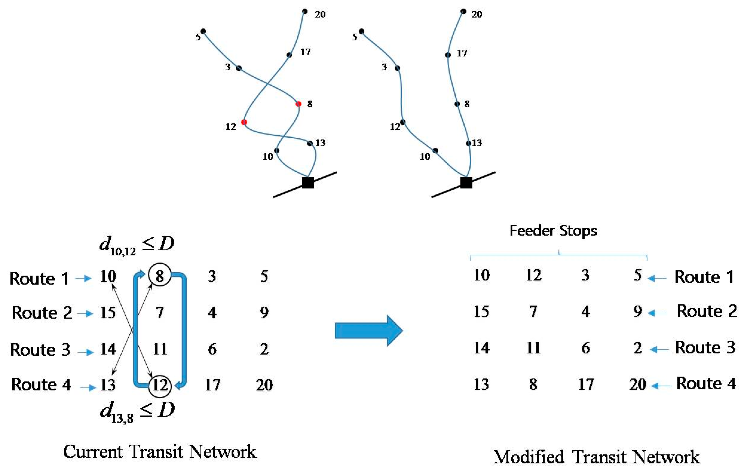
The network information, total demand at each bus stop, and the design parameters are given as input data. However, DPR at each bus stop are defined as decisions. Figure 7 shows an example of the demand proportion ratio and modified routes on a simple network. The input network presents two routes for mode one ($R_{{}_1}^{m1}$ and $R_2^{m1}$) and two routes for mode two ($R_{{}_1}^{m2}$ and $R_2^{m2}$). Metaheuristic approaches determine the optimal demand ratio of the demand at each bus stop. Based on the defined DPR at each bus stop, the network will be modified and cost will be evaluated based on the new proposed transit network (see Figure 7).

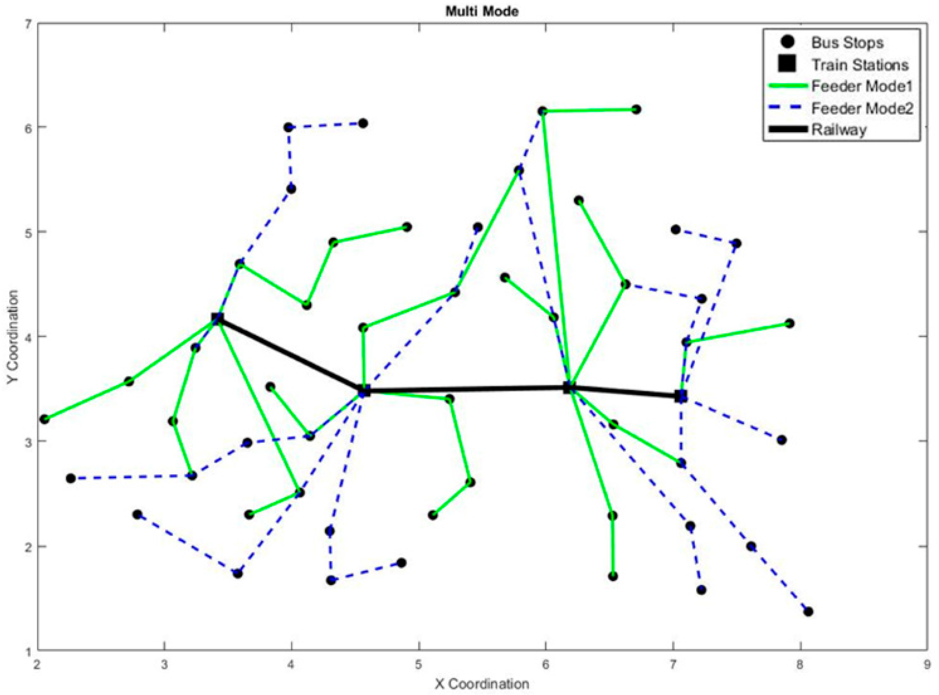
The proposed approach includes M feeder modes (e.g., bus and van) with different characteristics connected to coordinated mass transit services that will provide a more sustainable flexible network. Figure 8 illustrates an example of MFNDP after the DPR and modification on the given network. Some stops are served by only one feeder mode, while others are served by both feeder modes that are based on the designated DPR.

3.4. Network Analysis Procedure

A process to analyze, evaluate different network structures, and conclude their associated route service frequencies is described by NAP. Input data for the NAP contains the following items:

(a)

Transit network information includes the location and the number of the nodes where the trip demand originates and/or heads on the routes that are connected with each node through connectors. The proposed solution network can be generated using a heuristic process (NGP) or using metaheuristic optimizers.

(b)

Demand data, which includes a demand matrix expressing the number of travelers that are using transit and DPR between/among feeder modes at each bus stop.

(c)

Design parameters that refer to some parameters that are identified by the plannerssuch as load factor at each route, the feeder capacity, the maximum number of bus routes, cost parameters, and so forth.

Once a specific transit network is proposed by NGP or network improvement, NAP is utilized to evaluate the different network and calculate route frequencies. NAP procedure can be illustrated as follows.

First, a trip assignment is employed to assign the trip demand to specified routes associated through the presented multimodal transit network configuration. Then, F_k for each route is calculated using the frequency setting procedure. The optimum F_k isrelated to the transit network configuration. The analytical approach is used to determine the optimum F_k by setting the first derivative of the cost function with respect to the feeder mode frequency, equating it to zero, and solving it. Thus, the optimal feeder frequency can be formulated as follows:

$$F_{{}_{opt,k}}^m=\sqrt{\frac{{\mu }_{{}_w.}^m{Q}_k^m}{4L_k^m\left[\left({\lambda }_l^m+{\lambda }_{mF}^m\right)+\frac{1}{V_k^m}\left({\lambda }_f^m+{\lambda }_p^m\right)\right]+2S_{kj}^m\left({\lambda }_f^m+{\lambda }_p^m\right)}}$$

(22)

Moreover, the minimum required frequency for route, kth, is taken as follows:

$$F_{{}_{req,k}}^m=\frac{Q_k^m}{L{F}^m\times C^m}$$

(23)

The given frequency for route, kth, is acquired by choosing the maximum value of F_req,K and F_opt,K as shown in Equation (24):

$$F_k^m=\max (F_{{}_{req,k}}^m,F_{{}_{opt,k}}^m)$$

(24)

Then, the output data show the optimal transit network design, service frequencies, and demand information, with an extensive variety of performance measures. Figure 9 gives the flowchart for NAP.

3.5. Improvement Strategy

In this research, we have applied several operators in order to modify/change/amend a multimodal transit network, as given in the following sections. Also, a criterion for choosing the neighborhood has been suggested.

3.5.1. Delimiter Value

Usually, the stops required to perform the move are selected at random. In this case, because of the large search space, a number of bad move selections can be involved.

In order to narrow the search space and make the process more intelligent, a criterion, called the range delimiter, has been proposed to prevent the selection of too many bad moves (Breedam 2001). The concept of delimiter value is similar to the generation of an initial solution described in the previous Section.

The range of delimiter is equal to the travel distance limitation between nodes of the different routes selected at random for the move. This travel distance limitation is calculated for each solution network with k routes (R₁, R₂, …, R_k), as given in Equation (25) below.

First, wecalculated the distance (i.e., Euclidian distance) between stop, ith, in route, R_k, and its nearest neighboring stop, jth, belonging to another route, R_m:

$$N{N}_i=\underset{j\notin R_k}{min} d_{ij}\begin{array}{cccc},& & & i\in R_k\end{array}$$

(25)

$$D=\underset{i}{\max } N{N}_i$$

(26)

Therefore, the distance between the stops of two different routes selected at random for the exchange move must be less than the delimiter value (D), so that in this case there is a higher potential for generating a move that will improve the quality of the neighborhood solution. Hence, to prevent bad moves by choosing far distance stops, the delimiter value strategy has been carried out for every proposed operator.

3.5.2. Defining Neighborhood Moves

Number of solutions defines by the neighborhood structure that can be achieved in one single or multiple move(s) from a current solution. These types of moves are aimed at improving a feasible solution by moving feeder stops within or between/among routes. The purpose is to rearrange the feeder stop sequence in every single route and transit network to reduce the total cost.

Five types of moves are considered in this paper. They are the swap operator, insertion operator, single-point crossover operator, uniform crossover operator, and mixed operator. Figure 10 shows an example of each of first four operators. Mixed operator is a combination of those four operators. All of the operators are applied only for feeder stops and we assumed that for a candidate transit network rail stations are fixed. The details of operators used are represented below.

Swap operator:The swap operator exchanges the positions of two feeder stops from two different routes in a particular column. However, in this paper, the swap operator used is equal to the maximum number of stops in a route in a given MFNDP. In fact, for each column of a transit network, one single swap operator is utilized.

It is worth mentioning that the choice of stops for a swap operator is performed using the strategy given in the section of delimiter value for both previous and selected feeder stops. If the distance between a selected stop and the previous feeder stop is equal to or smaller than the D, then the swap operator can be appliedfor that particular column. Hence, the feeder stops are chosen at random, while their new positions depend on the delimiter criterion. This concept is applied to all of the operators that are considered in this paper. Figure 11 demonstrates an accepted move using the swap operator.

Insertion operator: The insertion operator tries to improve the transit network by removing a stop from a route and inserting it into another route in a particular column. There is difference between the swap and insertion operators. In the insertion operator, a stop is removed from a route and is added to another route, while in the swap operator, stops are exchanged. Similar to the swap operator, the insertion operator obeys the concept of delimiter value for both stops and rail stations (see Figure 12). If the delimiter condition is satisfied, then the insertion operator is allowed to be applied.

Swap operator is applied equal to the maximum number of stops in a route in a given MFNDP. As MFNDP aims to minimize the total cost, while satisfying network constraints, a candidate transit network with a large number of routes may not provide an appropriate transit network. Figure 10b depicts the application and usefulness of this operator in practice.

Single-point crossover operator: By selecting two random routes, a single cut (point) is randomly chosen. After selecting two routes and a single cut number, if the delimiter value (D) condition allows, two strings of stops can be exchanged at a given cut number. The delimiter criterion should be checked for both stops, locating as first stop in strings to be allowed for exchange purpose. Figure 13 depicts a successful exchange using the single-point crossover over two different routes. Furthermore, a schematic view of this operator is shown in Figure 10c.

Uniform crossover operator: For the uniform crossover operator, as for the single-point crossover, two random routes from the transit network are selected. Then, between two selected routes, the route with a minimum number of stops is taken as the reference route, and the other one is called the subject route. Based on the basic concept of uniform crossover, a random binary vector is generated as a decision vector in which 1 means ‘exchange’ and 0 means ‘do not exchange’.

Based on the binary decision vector, the reference and subject routes collaborate with each other. An example of this operator is given in practice, as shown in Figure 10d. Figure 14 illustrates the process of this useful operator.

Mixed Operator: The mixed operator is a combination of the swap, insertion, single-point, and uniform operators in one single update for the transit network. In fact, using the mixed operator, all the good chances gather in one place; however, using this operator too many times may increase the chance of getting stuck in local optima. In applying the aforementioned operators, we have used unbiased selection and equal chance for each operator. Next, brief and concise explanations of the applied optimizers are provided.

4. Applied Optimization Algorithms

Metaheuristic optimization algorithms have shown their capabilities for finding the near-optimal solution to the numerical real-valued test problems for which exact and analytical methods may not be able to produce within a reasonable computation time, especially when the global minimum is surrounded by many local minima. Network design problem has been known to be NP-complete, so it would be proper to apply metaheuristic approach in real-world size network problems.In this section, the metaheuristic optimization algorithms that are used to modify/improve the multimodal transit network have been explained in brief.

4.1. Genetic Algorithms

GA is categorized as evolutionary optimization algorithms and is considered as one of the widely used optimizers in the literature. The basic idea of GA first proposed by Holland [17]. The GA is based on the process of evolution by natural selection seen in nature. Indeed, evolution shows selection and replication of better solutions. Simplicity of concept and usage may be considered as an advantage in theefficiency of GA for solving complicated optimization problems [18].

Regarding the search operators used in GA, crossover, mutation, and selection strategy are the most important factors. Like other population based optimization method, GA starts with an initial population of individuals, the so called population of chromosomes. Usually, initial population randomly generated at starting of the optimization task in the most optimizers as for GA. Population size is a user parameter value and can be varied from few chromosomes to thousands ones.

Next, is function evaluation process to see how fit/good the solutions are based on the cost/fitness function defined by given problem. After calculating the fitness/cost function, the selection strategy should be defined due to selection process of parents for creating offspring using the crossover search operator. Selection process tries to choose the best solutions among (between) other solutions. There are different methods for selection process, such as roulette wheel selection, however the fundamental idea is the same, selecting better individuals with a higher chance to be selected for the next generations.

In this step, after selecting better chromosomes, crossover operator will be applied by combining some aspects of selected individual. For instance, from two selected parents, two offspring will be generated by transferring their features, then, a population of offspring can be formed. However, for having more diversity in the population of chromosomes, mutation search operator is applied with little bit randomness into the population features. The ratio of mutation rate is a small number and will apply to the entire population with a random selection. Finally, by combining three populations, including the current population, populations that are formed using crossover and mutation, we have a new population having more than the predefined population size. After sorting the new combined population, only chromosomes that are equal to the size of population will be kept and the rest of chromosomes will be discarded from the optimization task. The aforementioned processes will continue till the stopping condition is met.

4.2. Simulated Annealing

SA is inspired by the annealing process, the process of slow cooling of a hot metal. This inspiration first proposed in 1953 introducing a new optimization technique for solving global optimization problems [19].

The concept and implementation of SA is easy to understand and apply, and that is why this optimization method is one of the well-known optimization methods for solving both continuous and discrete problems. Back to the annealing process, by increasing the temperature in a metal, its atoms start to move around with large movements. By slow cooling of the metal, the atoms have sufficient time to allocate in their best location in finding the lowest level of energy, resulting in better metal in terms of strength and durability.

The SA simulates the aforementioned slow cooling process by a small random movement of an atom. Regarding the application point of view, energy level is resembled as objective function. The optimization task starts at high temperature. If the new change resulting in negative energy state, then the applied movement is accepted. However, if the new change applied by the small displacement is resulted in positive energy state, then, with a probability, there would be a high chance to accept the applied small displacement. The Boltzmann probability is used for this selection, given as follows [20]:

$$P=\exp \left(\frac{-\Delta E}{kT}\right)$$

(27)

where k and T are the Boltzmann constant and the current temperature, respectively. The variable ΔE plays the role of cost function (fitness function) used in SA approach and it means that the difference of objective functions (current cost–previous cost). Equation (27) will be compared with a random uniform distribution value between zero and one. If the random value is smaller than the Boltzmann probability, then the new change is accepted. As the temperature reduces, the chance of selecting bad moves will decrease till at final iterations, almost no bad configurations would be accepted aiming for having more exploitation [21].

Although, the SA would be computational expensive in finding global optimum point, however, it can find near optimum solution with fewer design evaluations when comparing with other existing optimizers.

4.3. Water Cycle Algorithm

The basicinspiration of the water cycle algorithm (WCA) is derived by water cycle process in nature and is based on the observation of how rivers and streams flow into the sea. Indeed, the WCA tries to formulate the surface runoff of streams and rivers seen in nature. The WCA starts with an initial population called the population of streams. First, let us assume that raining has been happened. Afterwards, the best individual which is the best stream is selected to be as a sea in the WCA model [22].

Afterwards, the initial population is sorted and due to choosing rivers and sea, a predefined number of best streams (N_sr) are considered to be as rivers. Based on their intensity of flow, water from the streams is absorbed to the rivers and sea. Also, it would be possible for some streams directly flow into the sea. Therefore, new movement formulations for streams and rivers are suggested, as follows.

$${\overrightarrow{X}}_{Stream}^{i+1}(t+1)={\overrightarrow{X}}_{Stream}^i(t)+rand\times C\times ({\overrightarrow{X}}_{River}^i(t)-{\overrightarrow{X}}_{Stream}^i(t))$$

(28)

$${\overrightarrow{X}}_{Stream}^{i+1}(t+1)={\overrightarrow{X}}_{Stream}^i(t)+rand\times C\times ({\overrightarrow{X}}_{Sea}^i(t)-{\overrightarrow{X}}_{Stream}^i(t))$$

(29)

$${\overrightarrow{X}}_{River}^{i+1}(t+1)={\overrightarrow{X}}_{River}^i(t)+rand\times C\times ({\overrightarrow{X}}_{Sea}^i(t)-{\overrightarrow{X}}_{River}^i(t))$$

(30)

where t and rand are an iteration number and a uniformly distributed random number between 0 and 1. In case of finding better solution using new generated streams, the position of streams and its corresponding river will be switched. In fact, Equations (28)–(30) represent the exploration phase in the WCA.

In order to conduct the exploration phase in the WCA, if the Euclidian distance between the sea and a specific stream/river is less than a predefined value (d_max), then, the evaporation condition is applied and a new stream/river can be generated. Figure 15 displays the schematic view of the movement strategy of WCA, where circles, stars, and the diamond resemble to the streams, rivers, and sea, respectively. a and b are current distance between a stream and new position of an updated stream, and its corresponding river, respectively [23].

4.4. Non-Dominated Sorting Genetic Algorithm II

Non-dominated sorting strategy has been used for converting GA into an efficient multi-objective optimizer. The optimization strategy behind of Non-dominated Sorting Genetic Algorithms II (NSGA-II) is based on the standard GA. The selection process in the NSGA-II is based on the binary tournament selection with replacement as for GA. Regarding the exploration phase; a random mutation operator is applied to a small portion of solution to ensure searching unobserved regions.

If the new generated solution does not satisfy the applied constraints during recombination and/or mutation operators, the solution is ignored and another new solution will be created using the aforementioned operators until a feasible solution is obtained. For evaluating the fitness function, there are two steps. Talking about the first step, as the name of non-dominating approach shows, the solutions are ranked based on Pareto dominance.

After sorting based on the rank scores, the solutions are sorted based on their crowding distance values. In the crowding distance mechanism, the extreme values for each objective are assigned infinite values, for keeping these values as best solutions [24]. The rest of the search operators that are used in NSGA-II, such as crossover and mutation, act the same in GA.

4.5. Non-Dominated Sorting Water Cycle Algorithm

The non-dominated sorting WCA (NSWCA) as for NSGA-II has used the concept of non-dominated sorting strategy as its name represents. In standard WCA, only one objective function should be minimized or maximized and in this situation, a number of best obtained solutions are chosen as the sea and rivers. However, for multi-objective optimization problems (MOPs), there is more than one function to be minimized or maximized.

Therefore, the multi-objective version of WCA needs to be modify enabling selection of the sea and rivers in the multi-objective space. Due to find the best solutions including sea and rivers for each population (iteration), a crowding distance mechanism introduced by Deb et al. [24] is utilized.

Proper selection of sea and rivers (few obtained best solutions) affects both the convergence capability of the NSWCA, as well as the ability to maintain a good distribution of non-dominated solutions [25]. Therefore, for all of the iterations, solution having the highest crowding-distance values should be determined nominating as sea and rivers in order. Also, the magnitude of flow for the rivers and sea are evaluated using the concept of crowding-distance mechanism [25].

Moreover, the non-dominated solutions have been saved in an archive to generate the Pareto front sets. This archive is updated at each iteration, and dominated solutions are removed from the archive by iteration continues. As it obvious, new found non-dominated solutions will be added to the Pareto archive.

However, there is a limitation of the size of Pareto archive, which is a user parameter in the MOPs. Therefore, when the number of members in the Pareto archive exceeds the Pareto archive size, the crowding distance strategy will be applied again in order to delete as many non-dominated solutions as necessary.

5. Numerical Results and Discussions

The proposed solution methodology for the MFNDP was applied to the data set in the literature [11]. The case study region is an area of 5.5 × 6.5 km² in the south of Petaling Jaya in Malaysia, and included the Kelana Jaya Line at Kuala Lumpur railway. There were four stations in the study area.

A total of 54 nodes is defined to describe the service area and associated network connectivity. All 54 nodes are selected from the existing transit network, which consists of public bus routes with fixed schedules operated by the public transportation companies such as Rapid KL and Metrobus, etc. Network connectivity is generated from street links that connect these 54 nodes and are suitable for bus operations. The generation of the demand matrix is based on a questionnaire survey data collection. By extracting the abstained results from survey, the demand matrix was determined. The parameters are based on the data collection from field as well as ridership and financial reports, which were publicized by Barton [26] and Valley Metro [27].

More information about design-related parameters used in the models is represented in

Table 2. Values of the parameters used in reported study region.

	Unit	Value for Mode 1 (Bus)	Value for Mode 2 (Van)	Value for Train
${\mu }_a^m$	$/passenger-h	8	8	8
${\mu }_w^m$	$/passenger-h	8	8	8
${\mu }_I^m$	$/passenger-h	4	4	4
${\lambda }_f^m$	$/veh-h	14.37	4	-
${\lambda }_l^m$	$/veh-km	0.36	0.07	-
${\lambda }_I^m$	$/veh-h	8.94	1.63	-
${\lambda }_{mf}^m$	$/veh-km	0.75	0.25	-
${\lambda }_p^m$	$/veh-h	10.2	10.2	-
${\lambda }_{lT}^m$	$/veh-h	-	-	180
$V_{}^m$	km/h	25	25	-
$V_{}^T$	km/h	-	-	40
$S_{kj}^m$	min	15	15	-
$t_{aF}^{}$	min	7.5	7.5	-
$t_{aTj}^{}$	min	-	-	4
$t_{dT}^{}$	min/passenger	-	-	0.03
$t_{dF}^m$	min/passenger	0.096	0.15	-
$F_T^{}$	veh/h	-	-	10
$f_{\max }^m$	veh/h	20	20
$N_{}^m$	veh	100	100	-
$L{F}_{}^m$	pass/seat	1.2	1	-
$C_{}^m$	pass/veh	36	13	-
$l_{\max }^m$	km	5	5	-

. Two modes were considered in this study (i.e., bus and van); however, using the proposed approach, there was no limitation with the number of modes.

Three metaheuristic optimization algorithms (i.e., GA, SA, and WCA) were employed to optimize the transit models for the benchmark data set. These optimizers have illustrated their capability as efficient optimization tools with great potential for solving optimization problems [25,28,29]. The transit model and the reported optimizers were coded and run in MATLAB programming software provided by Mathworks (Natick, MA, USA). The optimization procedure of MFNDP was performed in 30 independent runs for each solution algorithms.

Initial parameters for the reported optimizers were determined after performing the sensitivity analyses. These parameters for the WCA were a population size of 50, an N_sr of four, and a d_max of 1 × 10⁻⁵. For the GA, a population size of 50, a scattered crossover fraction of 0.8, and a mutation rate of 0.4 were used. Accordingly, for the SA, the initial and final temperatures of 100 and 0.1, respectively, were set as user parameters.

In regards to the stopping condition, the maximum number of function evaluations was set to 150,000 for all of the applied optimizers for both single and multi-objective optimization problems. Note that for the multi-objective approach, the same user parameters were considered. In the single objective approach, the WCA was utilized only for the demand proportion strategy inside the codes (acts as inner optimization method) for both GA and SA optimizers.

The following sections represent the comprehensive numerical optimization results for the applied solution methods for both the single objective and multi-objective approaches. Furthermore, performance comparisons and characteristics that are underlying the MFNDP are discussed.

5.1. Single Objective Approach

The obtained results in this section include comparison of multimode and single mode feeders using the considered optimization methods for the fixed feeder demand. The results that were obtained by applying a multimode and single mode feeder via applied optimization methods are summarized in

Table 3. Summary of the results obtained by applying multimode and single mode feeder.

Characteristics	Measures	Genetic Algorithm			Simulated Annealing
		Multi-Mode (A)	Single Mode Bus (B)	Single Mode Van (C)	Multimode (D)	Single Mode Bus (E)	Single Mode Van (F)
Cost ($/h)	Total	7881.4	8434.8	8800.2	8362.4	9116.1	9047.9
	Operating	1777.5	1849.3	1830.1	1849.7	1871.8	1927.4
	User	6103.9	6585.4	6970.1	6512.7	7244.3	7120.6
Passenger Length (km)	Total	3745.8	3943.6	3858.7	3891.0	4122.6	4610.1
Trip Demand (%)	Bus	74%	100%	0%	54%	100%	0%
	Van	26%	0%	100%	46%	0%	100%
Number of route (#)	Total	23.0	0.0	22.0	26.0	20.0	20.0
	Bus	11.0	20.0	-	11.0	20.0	-
	Van	12.0	-	22.0	15.0	-	20.0
Fleet Size (%)	Total	53.0	45.0	77.0	61.0	45.0	81.0
	Bus	56%	100%	0%	40%	100%	0%
	Van	44%	0%	100%	60%	0%	100%
Routes Length (km)	Total	54.3	53.0	56.1	58.5	56.2	63.2
	Bus %	53%	100%	0%	47%	100%	0%
	Van %	47%	0%	100%	53%	0%	100%
Vehicle Length (km)	Total	544.4	492.0	778.0	598.6	518.2	924.5
	Bus %	60%	100%	0%	44%	100%	0%
	Van %	40%	0%	100%	56%	0%	100%
Headway (minutes)	Min.	6.2	7.4	3.3	5.6	6.3	3.0
	Max.	33.4	42.9	20.0	41.4	50.0	17.1
	Average	12.8	13.0	8.6	12.1	14.0	8.2

.

It can be observed that the best result in terms of the total cost, as well as operating and user costs, are associated with the proposed multimode network (Scenario A) (i.e., $7881.4, $1777.5, and $6103.9, respectively, and 23 feeder routes) using the GA. The range of service headways is from 6.2 to 33.4 min and the average headway is 12.8 min, as shown in Table 3. The obtained total cost using Scenario A shows a 7% improvement with respect to the best result using the single mode. Figure 16 shows the best total cost comparison for the all optimized scenarios attained by the GA and SA.

The percentage of demand proportion rate for the proposed multimode network by GA and SA was 74% and 54% for the bus mode (Mode 1), respectively (see Table 3).

The proposed single mode (Scenario B) suggested the lowest total route length and operated bus kilometers with values of 53 km and 492 km per peak hour, respectively. However, total passenger kilometer per peak hour was about 5.3% higher than the proposed multimode network (Scenario A). The reason for having these lowest values, in spite of the largest number of routes, is that the proposed Scenario A was operated with 40% van usage when compared with the other services.

Therefore, Service A provided a lower passenger trip length, and consequently, the user cost gave the lowest value with respect to the other services. As the Feeder mode bus (Mode 1) provided more capacity, consequently the smallest fleet size that was obtained by the proposed single mode networks B and E comprised of 45 buses. The detailed comparison of cost terms that were obtained by two metaheuristic algorithms used in the MFNDP is tabulated in

Table 4. Comparison of attained cost terms for the transit service model (Scenarios A and D) using the reported methods.

Methods	CW	Cui	Cf	Cm	Cp	Coi	Cu	Co	CT	AF
Genetic Algorithm	1907.1	1515.2	355.2	298.4	536.2	587.7	6103.9	1777.5	7881.4	4.7
Simulated Annealing	1928.6	1902.4	364.4	281.8	623.8	579.7	6512.7	1849.7	8362.4	5.0

. All of the cost values are in USD.

Looking at Table 4, GA outperformed the SA in regards to all of the cost terms, except C_oi and C_m. The reason behind of these values was that the proposed service with SA (Scenario D) was operated with 56% van vehicle length when compared with 40% van vehicle length that is used in Scenario A. It is worth pointing out that the van mode required less maintenance and incurred lower in-vehicle costs, along with a lower service life year. In terms of the proportion rate between user and the operating costs, both of the algorithms (i.e., GA and SA) show nearly the same results, and these costs are illustrated graphically in Figure 17.

Accordingly,

Table 5. Comparison of statistical results achieved by applied optimizers.

Methods	Best Cost	Average Cost	Worst Cost	SD a	p-Value (α = 0.05)
Genetic Algorithm	7881.4	8323.4	8753.0	258.2	9.67 × 10−4
Simulated Annealing	8362.4	8625.8	9168.6	182.1

^a ‘SD’ stands for standard deviation.

demonstrates the comparison of statistical optimization results by reported optimizers for the MFNDP.

The significance level (α) for a given hypothesis test is a value for which a p-value less than or equal to is considered statistically significant. Typical values for α are 0.1, 0.05, and 0.01. These values correspond to the probability of observing such an extreme value by chance. By observing Table 5, the p-value is 0.000967, so the probability of observing such a value by chance is less than 0.05, and the result is significant at the 0.05 level. As it can be seen from Table 5, even with α = 0.01, the obtained results with (i.e., 9.67 × 10⁻⁴) are statistically significant and trustworthy.

The GA provided better statistical optimization results. In addition, looking at the obtained p-values using the Friedman test for each experiment, the same conclusion could be obtained.

The p-values that were obtained from the optimization results given in Table 5 are significantly smaller than the predefined α. This indicates that the null hypothesis was rejected at a 95% confidence level, meaning that the average values of total cost of the two reported algorithms were not the same.

Figure 18 demonstrates the convergence rate (cost reduction history) of applied optimizers. Looking at Figure 18, the cost reduction for the GA is faster and more subtractive than the SA in achieving their optimum solutions. Next, the multi-objective approach is given for the MFNDP.

5.2. Multi-Objective Approach

It is important for the transit authority how to assign new multimodal transit network to satisfy operators and users in an attempt to create an optimum situation. Therefore, as well as forrecognizing a single compromising solution using the single objective approach, the proposed model identified non-dominated solutions using the reported algorithms.

In fact, the two objective functions, including user and operating costs, were contradicting each other. Therefore, the improved multi-objective optimization model was applied to explore the Pareto front set for the considered case study. Figure 19 plots the Pareto frontier obtained by the used optimizers (i.e., NSGA-II and NSWCA).

A two-dimensional illustration of the determined solutions can be utilized to visualize the trade-offs between the user and the operating costs with the aim of support decision makers to evaluate the effects of various multimodal transit network plans for the reported study area. Each circle in Figure 19 represents a set of multimode transit services. Decision makers can visualize and evaluate the trade-offs in order to organize an appropriate transit service.

As seen in Figure 19, the range of hourly user costs that were obtained by the NSGA-II and NSWCA are between $2324.8 and $1486.8, respectively. Accordingly, the hourly cost range that was attained using the NSGA-II and NSWCA were, respectively, $289.7 and $292.6. This indicated that the NSGA-II offers a wider range of user cost when compared with the NSWCA, while outperforming the NSWCA over NSGA-II in terms of wider range of operating cost.

The developed model revealed the quantitatively interactive relationship of the two objectives and helped optimize the multimodal transit network plans. Generally, user costs decrease with the increase of operating cost. This is because despite more agency investment is needed to promote the service situation, the consequent decrease of user cost results in an overall.

5.3. Best Compromised Solution

Having obtained the Pareto optimal set, choosing the best compromise solution is crucial to the decision making process. In this paper, a fuzzy membership approach was used to find a best compromise solution [30]. Due to the imprecise nature of the decision-maker’s judgment, the ith objective function, f_i, of individual, k, is represented by a membership function, ${\mu }_i^k$, defined as:

$${\mu }_i^k=\{\begin{array}{l}1\begin{array}{ccc}\begin{array}{ccc}& & \end{array}& & \end{array}{f}_i\le f_i^{\min }\\ \frac{f_i^{\max }-f_i}{f_i^{\max }-f_i^{\min }}\begin{array}{cc}& \end{array}{f}_i^{\min }<f_i<f_i^{\max }\\ 0\begin{array}{ccc}\begin{array}{ccc}& & \end{array}& & \end{array}{f}_i\ge f_i^{\max }\end{array}$$

(31)

where $f_i^{\min }$ and $f_i^{\max }$ are the minimum and maximum value of the ith objective function among all of the non-dominated solutions, respectively. For each non-dominated solution, k, the normalized membership function, µ^k is computed as:

$${\mu }^k=\frac{{\displaystyle \sum _{i=1}^N{\mu }_i^k}}{{\displaystyle \sum _{k=1}^P{\displaystyle \sum _{i=1}^N{\mu }_i^k}}}$$

(32)

where P is the total number of non-dominated solutions and having a maximum value of µ^k is the best compromise solution.

Table 6. Summary of the results obtained by multi-objective optimization methods.

Characteristics	Measures	NSWCA	NSGA-II
Cost ($/h)	Total	8464.4	8432.2
	Operating	1838.7	1792.2
	User	6625.8	6640.0
Passenger Length (km)	Total	3645.3	3435.9
Trip Demand (%)	Bus	54%	53%
	Van	46%	47%
Number of route (#)	Total	25.0	24.0
	Bus	10.0	10.0
	Van	15.0	14.0
Fleet Size (%)	Total	70	59
	Bus	39%	40%
	Van	61%	60%
Routes Length (km)	Total	59.5	53.5
	Bus %	43%	48%
	Van %	57%	52%
Vehicle Length (km)	Total	601.7	546.0
	Bus %	43%	47%
	Van %	57%	53%
Headway (minutes)	Min.	5.0	5.6
	Max.	34.8	38.1
	Average	11.0	11.2

summarizes the best compromise results that were obtained by the reported multi-objective optimizers. By observing Table 6, the best compromise solutions are nearly close to each other. The NSGA-II obtained better operating and total costs, while the NSWCA attained a better solution with respect to the user cost.

Similar to single objective approach section, the same discussion can be carried out using multi-objective optimizers. Furthermore,

Table 7. Competition of attained cost terms for the transit service model with applied methods.

Method	CW	Cui	Cf	Cm	Cp	Coi	Cu	Co	CT	AF
NSWCA	1958.8	1985.4	360.6	278.6	620.8	578.6	6625.8	1838.7	8464.4	5.5
NSGA-II	1899.9	2058.4	352.0	263.8	601.0	575.3	6640.0	1792.2	8432.2	5.4

demonstrated the comparison of the winners (non-dominated solutions) for all of the considered cost terms utilizing the employed multi-objective optimization engines. The main costs (i.e., operating and user costs) are graphically illustrated to provide more detail in Figure 20.

As seen in Figure 20, the proportion rate for user cost (operating cost) shows 22% (78%) and 22% (79%), using the NSWCA and NSGA-II, respectively. Thus, NSGA-II proposed a service with more user satisfaction compare than operation costs. The demand proportion rate between the user and operation costs as obtained by both algorithms (i.e., NSGA-II and NSWCA) show nearly the same results. The reported optimization results of the MFNDP in this study would provide more accurate and efficient solutions of multimodal transit services.

6. Conclusions

The current study has focused on the development of new approaches for MFNDP, including rail service, feeder modes, and frequency setting problems. An effort has been made in this research to fill the gaps of the preceding studies by providing an improved model and by providing proposed solution methods. Although developing feeder-bus routes is related to a variety of stakeholders and other important factors, this paper has proposed a multimodal transit model that uses the single and multi-objective approaches to identify a compromise solution between the concerns of users and operators. In this paper, a strategy for designing transit networks that gives multimodal services at each stop, and for consecutively assigning the optimum demand (demand proportion ratio) to different feeder modes has been suggested.

Therefore, four well-known optimization algorithms, namely GA, SA, NSGA-II, and NSWCA have been used. The case study on which this research has been based is the real transit network of Petaling Jaya in Malaysia. The output has shown that the multimodal networks acquired better statistical optimization results than did the single modes. The best solution is the one obtained by the GA with the minimum total hourly costs of $7881.4, including hourly user costs of $6103.9 and hourly operation costs of $1777.5 per hour.

In addition to the single objective approach, a multi-objective approach has been considered. The two objectives (i.e., user and operating costs) were integrated to evaluate the trade-offs between them in a two dimensional format. The multimodal transit network case study was performed with the multi-objective optimization model. The Pareto optimal set has been obtained through optimization, and the fuzzy membership approach was utilized to propose the greatest compromise solution for the decision-making process.

When compared to single-objective optimization models (either simply one objective or converting user and operating cost objectives to a single one), the multi-objective model presents valuable results with more information to a decision maker and is able of running a thorough examination of the realistic multimode transit network space (Pareto optimal solutions).

Future research can include the social cost term in the objective function. It would increase the complexity of multi-objective approach, but consideration of the indirect cost could help analyse the problem more comprehensively.

References

1. Oguchi, T.; Mitsuyasu, A.; Oshima, D.; Imagawa, T. An evaluation study on advanced public transport priority system using traffic simulation. Int. J. Urban Sci. 2017, 2, 43–53. [Google Scholar] [CrossRef]
2. Thilakaratne, R.S.; Wirasinghe, S.C. Implementation of Bus Rapid Transit (BRT) on an optimal segment of a long regular bus route. Int. J. Urban Sci. 2016, 20, 15–29. [Google Scholar] [CrossRef]
3. Almasi, M.H.; MirzapourMounes, S.; Koting, S.; Karim, M.R. Analysis of feeder bus network design and scheduling problems. Sci. World J. 2014, 2014, 408473. [Google Scholar] [CrossRef] [PubMed]
4. Wirasinghe, S.C.; Hurdle, V.F.; Newell, G.F. Optimal parameters for acoordinated rail and bus transit system. Transp. Sci. 1977, 11, 359–974. [Google Scholar] [CrossRef]
5. Shrivastava, P.; O’Mahony, M. Design of feeder route network using combined genetic algorithm and specialized repair heuristic. J. Public Transp. 2007, 10, 99–123. [Google Scholar] [CrossRef]
6. Verma, A.; Dhingra, S. Feeder bus routes generation within integrated mass transit planning framework. J. Transp. Eng. 2005, 131, 822–834. [Google Scholar] [CrossRef]
7. Shrivastav, P.; Dhingra, S. Development of feeder routes for suburban railway stations using heuristic approach. J. Transp. Eng. 2001, 127, 334–341. [Google Scholar] [CrossRef]
8. Kuah, G.K.; Perl, J. Optimization of feeder bus routes and bus stop spacing. Transp. Eng. 1988, 114, 341–354. [Google Scholar] [CrossRef]
9. Kuan, S.; Ong, H.; Ng, K. Solving the feeder bus network design problem by genetic algorithms and ant colony optimization. Adv. Eng. Softw. 2006, 37, 351–359. [Google Scholar] [CrossRef]
10. Almasi, M.H.; Sadollah, A.; Mounes, S.M.; Karim, M.R. Optimization of a Transit Services Model with a Feeder Bus and Rail System Using Metaheuristic Algorithms. J. Comput. Civ. Eng. 2014, 29, 4. [Google Scholar] [CrossRef]
11. Almasi, M.H.; Sadollah, A.; Kang, S.; Karim, M.R. Optimization of an Improved Intermodal Transit Model Equipped with Feeder Bus and Railway Systems Using Metaheuristics Approaches. Sustainability 2016, 8, 537. [Google Scholar] [CrossRef]
12. Almasi, M.H.; Mounes, S.M.; Karim, M.R. Validating an improved model for Feeder Bus network design using Genetic Algorithm (GA) and Particle swarm optimization (PSO). J. East. Asia Soc. Transp. Stud. 2015, 11, 507–522. [Google Scholar]
13. Mohaymany, A.S.; Gholami, A. Multimodal Feeder Network Design Problem: Ant Colony Optimization Approach. Transp. Eng. 2010, 136, 323–331. [Google Scholar] [CrossRef]
14. Kuah, G.K.; Perl, J. The feeder-bus network-design problem. J. Oper. Res. Soc. 1989, 40, 751–767. [Google Scholar] [CrossRef]
15. Martins, C.L.; Pato, M.V. Search strategies for the feeder bus network design problem. Eur. J. Oper. Res. 1998, 106, 425–440. [Google Scholar] [CrossRef]
16. Breedam, A.V. Comparing descent heuristics and metaheuristics for the vehicle routing problem. Comput. Oper. Res. 2001, 28, 289–315. [Google Scholar] [CrossRef]
17. Holland, J.H. Adaptation in Natural and Artificial Systems: An Introductory Analysis with Applications to Biology, Control, and Artificial Intelligence; U Michigan Press: Ann Arbor, MI, USA, 1975. [Google Scholar]
18. Golberg, D.E. Genetic Algorithms in Search, Optimization, and Machine Learning; Addion Wesley: Boston, MI, USA, 1989. [Google Scholar]
19. Fleischer, M. Simulated annealing: Past, present, and future. In Proceedings of the 27th Conference on Winter Simulation, Arlington, VA, USA, 3–6 December 1995. [Google Scholar]
20. Kirkpatrick, S.; Gelatt, C.D.; Vecchi, M.P. Optimization by simmulated annealing. Science 1983, 220, 671–680. [Google Scholar] [CrossRef] [PubMed]
21. Davidson, R.; Harel, D. Drawing graphs nicely using simulated annealing. ACM Trans. Graph. (TOG) 1996, 15, 301–331. [Google Scholar] [CrossRef]
22. Eskandar, H.; Sadollah, A.; Bahreininejad, A.; Hamdi, M. Water cycle algorithm—A novel metaheuristic optimization method for solving constrained engineering optimization problems. Comput. Struct. 2012, 110, 151–166. [Google Scholar] [CrossRef]
23. Sadollah, A.; Eskandar, H.; Kim, J.H. Water cycle algorithm for solving constrained multi-objective optimization problems. Appl. Soft Comput. 2015, 27, 279–298. [Google Scholar] [CrossRef]
24. Deb, K.; Pratap, A.; Agarwal, S.; Meyarivan, T. A fast and elitist multiobjective genetic algorithm: NSGA-II. IEEE Trans. Evol. Comput. 2002, 6, 182–197. [Google Scholar] [CrossRef]
25. Sadollah, A.; Eskandar, H.; Bahreininejad, A.; Kim, J.H. Water cycle algorithm for solving multi-objective optimization problems. Soft Comput. 2015, 19, 2587–2603. [Google Scholar] [CrossRef]
26. Barton, R. Estimation of Costs of HEAVY Vehicle Use Per Vehicle-Kilometre in Canada; Transport Canada Economic Analysis Directorate Final Report; File: T8080-05-0326; Logistics Solution Builders Inc.: Calgary, AB, Canada, 2006. [Google Scholar]
27. Valley Metro. Transit Performance Report (TPR). 2012. Available online: http://www.valleymetro.org/images/uploads/projects/2012_transit_performance_report_opt.pdf (accessed on 6 March 2018).
28. Li, L.; Fuh, J.; Zhang, Y.; Nee, A. Application of genetic algorithm to computer-aided process planning in distributed manufacturing environments. Robot. Comput. Integr. Manuf. 2005, 21, 568–578. [Google Scholar] [CrossRef]
29. Mirzaali, M.; Seyedkashi, S.; Liaghat, G.; Naeini, H.M.; Moon, Y. Application of simulated annealing method to pressure and force loading optimization in tube hydroforming process. Int. J. Mech. Sci. 2012, 55, 78–84. [Google Scholar] [CrossRef]
30. Sivasubramani, S.; Swarup, K. Multi-objective harmony search algorithm for optimal power flow problem. Int. J. Electr. Power Energy Syst. 2011, 33, 745–752. [Google Scholar] [CrossRef]
Figure 1. Components of travel time in both railway and feeder transit systems.
Sustainability 10 00734 g001
Figure 2. Flowchart of the solution framework for an integrated multimodal transit system.
Sustainability 10 00734 g002
Figure 3. Condition for traveler demand in each feeder bus route linked to the railway.
Sustainability 10 00734 g003
Figure 4. Situation of trip demand at each rail station in the transit system.
Sustainability 10 00734 g004
Figure 5. The initial delimiter calculation process for the: (a) station to the first bus stop; (b) bus stop to the next bus stop.
Sustainability 10 00734 g005
Figure 6. Flowchart of the initial candidate route.
Sustainability 10 00734 g006
Figure 7. An example of demand proportion ratio and modified routes on a simple network.
Sustainability 10 00734 g007
Figure 8. An example of for multimodal feeder network design problems(MFNDP) after demand proportion ratio.
Sustainability 10 00734 g008
Figure 9. Flowchart for Network Analysis Procedure (NAP).
Sustainability 10 00734 g009
Figure 10. Application of different neighborhood search strategies (operators) used in the MFNDP.
Sustainability 10 00734 g010
Figure 11. Schematic view of an accepted move using the swap operator.
Sustainability 10 00734 g011
Figure 12. The way insertion operator works in the MFNDP.
Sustainability 10 00734 g012
Figure 13. A successful single-point crossover by satisfying the delimiter criterion.
Sustainability 10 00734 g013
Figure 14. Uniform crossover applied over two selected routes.
Sustainability 10 00734 g014
Figure 15. Schematic view of the behavior of individuals moving to the best solution in the WCA.
Sustainability 10 00734 g015
Figure 16. Total Cost comparison using the reported optimizers.
Sustainability 10 00734 g016
Figure 17. Comparison of obtained best results and main costs for benchmark and real case data sets.
Sustainability 10 00734 g017
Figure 18. Comparison of cost history with respect to the number of iterations using: (a) Genetic Algorithm, (b) Simulated Annealing.
Sustainability 10 00734 g018
Figure 19. Comparison of Pareto front obtained by: (a) Non-dominated Sorting Genetic Algorithm II (NSGA-II), (b) Non-Dominated Sorting Water Cycle Algorithm (NSWCA).
Sustainability 10 00734 g019
Figure 20. Comparison of main costs for proposed solutions by reported methods.
Sustainability 10 00734 g020