Analysis of Flood Risk Due to Sea Level Rise in the Menor Sea (Murcia, Spain)
by
 , ,
, ,
Antonio Martínez-Graña
1,* ,
,
Diego Gómez
1, 
Fernando Santos-Francés
2,
Teresa Bardají
3,
José Luis Goy
1 and
Caridad Zazo
4 1
Department of Geology, Faculty of Sciences, University of Salamanca, Plaza de la Merced s/n, 37008 Salamanca, Spain
2
Department of Soil Sciences, Faculty of Environmental Sciences, University of Salamanca, Avenue Filiberto Villalobos, 119, 37007 Salamanca, Spain
3
Department of Geology, Geography and Environmental Sciences, Sciences Faculty, Road A-II, Km 33,600, 28871 Alcalá Henares, Spain
4
National Museum of Natural Sciences, Section Geology, Street José Gutiérrez Abascal No. 2, 28006 Madrid, Spain
*
Author to whom correspondence should be addressed.
Sustainability 2018, 10(3), 780; https://doi.org/10.3390/su10030780
Submission received: 24 January 2018
/
Revised: 7 March 2018
/
Accepted: 9 March 2018
/
Published: 12 March 2018
(This article belongs to the Special Issue Monitoring and Modelling Techniques for Sea Environment and Sustainable Development)
Abstract
:This article analyzes the coastal vulnerability and flood risk due to sea level rise in the Menor Sea, Murcia (Spain). The vulnerability has been estimated from Sentinel-2 and Landsat 8 satellite imagery using Remote Sensing techniques. The risk of coastal flooding was calculated based on various time scenarios (X0-current, X1-100 years, X2-500 years, X3-1000 years, X4-Storm, X5-Tsunami). Geographic Information System and Remote Sensing techniques were used to build a regional model to predict changes in the mean sea level for several future scenarios, showing susceptible areas to be flooded. We have included new parameters to the model such as swell, mareal range or neotectonic factors aiming to better adjust it to the local conditions. The results showed a high risk of flooding in the barrier beach and coastal areas of the Menor Sea, with a medium to very high degree of vulnerability for the most populated and touristic areas. The maximum and minimum expected increase of the water sheet for the 100 year scenarios ranged from +4.22 to +5.69 m. This methodology can establish sectors that need structural measures to minimize the impact of the sea level rise occurring due to natural tendency in the short or long term, as well as by extreme events such as storm surges or tsunamis. Furthermore, it can be used in other areas to assist land management decision makers to reduce or mitigate the vulnerability and risk presented against the rise of the sea level.
1. Introduction
The analysis of climatic variations is important for understanding how to directly influence the physical and biological dynamics of the environment [1], so it is necessary to establish short and long term changes that affect human activity. One of the first manifestations of climate change is the increase of the average terrestrial temperature that has been happening since the last 20st century [2]. This phenomenon, known as global warming, is due to changes in the atmospheric composition by human emissions [3,4]. The main impacts of climate change are the increase in global mean temperature [5], change in intensity and frequency in winds and waves [6], changes in precipitation regimes [7], and variation in mean sea level [8]. Recent global studies indicate a sustained rise since the late nineteenth century, with a change in this trend and even a certain acceleration in the rise for the second half of the twentieth century [1]. This trend has been recorded by different tide gauges since 1880, and from 1993 to 2011 was ascertained using altimetric data retrieved by the satellites: Topex-Poseidon, Jason 1 and OSTM-Jason 2 [9,10]. Analysis of the data shows a clear trend of a rate rise of 2.8 ± 0.8 mm/year collected by tide gauges, and 3.2 ± 0.4 mm/year for satellite data (previous isostatic correction). There is wide variability in future predictions for sea level rise in the 21st century, whose increase rates range as follows: 21–48 cm [11], 50–135 cm [12,13], 60–115 cm [14], 85–200 cm [15], 60–95 cm [16], 80–190 cm [17], 78–160 cm [18], or >100 cm [19]. From 1901 to 2010, the global mean sea level has increased by an average of 1.7 [1.5–1.9] mm/year, a higher rate in comparison with the past. The major contributors to the rise of the mean sea level are the thermal expansion and the ice sheets/glacier melting. They are as a consequence of warmer conditions of the oceanic water and atmosphere respectively. Tectonics and salinity affect at local scale [9,10].
Some projections suggest that it is very likely that in the 21st century and subsequently, sea level change will have a strong influence on regional patterns [20], with significant deviations in local and regional changes relative to the global average. Thus it is noted that during decadal periods, regional variation rates—as a result of climatic variability—may differ by more than 100% from the world average rate [20,21].
The Menor Sea is very vulnerable to a hypothetical rise in sea level [22,23] affecting beaches, intertidal zones and coastal wetlands. In addition, human activity has generated urban concentration, resulting from a tourist-driven incentive for proximity to the sea. This fact has increased the degree of exposure and vulnerability of this area, so that it urges to study its risk of flooding in the short and medium term. It is estimated that there could be 200 million people in the world living in coastal areas, and it is expected that by 2100 there will be up to 600 million [24]. Hence, it is necessary to estimate sea level rise to implement measures to prevent and mitigate its effects and minimize its social impact.
The aim of this research is to evaluate the coastal vulnerability of the coastal sector of the Menor Sea occurring due to the risk of flood caused by sea level variations. Based on empirical methods, a series of factors are combined into an index named Index of Vulnerability La Manga (IVLM). Furthermore, the flooding risk will be analyzed based on the vulnerability of the studied area, assigning a probability to the event according to different scenarios. Scenario X0 (Actual) represents flood risk based on data collected from tide gauges and buoys in the vicinity of the study area, presented in studies from the last 25 years. Scenario X1A (100 years) represents the risk of flooding when taking into account the data collected in scenario X0, calculated for the next 100 years. Scenario X1B (21st century) is the treatment of predicted sea level rise data estimated by the European Environment Agency (EEA) for the Mediterranean region and for a 100-year recurrence time. Scenario X2 (500 years) is the estimation of sea level rise for a 500-year scenario found by extrapolating data from the X₁A scenario. Scenario X3 (1000 years) is the estimation of sea level rise for a 1000-year scenario based on predictions from the X1A scenario. Finally, each scenario is analyzed by the probability of extreme events—storms and tsunamis, and their impact on the coast.
2. Materials and Methods
2.1. Study Area
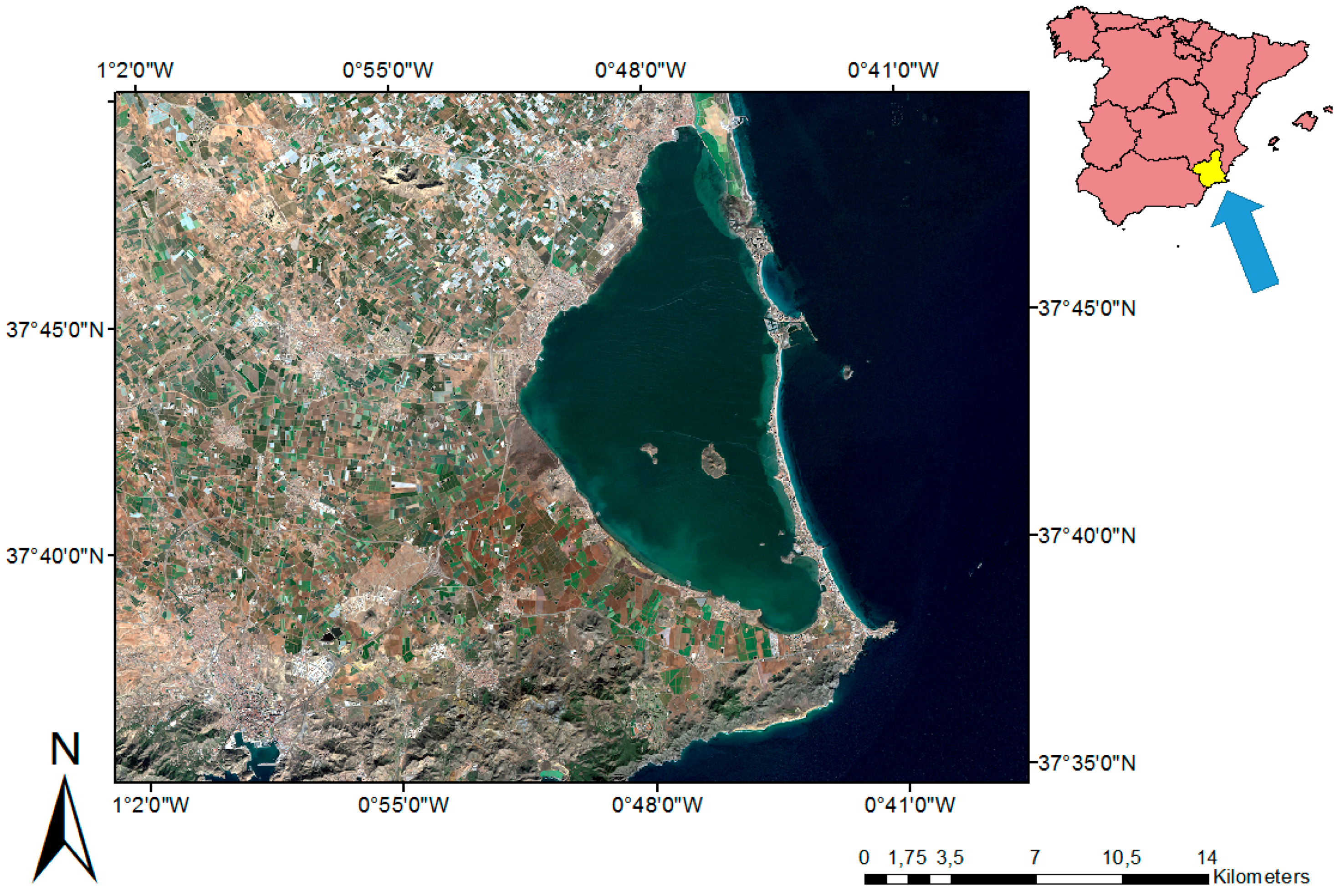
The study area is located in the SE of Spain, in the region of Murcia (Figure 1). These area supports intensive agriculture and big tourist resorts. The studied area is a homogeneous plain slightly inclined towards the coast with a height oscillating from 150–0 m, flanked by a mountainous alignment open to the west with NE-SW direction and a surface area of about 500 km2. The height of the reliefs in the basin is variable, reaching up to 900 m at some interior points. The Menor Sea is a hypersaline lagoon of 135 km2 that is separated from the Mediterranean by a 22 km long barrier beach named “La Manga” crossed by a few shallow channels. The maximum depth of the lagoon is between 6 and 7 m, while the mean is about 3.5 m. Water temperature ranges from 31 °C in Summer to 10 °C in Winter. According to Köppen classification, it is within the dry climate type BWh with a low rate of precipitation (113–498 mm/year).
Geologically, the sedimentary basin of the Menor Sea (Figure 2) consists of Neogene and quaternary materials that lie on the basement of the betic units. To the South, there are parallel elevations to the coast with generalized arrangements East to West, and significant fracturing where the oldest materials emerge. Formations of micaschists and quartzite are Cambrian-Permian. Also present is the Complex Alpujarroide, formed by phyllites and quartzites of the Middle Triassic and carbonate rocks like limestone and Dolomites of the Upper Triassic. The conglomerates, sands, marls and silts correspond to marine transition facies by sea level rise during the Tortonian. Conglomerates and calcarenites, marls in the northern mountain ranges and punctually in the south, and some volcanic islands (of the Miocene-Pliocene boundary) are of the Mesiniense. Disposed sandstones and marls of coastal environments and the bottom of the Pliocene lower basin are in contact with the Mesinian materials of the north. The filling of the basin by these marine-continental transition environments of sands, silts and clays occurred during the Pleistocene itself. During the Holocene, the abrupt oscillations of the sea ceased and there was sedimentation of gravels, sands, silts, and clays by fluvial systems. There is also presence of salt and silt sedimentation in certain endorheic zones. Silt, clays and sands are limited to coastal areas, resulting from the redistribution of coastal drift, waves, tides and winds.
From a geomorphological perspective, the coast of the Menor Sea consists of three large units: mountainous reliefs, a sedimentary basin of filling and a coastal plain that results from coastal dynamics. The mountain reliefs flank the filling basin both north and south of the study area and they are the main source areas of sediment. Their dismantling leads to a large number of surface formations. The erosive action of torrents and streams flowing in favor of the slope gives rise to small alluvial fans and valleys in V, depositing fluvial materials. The location of small glacis evidences a decrease of the slope of the mountainous relief and the change to the second unit, the basin of filling. With a low slope (0–2%), this area is characterized by the presence of alluvial deposits—mainly alluvial fans but also small valley bottoms and some channels that drain into the sea in times of torrential rains.
The third unit has been shaped by the coastal dynamics due to wind, waves and tides, with the barrier island called Manga being the most important geomorphological element since it influences the existence of the Menor Sea. The coastal drift influences this coastal sandy cord with several dune strands formed during the Pleistocene in this zone of the Mediterranean, this being one of the few that still exists. The rest would be submerged by the subsistence character of the region over time.
2.2. Vulnerability Analysis
2.2.1. Remote Sensing Applied in the Delimitation of Exposed Areas
Land cover mapping is one of the main current applications of Remote Sensing [25], which is capable of assisting in the processes of planning and management of natural resources. It is also essential for the study of the main challenges of the environment at the current time, such as climate change, biodiversity, and the demand for agricultural and non-agricultural land uses in the face of world population growth. Of the different classification techniques that have been developed in the last decades, in the present work we have used the classification supervised by the maximum likelihood method [26,27].
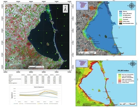
From the two satellite images (Figure 3) SENTINEL2A (MSI); dated 8 July 2017, and Landsat 8 (OLI) (Path: 199, Row: 34); acquisition date 27 July 2017, digital processing is performed using the Geographic Information System (GIS) software ArcGis v10.5. Enhancement of the color composition 6/5/4 (spatial resolution 30 m) is achieved by equalizing the histogram, in order to improve the visual quality of the image. Fusion with the panchromatic band (band 8 with 15 m spatial resolution) was then carried out. The 8/4/3 bands of the SENTINEL-2 satellite (spatial resolution 10 m) were also used to perform a classification supervised by the maximum likelihood method. In the obtained image a low pass filter: mayority filter has been applied with the double objective of softening the spatial contrasts of the image and eliminating the noise of the image. A Kappa index of 0.71 was obtained, considered a “substantial” degree of success, applying a training percentage of 40%, with the rest remaining as validation.
2.2.2. Coastal Vulnerability Index
The present study aims to develop a Coastal Vulnerability Index (CVI) to assess the risk of flooding of the Menor Sea area using 10 related parameters.
In order to do that, we used a derived approach of the Coastal Vulnerability Index (CVI) developed by the United States Geological Survey (USGS) [28]. This CVI method has six physical variables to highlight in a qualitative manner those coastal regions more sensitive to a sea level rise. Prior studies such as [28] have used the USGS-CVI index to carry out similar surveys on the South Coast of Spain, what indicates its suitability to our study area too. Our approach (IVLM) aims to introduce new parameters to improve the adaptability of the assessment to our local conditions as described in Equation (1). Lithology (Fl), land height (Fa), bathymetry (Fb) and the distance between the current coast line to the 10 m high level curve (Fb) have been introduced to better account for coastal vulnerability in the study area [29], while other factors such as geomorphology (Fg), slope (Fp), coast line change rate (Fc), swell factor (Fo), Sea Level Factor (Fnm) and Tidal Range (Frm) have been kept from the USGS-CVI index with slight changes as detailed below:
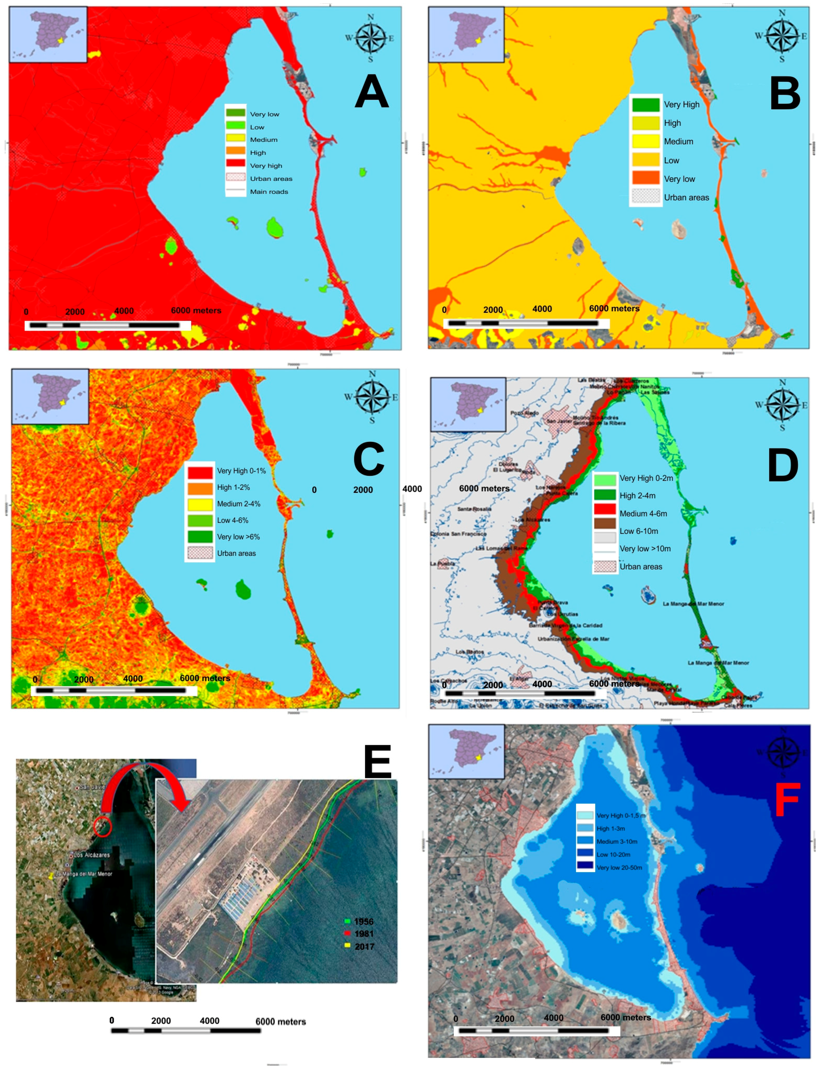
Lithological Factor (Fl). It provides information about the resistance of the rocks against the action of the sea, generating an erosive resistance indicator (Figure 4A). It is obtained by reclassifying the different lithological units according to their hardness to the advance of the water level [21,29].
Geomorphological Factor (Fg). The arrangement of the geomorphological units and associated surface formations (Figure 4B) allows us, depending on the forms and type of deposits, to establish resistances based on their composition and the degree of cementing for the different materials. Furthermore, it accounts for the consistency versus the alterability in case of being located at the seabed. It shows the disaggregation degree of each formation [21,29].
Slope Factor (Fp). The inclination of the terrain (Figure 4C) will influence the advance of the sea inland, either in an eventual form (tsunamis-temporal) or permanently. It also indicates the speed of water retreat in case of a flash flood event. The lower the slope is; the retreat velocity should be higher as the water penetrates more easily into the ground [24].
Height Factor (Fa). It (Figure 4D) is one of the most important to assess the rise of the sea level. We settled the height of 10 m as unattainable figure for a period of 100 years according to estimations based on current trends. Terrain points over 10 m high will therefore be assigned a very low values for this factor, with higher values for those near to the current mean sea level [21,29].
Distance Factor (Fd). Closely related to the height and slope, the distance factor indicates the existing length between the coastline and the 10-m height threshold, which was determined by means of digital processing of the Digital Terrain Model (spatial resolution 5 m). It represents the capacity of the water to advance inland. It has been computed using an extension of the ESRI ArcGis software, created by the USGS Digital Shoreline Analysis System (SDAS) (Figure 4E). Thus, linear distances between the 10-m level curve and the current coastline have been calculated. Then, we created a raster layer based on the standard deviation of the distances to better identify advances or retreats of the coastline [20].
Bathymetry Factor (Fb). It is an important parameter to understand wave dynamics (Figure 4F). Sea waves change their morphology up to a critical point when the distance to the seabed is equal to half the wavelength of the wave front. The friction with the bottom destabilizes the wave and it breaks. Having no data on the wave fronts, this factor gives us information about the effect that the cord may have to stop the thrust of the waves. At low depths, the bathymetric index will be high since it is conditional on the rupture of the wave [30].
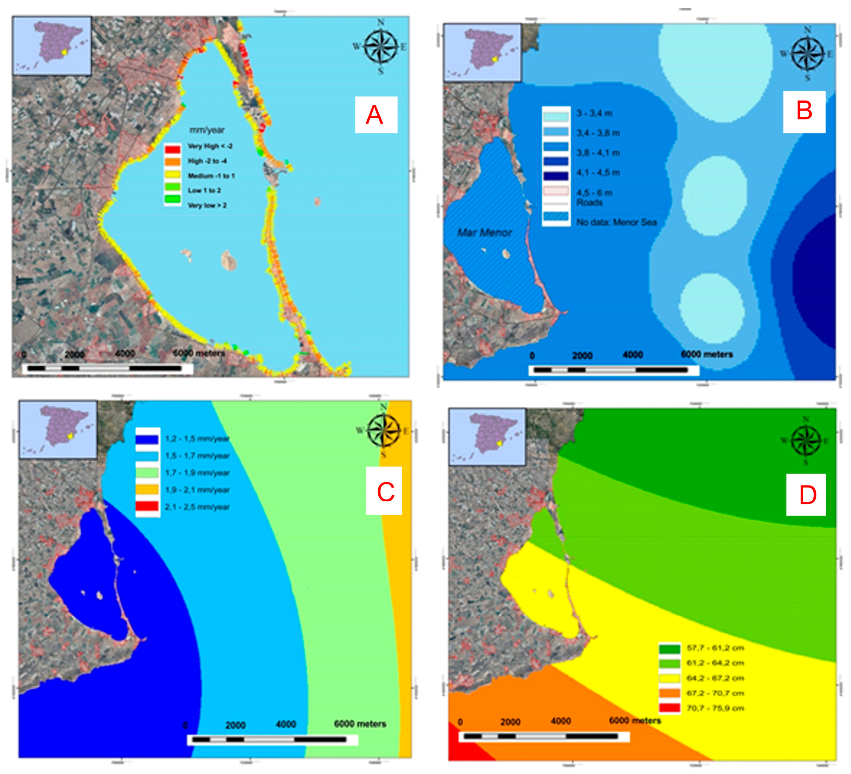
Coastal Factor/West Coast Line Change Rate (Fc). This information was compiled from the viewer of the region of Murcia (Cartomur) and the National Geographic Institute of Spain (IGN). Firstly, we used the aerial photography of 1956 (American Flight) with one-meter resolution, in grayscale. It corresponds to the mosaic of orthophotos of the cartographic service of Murcia region as a result of scanning, digitization, orthorectification and radiometric treatment of the frames that the geographic center of the army had in its photographic archive. Second, the aerial photography of 1981 of the Region of Murcia and thirdly, the ortophoto from PNOA (Plan Nacional de Ortofotografia Aerea) at 0.5 m resolution. This information has been digitized and treated with the USGS DSAS extension for the ArcGis factor (Figure 5A). The 2017 coastline has been taken as a reference to assess its temporal evolution (both regression and accretion). High growth rates corresponds to high vulnerability values, while negative growth rates with low values [20].
Swell Factor: Average Rate of Significant Waves (Fo). The wave factor (Figure 5B) is determined by the maximum values of average significant wave rates that affect the coastal shoreline of the Menor Sea. These data have been obtained from the public agency State Ports, under the Ministry of Development. Data from REDCOS (a network of coastal buoys characterized by being located less than 100 m deep and in the vicinity of port facilities) have been collected from WANA (data simulated from time series of wind and wave parameters), SIMAR 44 (simulated data of time series of atmospheric and oceanographic parameters) and REDEXT (a deep-water buoy network anchored at more than 200 m depth). Wave rates have been interpolated with the mean significant wave rather than the extreme because it encompasses swell states with the highest probability of occurrence. The higher the waves, the higher is the assigned weighted value, since the incidence on the coast would be greater, with very high waves between three and five meters for the coast of the Mediterranean Sea.
Sea Level Factor (Fnm). It determines the relative change of the sea level from the available data of the Menor Sea factor (Figure 5C). There are two potential data sources. The first is the tide gauge network and continual assessment of the mean sea level. The second is the Permanent Service for Mean Sea Level (PSMSL), an organization based in Liverpool that collects, analyzes, interprets, and publishes data related to changes in the global marine level, collected by tide gauges. A linear interpolation was carried out from the information of the tide gauges of Almería, Cartagena, Alicante, and Formentera. For each time series, an average value of the sea level oscillations has been obtained, which has been divided by the number of years to provide a rate for each tide gauge. Interpolating these data, it gives a value for each specific point on the coast. The mean sea level rise rate for the study area is between 1.2 and 1.5 mm/year.
Factor Tidal Range Extreme (Frm). The tidal range is the length difference reached by the water between the high and low tide factor (Figure 4D). Depending on geographical location and local conditions, it varies from a few centimeters to several meters. When the ascent-descent tide difference is less than 2 m, it is considered micro-mareal [25]. The oscillations of the tidal range are obtained from the tide gauges of Almería, Formentera and Gandía. Subsequently, a linear interpolation with this data has been carried out to obtain representative values, as well as to be able to catalog classified values. The maximum tidal ranges recorded for the representative time series have been taken as we are analyzing the risk of coastal flooding. The tidal range for the study area is low, with values of 50–100 cm [25].
2.3. Calculation of the Risk of Flooding of the Menor Sea
In order to calculate the risk of flooding in our study area, we have generated different scenarios of the rise and fall of the sea level based on various time periods: 100 years starting from the present, s. XXI (21st century), 500 years from the present, and 1000 years from the present. In addition, we have considered a scenario of extreme events such as storms or tsunamis based on historical data and supported by sedimentary records close to the study area.
As detailed on the introduction, sea level rise may be accounted for several environmental factors and their impact might vary depending on the time covered by each scenario. We have assumed that parameters such as the extreme mareal range or swell factor will remain constant for the time covered by every scenario with the exception of the extreme events scenario, ranging from the minimum and maximum expected values. Whereas we presume that other factors such as the sea level and neotectonic factors do vary in time. Table 1 summarizes the minimum and maximum expected increase for each scenario, as well as it details which parameters have influence on the sea level rise. We have generated six different scenarios:
Scenario X0A (current): It is based on the wave, tidal range and sea level parameters under analysis on the vulnerability Section 2.2. We have established maximum and minimum ascend rates (mm/year) based on the previous 25 years of tide gauge records (Table 1).
Scenario X1A (T = 100 years and the Neotectonic Factor). The flood risk is estimated for a period of 100 years. The wave and tidal range parameters remain constant, while the sea level rise have the same rate (mm/year) than X0 scenario. In addition, the Neotectonic Factor (subsidence in coastal blocks) is estimated to influence between +4 cm and +7 cm in 1000 years [30], which implies a sinking of the block and consequently an increase of the water sheet with respect to the continental surface (Figure 6).
Scenario X1B (21st Century according to EEA). In this scenario, the swell and tidal range factors obtained from the previous vulnerability analysis are maintained, whereas we use the European Environmental Agency (EEA) prediction of sea level rise for the 21st century in the Mediterranean. This methodology provides data that is somewhat higher than the previous scenario (X1A).
Scenario X2 (T = 500 years: 2012–2512). This scenario involves estimation of the sea level rise over 500 years, and it is based on the predictions of the X1A scenario. It is assumed that the variables of swell and tidal range are stable. The values obtained in the X1A scenario have been extrapolated for a period of 500 years (Figure 6).
Scenario X3 (1000 years). Likewise in the 500-year scenario, the wave and tidal range variables are considered constant, and the X₁A scenario forecast is assumed to be valid for sea level rise (Figure 6).
Scenario with Extreme Events: Storms and Tsunamis. (Figure 7) The Mediterranean area is the collision zone between the European and African plate, which creates volcanic and seismic phenomena that can cause tsunamis. It is a tectonically active zone where the basin depth acts as enhancement. Maximum depths of 3000 m are reached by the Tyrrhenian Sea, while depths of 4000–5000 m are found in the Jonic area [31,32,33]. Ten percent of all tsunamis occur in the Mediterranean, where 7% of earthquakes cause tsunamis. The response time for this type of events are reduced due to the small dimensions of the Mediterranean basin.
Data records from quaternary sedimentary series evidence events that increased the sea water level up to 8 m for the years 1790 and 1829 in Murcia and Conil (Cadiz) [24]. For extreme storm events, there is abundant evidence in the fossil record on the Mediterranean coast—even in sectors close to the study area—specifically in the provinces of Murcia, Almeria and Alicante [31]. These records that are whether erosive or depositional, show a rise in sea level under stormy conditions up to two meters [34,35]. The chronological sequence of events does not indicate cyclicity but it is possible to know the relative ages of such catastrophic events: 365 A.C.; 1680; 1804; 1860 and 1875 [32,34].
By means of historical records, we know that there have not been giant waves in the Mediterranean basin such as it occurs in higher latitudes with tropical storms. Even in weather events like tropical cyclones, the waves would not have reached the height nor the time span they take in the oceans. The decrease in number and frequency of meteorological events (storms) in the Mediterranean Sea is foreseeable [35], but it is necessary to consider their current existence and incidence on the coast of the Menor Sea.
3. Results and Discussion
3.1. Coastal Vulnerability in the Menor Sea
In the first phase, analysis by means of Remote Sensing techniques from images provided by Landsat 8 and SENTINEL-2 allowed us to establish the locations of the different human activities in the sectors that surround the Menor Sea. Before conducting a supervised classification of a satellite image, it is necessary to study the actual separability of the selected categories, so that they can be classified without risk of confusion. For this reason, a table and a graph (Figure 8) were drawn with the spectral curves of the different land covers, in which the bands involved in the analysis appear on the abscissa axis and the average Digital Levels of each category on the axis of ordinates. This graph is very useful for an initial assessment of the spectral trends of each category. In addition, it identifies those spectral bands in which a peculiar behavior manifests with respect to the neighboring classes. The parallel and near lines indicate a likely overlap between categories, while intersections between lines manifest in bands where they are most likely to separate the categories they represent. According to this criterion we have chosen bands 6, 5 and 4 to perform the supervised classification of the image acquired by the Landsat 8 satellite. Figure 8 shows the fusion of the panchromatic channel (band 8) with the color composition 6/5/4 of the satellite image (Landsat 8). The main objective of this fusion technique is to enhance the visual aspect of the image (composition 6/5/4), with a spatial resolution of 30 m, using information provided by a better spatial resolution (band 8) with a resolution of 15 m. The end result is that an image containing the chromatic detail of the 6/5/4 bands and the spatial quality of the band 8 has been obtained. This procedure has been applied by the Gram-Schmidt pan-sharpening method is based on a general algorithm for vector orthogonalization—the Gram-Schmidt orthogonalization.
To carry out the supervised classification, six types of decks have been defined (water, crops, greenhouses, bare soils, urban hulls, and natural vegetation). These classes represent the dominant and most important decks of the studied area. In each of the classes, sufficiently representative areas (training fields) have been delimited in order to obtain precise recognition and to differentiate the different categories. For a more precise location of the training areas, previous field work, aerial photography, and land use map have proven to be very helpful.
They have been selected on the order of about 100 pixels, scattered in the image, for each cover. In the more heterogeneous class such as the urban helmets, with the presence of houses, streets, gardens, etc., larger pixels have been chosen in order to acquire an average signal of the different components and avoid the more intense border effects, as usually happens when choosing smaller pixels. The cover constituted by plastic greenhouses offers the most peculiar behavior, with the highest values of the Digital Levels in all the studied bands. The crops offer a clear diversity because their contrast between bands 4, 5, 6 and 7 is large. Bare soils have the highest values in bands 5 and 6, while urban and natural vegetation show similar behavior in all bands, although with different degrees of reflectivity, being lower in the case of natural vegetation. The water shows the lowest values of reflectivity because it absorbs most of the incidental energy, and even more so at larger wavelengths.
In the second phase, the vulnerability has been calculated from a modified USGS Coastal Vulnerability Index (CVI) which has been used in similar studies [21,29]. The IVLM index has made possible to establish the vulnerability of the Menor Sea area, both for predictable sea level rise and for stormy events or tsunamis. By means of map algebra we have crossed the different factors contained in the index, obtaining a map (Figure 9) that spatially represents the degree of vulnerability (ranging from one to five). The greater the value of the index, the greater will be its vulnerability to the rise of the water sheet. Each individual factor described in Section 2.2.2 has got its relative importance in the final outcome of the index. Lithology and geomorphology are closely linked with the resistance of the materials, their permeability, texture or alterability [36]. The elevation of the terrain slope and distance factors play a fundamental role as obstacles to the water advance [37], while the coastal factor provides an insight about the evolution trend of the coast line as well as helping to identify coastal hazards [38]. Bathymetry affects the behavior of the waves and as [39] explains, this kind of data helps to improve the coastal management. Swell, sea level and tidal range features the regional behavior of the Mediterranean Sea, what permits that our index fits better than broader vulnerability analysis over at larger scales [40].
The results indicate a high flooding risk with any sea level increase, at least for the coast and barrier beach of the Menor Sea. These are heavily urbanized areas with high vulnerability due to the characteristics of the physical environment. Vulnerability values range from high to very high for the west coast of the Menor Sea, as well as for specific stretches of the “Manga” (barrier beach) that alternate with medium and low values. Low or very low values are concentrated a few hundred meters away from the coast line. Particular populations such as the south of San Pedro del Pinatar, Santiago de la Ribera (Pedanía de San Javier), part of the airport of San Javier, Los Alcázares, Playa Honda, and some of the hotel complexes and urbanizations of the south and center of the Manga, are very vulnerable according to the applied coastal index. The reason to create new parameters, such as the bathymetric or the geomorphological ones, was in order to improve the accuracy of the evaluation.
3.2. Risk of Flooding in the Menor Sea
Taking into account the different scenarios, it has been observed that the most densely populated places certainly coincide with those that present the highest risk, since many of them are below eight meters in height. The barrier beach of the Menor Sea is especially susceptible, with values between zero and two meters. The scenarios of 500 and 1000 years show much greater uncertainty since the weather patterns are constantly changing, furthermore over longer periods of time when this change is even more pronounced [28].
In the short term, storm surge events are the most important and likely risks to occur since a flood over inhabited areas can cause suddenly serious human and economic damages. Hotel complexes and urbanizations situated only a few meters from the beach are very exposed to sudden events of this nature and the capacity to react is very limited. This is not the case for the estimated 100-year rise (scenario X1A) or for the 21st century (scenario X1B) since the expectancy of water level increase is slower and some land management measures may be carried out in advance to prevent damages. The Menor Sea as we know it today would disappear, leaving only two zones remaining, in the form of islands. The maximum expected rise for the X1B scenario is somewhat more ambitious than for the X1A scenario, which would imply a larger flooded area. It should be noted that in Figure 10 the X1B scenario has not been represented for reasons of graphic overlap in order to maintain quality in the image.
The short time series available from tide gauges and buoys, coupled with the continuous change of estimated trends for this century, makes this topic very controversial. The broad spectrum of future predictions [41,42], coupled with the uncertainty of the past (old tide records since 1880) leave fossil sedimentary records as one of the few witnesses to sea level change stepping back more than 50 years, which on the other hand it is quite inaccurate both temporally and spatially. Nevertheless, data records from the recent past may help us to identify reliable patterns that can be repeated in the near future, and (Table 2) indicates the contribution observed since 1972 at global scale.
Based on the 25 year record of the mean sea level for our study area, we obtained a mean rate between 1.2 and 1.5 mm/year. These rates are lower than those observed for the gauges in Table 2, what confirms that local factors play a fundamental role in the behavior of the sea level. Previous forecasts of sea level rise at global scale have not taken into account the wave, tidal range, or neotectonic factor. This invalidates, to a certain extent, a direct transposition of these values over a specific area while giving greater reliability to local studies where flood risks are addressed and evaluated against the worst simulated rise scenario. Bearing in mind those factors in our study, the shortest case scenarios (X1A and X1B) estimates and increase of the water sheet in the Mediterranean from +4.53 to +4.92 m and +4.22 to +5.69 m respectively in 100 years, although we may expect some uncertainty in our predictions.
Ascent forecasts are subjected to climate models, which tend to predict future wind patterns, changes in solar activity, temperatures or rainfall. However, future estimates are very risky over long time periods, presenting some uncertainties in their models [43] since they are subjected to continuous natural changes. Furthermore, they can be altered by human factors (conflict over the contribution of human activities to climate change) [44], invalidating or modifying any prediction that goes beyond a few decades onwards. They are therefore purely hypotheses with model uncertainties that we have attempted to solve using in situ data of the zone. Even though barrier beaches as other geomorphological units may reduce the effect of tsunami waves of low intensity, we have not factored this parameter in our model. We aimed to state the worst case scenario and based on certain historical records, there have been tsunamis that increased the water level up to 8 m, which is higher than the mean height of “La Manga” barrier beach. As stated by [45], narrow barrier beaches and absorbers cannot stop high intensity tsunamis. More abundant and reliable historical records will improve further modelizations.
3.3. Environmental Impacts
The Corine Land Cover provides valuable information on categorizing the level of damage caused by flooding in the study area (Figure 11). Based on Corine 2006, a land use reclassification has been made based on human factors. Urban and industrial zones have been assigned with a high value, where most of the population is symbolized by the color red. For average values, we would have those places of human transit, where there is not always activity; crops, roads, forests, harbors, heaps, beaches, etc.
Finally, a low value is given to areas with infrequent human presence; for example, wetlands, saltworks, rocks, pastures, and sclerophyllous scrubs. Loss of land, classified with an impact index 3 (high human presence), is quite important, affecting a large part of the coastal area of the Menor Sea and Mediterranean. Under any flood scenario, these areas are seriously threatened. The index for the rest of the land, consists of irrigated agricultural land, fruit trees, beaches, and intertidal plains is mostly medium. Low values are practically non-existent, except for specific cases of near-shore wetlands.
4. Conclusions
The procedure used in this work allows the accurate and effective delimiting of the coastal areas with risk of flooding due to sea level rise, at a low economic cost at early stages of coastal planning. The degree of vulnerability and flood risk that is presented by the Menor Sea before a rise of the sea level, if it is generated by a progressive rise or by extreme events, is determined.
The methodology is validated by matching the affected areas of the vulnerability method (based on empirical methods of the parameters of the study area) to the risk method (based on deterministic methods using time trend scenarios). Many forecasts on the quantification of sea level rise on a global scale do not take into account the swell factor and tidal range, which at some extent invalidates a direct transposition of those values over a particular area. This gives greater weight to the reliability of local studies, where flood risks are addressed and evaluated against the worst simulated scenario of sea level rise. Finally, this cartography is a preventive measure to minimize the risk on this coast, which has large urbanizations and tourist complexes, and it receives large numbers of tourists from all over the world. This tool can establish the sectors that need structural measures to minimize the impact of sea level rise occurring due to natural tendency, or extreme events in the short and long term. These are areas with a high vulnerability due to the characteristics of the physical environment and a high risk of flood due to their geographical position.
Acknowledgments
This research was funded by projects from the Ministry of Economy and Competitiveness CGL2015-67169-P and CGL2015-69919-R.
Author Contributions
For research articles presented in this paper is a collaborative development by all authors. All the authors analyzed the risk of coastal flooding and the involved parameters Diego Gómez, Antonio Miguel Martinez-Graña and Fernando Santos-Francés analyzed the treatment and reclassification of the satellite images by techniques of remote sensing with ArcGis. The manuscript was written, revised, and corrected by all co-authors.
Conflicts of Interest
The authors declare no conflict of interest.
References
- Stenseth, N.C.; Ottersen, G.; Hurrell, J.W.; Mysterud, A.; Lima, M.; Chan, K.S.; Yoccoz, N.G.; Ådlandsvik, B. Studying climate effects on ecology through the use of climate indices: The North Atlantic Oscillation, El Nino Southern Oscillation and beyond. Proc. R. Soc. Lond. B Biol. Sci. 2003, 270, 2087–2096. [Google Scholar] [CrossRef] [PubMed]
- Klein Tank, A.M.G.; Wijngaard, J.B.; Können, G.P.; Böhm, R.; Demarée, G.; Gocheva, A.; Milrta, M.; Pashiardis, S.; Hejkrlik, L.; Heino, R.; et al. Daily dataset of 20th-century surface air temperature and precipitation series for the European Climate Assessment. Int. J. Climatol. 2002, 22, 1441–1453. [Google Scholar] [CrossRef]
- Karl, T.R.; Trenberth, K.E. Modern global climate change. Science 2003, 302, 1719–1723. [Google Scholar] [CrossRef] [PubMed]
- Vitousek, P.M. Beyond global warming: Ecology and global change. Ecology 1994, 75, 1861–1876. [Google Scholar] [CrossRef]
- Kirschbaum, M.U. The temperature dependence of soil organic matter decomposition, and the effect of global warming on soil organic C storage. Soil Biol. Biochem. 1995, 27, 753–760. [Google Scholar] [CrossRef]
- Mori, N.; Yasuda, T.; Mase, H.; Tom, T.; Oku, Y. Projection of extreme wave climate change under global warming. Hydrol. Res. Lett. 2010, 4, 15–19. [Google Scholar] [CrossRef]
- Trenberth, K.E. Changes in precipitation with climate change. Clim. Res. 2011, 47, 123–138. [Google Scholar] [CrossRef]
- Rahmstorf, S. A semi-empirical approach to projecting future sea-level rise. Science 2007, 315, 368–370. [Google Scholar] [CrossRef] [PubMed]
- Church, J.A.; Clark, P.U.; Cazenave, A.; Gregory, J.M.; Jevrejeva, S.; Levermann, A.; Merrifield, M.A.; Milne, G.A.; Nerem, R.S.; Nunn, P.D.; et al. Sea Level Change. In Climate Change 2013: The Physical Science Basis. Contribution of Working Group I to the Fifth Assessment Report of the Intergovernmental Panel on Climate Change; Cambridge University Press: Cambridge, UK; New York, NY, USA, 2013. [Google Scholar]
- Meehl, G.A. Global climate projections. In Climate Change 2007: The Physical Science Basis. Contribution of Working Group I to the Fourth Assessment Report of the Intergovernmental Panel on Climate Change; Solomon, S., Qin, D., Manning, M., Chen, Z., Marquis, M., Averyt, K.B., Tignor, M., Miller, H.L., Eds.; Cambridge University Press: Cambridge, UK; New York, NY, USA, 2007; pp. 755–828. [Google Scholar]
- Bindoff, N.L.; Willebrand, J.; Artale, V.; Cazenave, A.; Gregory, J.; Gulev, S.; Hanawa, K.; Le Quéré, C.; Levitus, S.; Nojiri, Y.; et al. Observations: Oceanic Climate Change and Sea Level. In Climate Change 2007: The Physical Science Basis. Contribution of Working Group I to the Fourth Assessment Report of the Intergovernmental Panel on Climate Change; Solomon, S., Qin, D., Manning, M., Chen, Z., Marquis, M., Averyt, K.B., Tignor, M., Miller, H.L., Eds.; Cambridge University Press: Cambridge, UK; New York, NY, USA, 2007. [Google Scholar]
- Bardají, T.; Zazo, C.; Cabero, A.; Dabrio, C.; Goy, J.L.; Lario, J.; Silva, P.G. Impacto del Cambio Climático en el litoral. Enseñanza de las Ciencias de la Tierra 2009, 17, 141–154. [Google Scholar]
- Vellinga, M.; Wood, R. Impacts of thermohaline circulation shutdown in the twenty-first century. Clim. Chang. 2008, 91, 43–63. [Google Scholar] [CrossRef]
- Pfeffer, W.T.; Harper, J.T.; O’Neel, S. Kinematic constraints on glacier contributions to 21st-century sea-level rise. Science 2008, 321, 1340–1343. [Google Scholar] [CrossRef] [PubMed]
- Kopp, R.E.; Simons, F.J.; Mitrovica, J.X.; Maloof, A.C.; Oppenheimer, M. Probabilistic assessment of sea level during the last interglacial stage. Nature 2009, 462, 863–868. [Google Scholar] [CrossRef] [PubMed]
- Vermeer, M.; Rahmstorf, S. Global sea level linked to global temperature. Proc. Natl. Acad. Sci. USA 2009, 106, 21527–21532. [Google Scholar] [CrossRef] [PubMed]
- Grinsted, A.; Moore, J.C.; Jevrejeva, S. Reconstructing sea level from paleo and projected temperatures 200 to 2100 AD. Clim. Dyn. 2010, 34, 461–472. [Google Scholar] [CrossRef]
- Katsman, C.A.; Oldenborgh, J.V. Exploring high-end scenarios for local sea level rise to develop flood protection strategies for a low-lying delta—The Netherlands as an example. Clim. Dyn. 2011, 109, 617–645. [Google Scholar] [CrossRef]
- Intergovernmental Panel on Climate Change (IPCC). Climate Change 2014: Synthesis Report. Contribution of Working Groups I, II and III to the Fifth Assessment Report of the Intergovernmental Panel on Climate Change; IPCC: Geneva, Switzerland, 2014. [Google Scholar]
- Thieler, E.R.; Himmelstoss, E.A.; Zichichi, J.L.; Ergul, A. Digital Shoreline Analysis System (DSAS) Version 4.3—An ArcGIS Extension for Calculating Shoreline Change; U.S. Geological Survey Open-File Report 2008-1278; U.S. Geological Survey: Reston, VA, USA, 2009.
- Ojeda, J.; Álvarez, J.I.; Martín, D.; Fraile, P. El uso de las TIG para el cálculo del índice de vulnerabilidad costera (CVI) ante una potencial subida del nivel del mar en la costa andaluza. España. Rev. Int. Cienc. Tecnol. Inf. Geogr. 2009, 9, 83–100. [Google Scholar]
- De Pascalis, F.; Pérez-Ruzafa, A.; Gilabert, J.; Marcos, C.; Umgiesser, G. Climate change response of the Mar Menor coastal lagoon (Spain) using a hydrodynamic finite element model. Estuar. Coast. Shelf Sci. 2012, 114, 118–129. [Google Scholar] [CrossRef]
- Pérez-Ruzafa, A.; Marcos, C.; Pérez-Ruzafa, I.M.; Ros, J. Evolución de las Características Ambientales y de los Poblamientos del Mar Menor (Murcia, SE de España). In Anales de Biología. 1987, pp. 53–65. Available online: http://revistas.um.es/analesbio/article/view/35381 (accessed on 12 March 2018).
- Pilkey, O.H.; Davis, T.W. An analysis of coastal recession models North Carolina coast. Sea level fluctuation and coastal evolution: Tulsa, Okla. Soc. Econ. Paleontol. Mineral. 1987, 41, 59–68. [Google Scholar]
- Masselink, G.; Short, A.D. The effect of tidal range on beach morphodynamics and morphology: A conceptual beach model. J. Coast. Res. 1993, 9, 785–800. [Google Scholar]
- Chuvieco, E. Teledetección Ambiental. La Observación de la Tierra Desde el Espacio; Ariel: Barcelona, Spain, 2008. [Google Scholar]
- Tso, B.; Mather, P. Classification Methods for Remotely Sensed Data; CRC Press Taylor & Francis Group: Boca Raton, FL, USA, 2009. [Google Scholar]
- Hallegatte, S. Strategies to adapt to an uncertain climate change. Glob. Environ. Chang. 2009, 19, 240–247. [Google Scholar] [CrossRef]
- Martínez-Graña, A.M.; Boski, T.; Goy, J.L.; Zazo, C.; Dabrio, C.J. Coastal-flood risk management in Central Algarve: Vulnerability and Flood Risk Indices (South Portugal). Ecol. Indic. 2016, 71, 302–316. [Google Scholar] [CrossRef]
- Somoza, L. Estudio del Cuaternario Litoral Entre Cabo de Palos y Guardamar (Murcia-Alicante). Las Variaciones del Nivel del Mar en Relación con el Contexto Geodinámico; Spanish Institute of Oceanography: Barcelona, Spain, 1993; Volume 12. [Google Scholar]
- Lario, J.; Luque, L.; Zazo, C.; Goy, J.L.; Spencer, C.; Cabero, A.; Bardají, T.; Borja, F.; Dabrio, C.J.; Civis, C.; et al. Tsunami vs. storm surge deposits: A review of the sedimentological and geomorphological record of Extreme Waves Events (EWE) during the Holocene in the Gulf of Cadiz, Spain”. Z. Geomorphol. 2010, 54 (Suppl. 3), 231–235. [Google Scholar] [CrossRef]
- Lario, J.; Zazo, C.; Goy, J.L.; Silva, P.G.; Bardají, T.; Cabero, A.; Dabrio, C.J. Holocene paleotsunami catalogue of SW Iberia. Quat. Int. 2011, 242, 196–200. [Google Scholar] [CrossRef] [Green Version]
- Samaras, A.G.; Karambas, T.V.; Archetti, R. Simulation of tsunami generation, propagation and coastal inundation in the Eastern Mediterranean. Ocean Sci. 2015, 11, 643–655. [Google Scholar] [CrossRef]
- Luque, L.; Lario, J.; Zazo, C.; Goy, J.L.; Dabrio, C.J.; Silva, P.G. Tsunami deposits as paleoseismic indicators: Examples from the Spanish coast. Acta Geol. Hisp. 2001, 36, 197–211. [Google Scholar]
- Marcos, M.; Jordà, G.; Gomis, D.; Pérez, B. Changes in storm surges in southern Europe from a regional model under climate change scenarios. Glob. Planet. Chang. 2011, 77, 116–128. [Google Scholar] [CrossRef]
- Forte, F.; Pennetta, L.; Strobl, R.O. Historic records and GIS applications for flood risk analysis in the Salento peninsula (Southern Italy). Nat. Hazards Earth Syst. Sci. 2005, 5, 833–844. [Google Scholar] [CrossRef]
- Kazakis, N.; Kougias, I.; Patsialis, T. Assessment of flood hazard areas at a regional scale using an index-based approach and Analytical Hierarchy Process: Application in Rhodope–Evros region, Greece. Sci. Total Environ. 2015, 538, 555–563. [Google Scholar] [CrossRef] [PubMed]
- Ferreira, O.; Garcia, T.; Matias, A.; Taborda, R.; Dias, J.A. An integrated method for the determination of set-back lines for coastal erosion hazards on sandy shores. Cont. Shelf Res. 2006, 26, 1030–1044. [Google Scholar] [CrossRef]
- Kroon, A.; Davidson, M.A.; Aarninkhof, S.G.J.; Archetti, R.; Armaroli, C.; Gonzalez, M.; Medri, S.; Osorio, A.; Aagaard, T.; Holman, R.A.; et al. Application of remote sensing video systems for coastline management problems. Coast. Eng. 2007, 54, 493–505. [Google Scholar] [CrossRef]
- Cahoon, D.R.; Hensel, P.F.; Spencer, T.; Reed, D.J.; McKee, K.L.; Saintilan, N. Coastal wetland vulnerability to relative sea-level rise: Wetland elevation trends and process controls. In Wetlands and Natural Resource Management; Springer: Berlin/Heidelberg, Germany, 2006; pp. 271–292. [Google Scholar]
- Church, J.A.; White, N.J. Sea-Level Rise from the Late 19th to the Early 21st Century. Surv. Geophys. 2011, 32, 585–602. [Google Scholar] [CrossRef]
- Nicholls, R.; Mimura, N. Regional issues raised by sea-level rise and their policy implications. Clim. Res. 1998, 11, 5–18. [Google Scholar] [CrossRef]
- Hawkins, E.; Sutton, R. The potential to narrow uncertainty in regional climate predictions. Bull. Am. Meteorol. Soc. 2009, 90, 1095–1107. [Google Scholar] [CrossRef]
- Oreskes, N. The scientific consensus on climate change. Science 2004, 306, 1686. [Google Scholar] [CrossRef] [PubMed]
- Shukla, S.B.; Prizomwala, S.P.; Ukey, V.; Bhatt, N.; Chamyal, L.S. Coastal geomorphology and tsunami hazard scenario along the Kachchh Coast, Western India. Indian J. Geo-Mar. Sci. 2010, 39, 549–556. [Google Scholar]
Figure 1.
Location of the study area: Menor Sea in Murcia (Spain). RGB composite of a Sentinel 2B image (16 January 2018), surface reflectance (BOA) corrected product with 10 m spatial resolution.
Figure 1.
Location of the study area: Menor Sea in Murcia (Spain). RGB composite of a Sentinel 2B image (16 January 2018), surface reflectance (BOA) corrected product with 10 m spatial resolution.

Figure 2.
Lithological map (up) and geomorphological map (down).

Figure 3.
(A) Landsat 8 with 6/5/4 color composition enhancement (spatial resolution 30 m); (B) Classification supervised by the maximum likelihood method of the Landsat 8; (C left) SENTINEL-2 8/4/3 band combination (spatial resolution 10 m); (C right) Classification supervised by the maximum likelihood method of the SENTINEL-2.

Figure 4.
(A) Lithological factor map; (B) Geomorphological factor map; (C) Slope factor map; (D) Height factor map; (E) Distance factor map; (F) Bathymetry factor map.
Figure 4.
(A) Lithological factor map; (B) Geomorphological factor map; (C) Slope factor map; (D) Height factor map; (E) Distance factor map; (F) Bathymetry factor map.

Figure 5.
(A) Coastal factor map/west coast line change rate map; (B) Swell factor map/average rate of significant wave map (C). Sea level factor map; (D) Factor tidal range extreme map.
Figure 5.
(A) Coastal factor map/west coast line change rate map; (B) Swell factor map/average rate of significant wave map (C). Sea level factor map; (D) Factor tidal range extreme map.

Figure 6.
Map of maximum expected sea level rise for a scenario of 100 years based on the parameters of the X1A scenario (top left). Map of maximum expected sea level rise for 21st century based on the parameters of scenario X1B (top right). Map of maximum expected sea level rise for the 500-year scenario based on the parameters of the X1A scenario (bottom left). Map of maximum expected sea level rise for the 1000-year scenario based on the parameters of the X1A scenario (bottom right).

Figure 7.
Maximum expected water sheet rise map for extreme weather events: storms (left) and maximum expected water sheet rise map for tsunamis (right).
Figure 7.
Maximum expected water sheet rise map for extreme weather events: storms (left) and maximum expected water sheet rise map for tsunamis (right).

Figure 8.
Fusion of the panchromatic channel (band 8) with the color composition 6/5/4 of the satellite image (Landsat 8 (up) and spectral signatures for different terrain coverages in the study area (down)).
Figure 8.
Fusion of the panchromatic channel (band 8) with the color composition 6/5/4 of the satellite image (Landsat 8 (up) and spectral signatures for different terrain coverages in the study area (down)).

Figure 9.
Mapping of coastal vulnerability in the Menor Sea according to the index IVLM.

Figure 10.
Flood Risk Mapping in the Menor Sea for the various scenarios proposed (except X1B, to promote visibility).
Figure 10.
Flood Risk Mapping in the Menor Sea for the various scenarios proposed (except X1B, to promote visibility).

Figure 11.
Flood Risk Mapping in the Menor Sea for the different scenarios proposed (except for X1B, to guarantee image quality and to avoid overlap) along with land uses (Corine, 2006) grouped according to the indexes indicated above.
Figure 11.
Flood Risk Mapping in the Menor Sea for the different scenarios proposed (except for X1B, to guarantee image quality and to avoid overlap) along with land uses (Corine, 2006) grouped according to the indexes indicated above.


Table 1.
Maximum and minimum expected increases of the water sheet in the different scenarios.
| Minimum Values (m) | Maximum Values (m) | ||||||||||
|---|---|---|---|---|---|---|---|---|---|---|---|
| Scenarios | X0A | X1A | X1B | X2 | X3 | X0A | X1A | X1B | X2 | X3 | Extreme Value |
| Swell | 3.8 | 3.8 | 3.8 | 3.8 | 3.8 | 4.1 | 4.1 | 4.1 | 4.1 | 4.1 | |
| Rise Sea level | 0.03 | 0.12 | −0.19 | 0.6 | 1.2 | 0.0375 | 0.15 | 0.92 | 0.75 | 1.5 | |
| Mareal Range | 0.61 | 0.61 | 0.61 | 0.61 | 0.61 | 0.67 | 0.67 | 0.67 | 0.67 | 0.67 | |
| Neotectonic | 0.00 | 0.00 | 0.00 | 0.02 | 0.04 | 0.00 | 0.00 | 0.00 | 0.03 | 0.07 | |
| Weather Event | 0.00 | 0.00 | 0.00 | 0.02 | 0.04 | 0.00 | 0.00 | 0.00 | 0.03 | 0.07 | +2 m |
| Tsunami | 0.00 | 0.00 | 0.00 | 0.02 | 0.04 | 0.00 | 0.00 | 0.00 | 0.03 | 0.07 | +8 m |
| Total | +4.53 | +4.53 | +4.22 | +5.03 | +5.65 | +4.929 | +4.92 | 5.69 | +5.55 | +6.34 | |
| Component | 1972–2008 (mm/year) | 1993–2008 (mm/year) |
|---|---|---|
| Gauges (Total) | 1.83 ± 0.18 | 2.61 ± 0.55 |
| Gauges and altimeters (Total) | 2.10 ± 0.16 | 3.22 ± 0.41 |
| 1. Thermal expansion | 0.80 ± 0.15 | 0.88 ± 0.33 |
| 2. Glaciers and ice sheets | 0.67 ± 0.03 | 0.99 ± 0.04 |
| 3. Ice of Greenland | 0.12 ± 0.17 | 0.31 ± 0.17 |
| 4. Antarctic ice | 0.30 ± 0.20 | 0.43 ± 0.20 |
| 5. Land storage | −0.11 ± 0.19 | −0.08 ± 0.19 |
| Sum of components (1 + 2 + 3 + 4 + 5) | 1.78 ± 0.36 | 2.54 ± 0.46 |
© 2018 by the authors. Licensee MDPI, Basel, Switzerland. This article is an open access article distributed under the terms and conditions of the Creative Commons Attribution (CC BY) license (http://creativecommons.org/licenses/by/4.0/).
Share and Cite
MDPI and ACS Style
Martínez-Graña, A.; Gómez, D.; Santos-Francés, F.; Bardají, T.; Goy, J.L.; Zazo, C. Analysis of Flood Risk Due to Sea Level Rise in the Menor Sea (Murcia, Spain). Sustainability 2018, 10, 780. https://doi.org/10.3390/su10030780
AMA Style
Martínez-Graña A, Gómez D, Santos-Francés F, Bardají T, Goy JL, Zazo C. Analysis of Flood Risk Due to Sea Level Rise in the Menor Sea (Murcia, Spain). Sustainability. 2018; 10(3):780. https://doi.org/10.3390/su10030780
Chicago/Turabian StyleMartínez-Graña, Antonio, Diego Gómez, Fernando Santos-Francés, Teresa Bardají, José Luis Goy, and Caridad Zazo. 2018. "Analysis of Flood Risk Due to Sea Level Rise in the Menor Sea (Murcia, Spain)" Sustainability 10, no. 3: 780. https://doi.org/10.3390/su10030780
Note that from the first issue of 2016, this journal uses article numbers instead of page numbers. See further details here.