Monitoring and Modelling Bio-Physical Parameters for Hypoxia Hazard in a Coastal Sand Pit

Abstract

Management of coastal areas requires monitoring and modeling of the anthropogenic drivers and the bio-physical processes affecting water quality. To assess the range of hydrographic conditions controlling oxygen distribution in the bottom layers of sand pits, a multi-year oceanographic survey has been conducted in a coastal area with several extraction pits. Hydrographic data including profiles of temperature, salinity and oxygen were collected and related to local wind conditions and circulation. Moreover, 1D and 3D high-resolution non-hydrostatic ocean models were used to describe turbulent mixing regimes and to obtain the range of wind speeds for which the critical anoxic conditions may occur. It is shown that wind speed appears to control the dynamics of oxygen concentrations, with oxygen depleted zones developing in a short time in low wind speed conditions. Moreover, the depth and the shape of the extraction pit contribute to decrease the mixing of the bottom layers and increase the water retention in the hole increasing the output and the persistence of oxygen depleted zones in the excavated area. The results of the numerical simulations show that the risk of hypoxia at the bottom of the sand pits is associated with higher temperatures and wind speed lower than 5 m/s, which is not infrequent during the summer season. However, the number of consecutive days of oxygen depletion can be considered lower than the danger threshold level assumed in the literature.

1. Introduction

The term coastal hypoxia refers to the depletion of oxygen in the bottom waters of coastal systems; this phenomenon occurs when the consumption of oxygen outweighs the oxygen supply for a sufficiently long period [1]. Water masses can become under-saturated with oxygen when organic carbon, produced by photosynthesis and microbial respiration, is aerobically decomposed at a greater rate than that of oxygen re-aeration. In this situation, major impacts may occur to the coastal ecosystems, as, below a certain “hypoxia threshold”, marine organisms are exposed to a variety of stresses, which become lethal when the oxygen concentration becomes too low [2]. Early stages of hypoxia are often missed until obvious signs, such as mass mortality of fish, indicate that thresholds have been passed. Examples can be found in the Gulf of Mexico and the East China Sea, and in European waters, the Adriatic Sea, the German Bight, the Baltic Sea and the north western shelf of the Black Sea [3]. Upwelling of anoxic water in Tokyo Bay, Japan, called blue tide, sometimes causes benthic animal mortality in shallow and tidal flats at the head of the bay [4,5,6].

Intermittent low oxygen conditions affect many of the shallower areas of the Kattegat [7] with the development of severe seasonal hypoxia in the southeastern Kattegat which negatively affects both the benthos and the Norway lobster fisheries [8]. Exposure to low dissolved oxygen concentrations also appears to have an immunosuppression effect. The incidence of diseases such as lymphocystis, epidermial hyperplasias, and papillomas in dab (Limanda limanda) in the eastern North Sea and southern Kattegat increased in the year following hypoxia and remained elevated for 3–4 years at stations experiencing oxygen concentrations <3 mg L⁻¹ [9]. In the inner Danish waters, Behrens et al. [10] estimated how oxygen deficiency may reduce the extent of suitable habitat for sandeels, a small planktivorous fish. They observed that hypoxia normally develops in late summer and early autumn, when warm and calm periods prevail for longer periods. They also underlined that increased temperature would further exacerbate the situation by augmenting sediment oxygen demand. Moreover, Conley et al. [11] demonstrated that the combination of sustained eutrophication with future climate change could intensify hypoxia to new levels of ecosystem impacts.

The amount of oxygen present in waters is normally expressed as a concentration (mg L⁻¹) or as a percentage of full saturation at specific temperature and salinity conditions. The measure of hypoxia effects on organisms is generally evaluated over the period that the dissolved oxygen level is below 2 mg L⁻¹ [12]. In general, percentage saturation is a more useful unit for comparing oxygen values, where there are large seasonal changes in salinity and temperature values. The oxygen re-supply rate is indirectly related to its isolation from the surface layer, which is increased for sand pits excavated by suction dredges for mineral extraction. For this reason, formation of hypoxic areas has been aggravated in Denmark by intensive sand extraction [13].

To assess the sustainability of the dredging activity and the main negative effects induced, monitoring and modeling of bio-physical parameters has to be set up, particularly in waters with high residence times in areas of restricted exchange, which may experience considerable oxygen depletion if oxygen consuming organic matter is present [14]. Aerated oxygen is transported to the seabed by vertical mixing through turbulence. This oxygen transport is significantly reduced at a picnocline (a halocline or thermocline) in stratified waters: here the turbulent diffusivity is very low [15]. Thus, the deepening of the seabed can increase stratification of the water column and suppress turbulent mixing, limiting the amount of atmospheric oxygen that is transported from the surface to the benthic community. Additionally, seabed deepening reduces the amount of light available to the benthic community, reducing, in turn, the production of oxygen via photosynthesis. In this situation, oxygen depletion can be ameliorated by horizontal transport from adjacent oxygen-rich areas, if the residence time of the water inside the pit is short compared to oxygen consumption. On the other hand, formation of oxygen-depleted conditions can be expected when the water in the pit has a long residence time with limited exchanges with surrounding areas [15]. Hence, it is crucial to understand the relative importance of patterns and time scales involved in oxygen transport, production and consumption in the sand pit to identify critical conditions for hypoxia.

In this study, we focused on the abiotic factors of Nørrefjord area, located in the southwestern side of the Funen Island, in Denmark, which has been impacted by sand mining. Indeed, several extraction pits 3–5 m deep are today still present in the Nørrefjord even though the extraction activity ceased more than a decade ago. A major concern of these extraction pits is that hypoxia or oxygen depletion may develop near the bottom with possible negative effects on benthos and other sea life [16,17]. In particular we investigated the hydrodynamic processes affecting mixing and oxygen distribution in the area of extraction pits, monitoring hydrological data on the circulation patterns through temperature and salinity measurements and oxygen concentrations near the bed. The seasonal variation of these parameters was related to turbulent mixing at the bottom of the sand pit. Moreover, to predict potential harmful consequences in the extraction area, a set of numerical models was implemented to evaluate the residence time of the water inside the pit as a function of the wind forcing.

A description of the study area together with the general hydrography of the fjords is provided in Section 2, while Section 3 describes the methods and techniques used to analyze the data and the numerical models used in the study. Results from observations and numerical simulation are discussed in Section 4. Finally, the main conclusions are summarized in Section 5.

2. Geographical Domain and Hydrographic Conditions

Nørrefjord is located in the southwestern part of Funen Island, Denmark (Figure 1). It has an area of 38.9 km² with a mean depth of 5.5 m and a maximum depth of 12 m. In this area static suction dredging has been the most commonly used method for extraction. Suction dredging impacts a relatively small area, but the impacted area is affected several meters into the seafloor sediment [18].

Nørrefjord has been considered as a eutrophic basin largely affected by anthropogenic inputs from the coastal communities [19]. There are two main inlets and outlets to the fjord. Inlets are from the two smaller creeks Hattebækken and Hårby Å while the outlets are located across a sill at a depth of 4 m at the entrance of the fjord.

The circulation in the shallow fjord is influenced by the surface wind stress and the large-scale circulation outside the inlet, as well as by the local freshwater runoff due to the steep topography of the surrounding land areas. Salinity fluctuates between 12 and 20 psu and is controlled by inflow over the sills, the freshwater runoff and the conditions in the adjacent Sound. All the channels and straits around Funen Island compose a shallow transition area with estuarine character between the high saline Skagerrak towards the north and the more brackish Baltic Sea to the south. Low salinity water flows northward at the surface, while high density Skagerrak water flows southward as a bottom current, often creating a halocline that prevents vertical mixing of the water column. During summer, the halocline is further reinforced by temperature stratification [19]. As a result, lack of oxygen—both anoxia, [O²] < 0.5 mg L⁻¹, and hypoxia, [O²] < 2 mg L⁻¹—can occur, with critical consequences for the benthos and the whole trophic web.

The total area impacted by extraction pits is about 2 km². It is located in the southern part of the fjord between 4 and 7 m, close to the two small islands, Horsehoved and Illum (Figure 1). The seafloor of the impacted area is characterized by numerous extraction pits with a diameter of 15–20 m and a depth of 2–4 m. The slopes of the pits are relatively steep with an angle of 90%. The distance between extraction pits ranges from 25 to 100 m. The combined effect of eutrophication and frequent anoxic bottom conditions in the Nørrefjord, as well as in the whole Baltic Sea, can drive seasonal hypoxia events in the shallow water part of the fjord, thus affecting coastal biodiversity and the recruitment of coastal spawning fish species.

3. Methods and Materials

3.1. Temperature, Salinity and Oxygen Parameters

Oceanographic instruments as Seacat SBE 19 plus CTD collected temperature, conductivity (salinity) and oxygen levels during basin-scale surveys carried out in May and August 2008 and 2009. Before each cast the CTD was held at the surface for 2 min to stabilize sensors and lowered down with a speed of approximately 0.5 m s⁻¹. Data were subsequently downloaded and processed with the software SBE Data processing version 7.20c. Only the downcast data were processed. Temperature, salinity and oxygen conditions around the impact area were also monitored by an in situ Uni Troll 9500 from May to October 2008 and 2009. In 2008, the Troll 9500 was released from the surface into an excavated hole, while in 2009 a diver positioned the sensor in one of the pits. In both years, the sensors were positioned at 0.5 m above the bottom.

3.2. Circulation Pattern

Surface circulation was estimated by means of drifters. A subsurface drogue with a diameter of 1 m was mounted on a 5 kg sinker at 2.5 m below the surface. A GPS tracker was mounted on the top of the surface buoy. Four drifters were deployed on three days, 20, 23 and 24 August 2011, and drifted for a couple of days.

3.3. Water Level and Wind Data

Water level data on Assens and Faaborg harbor were collected by the Danish Coastal Authority in the period from 2001 to 2011. In addition, a water level logger in Falsled (Nørrefjord) was installed in the period 16 June to 27 November 2009. Wind speed and direction data were obtained from the Danish Meteorological Institute using the monitoring station located at Assens for the period 2001–2013. Wind was measured 10 m above ground level and was expressed as average speed and direction over 10 min periods.

3.4. Small-Scale Dynamics in the Impact Area

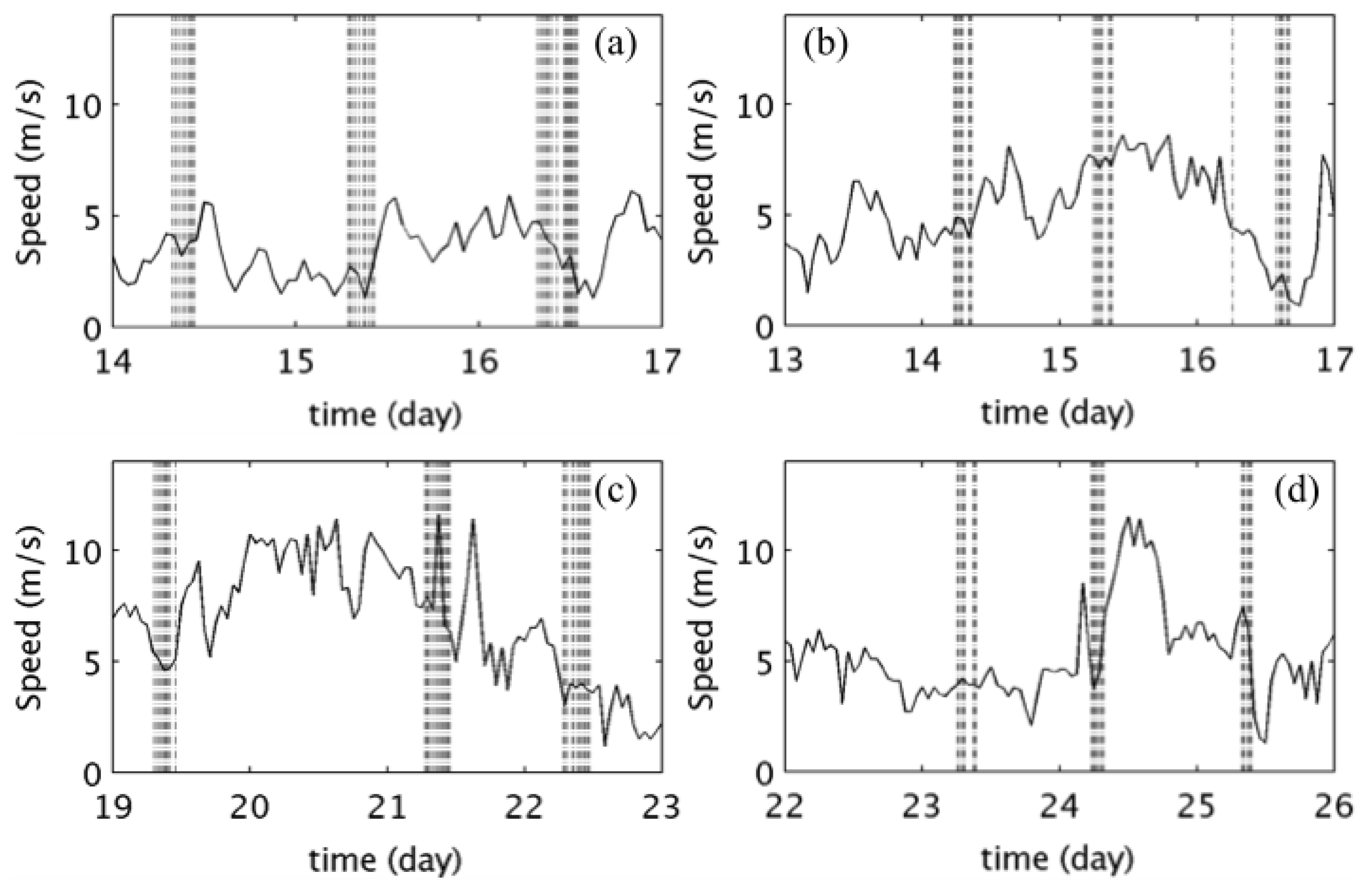
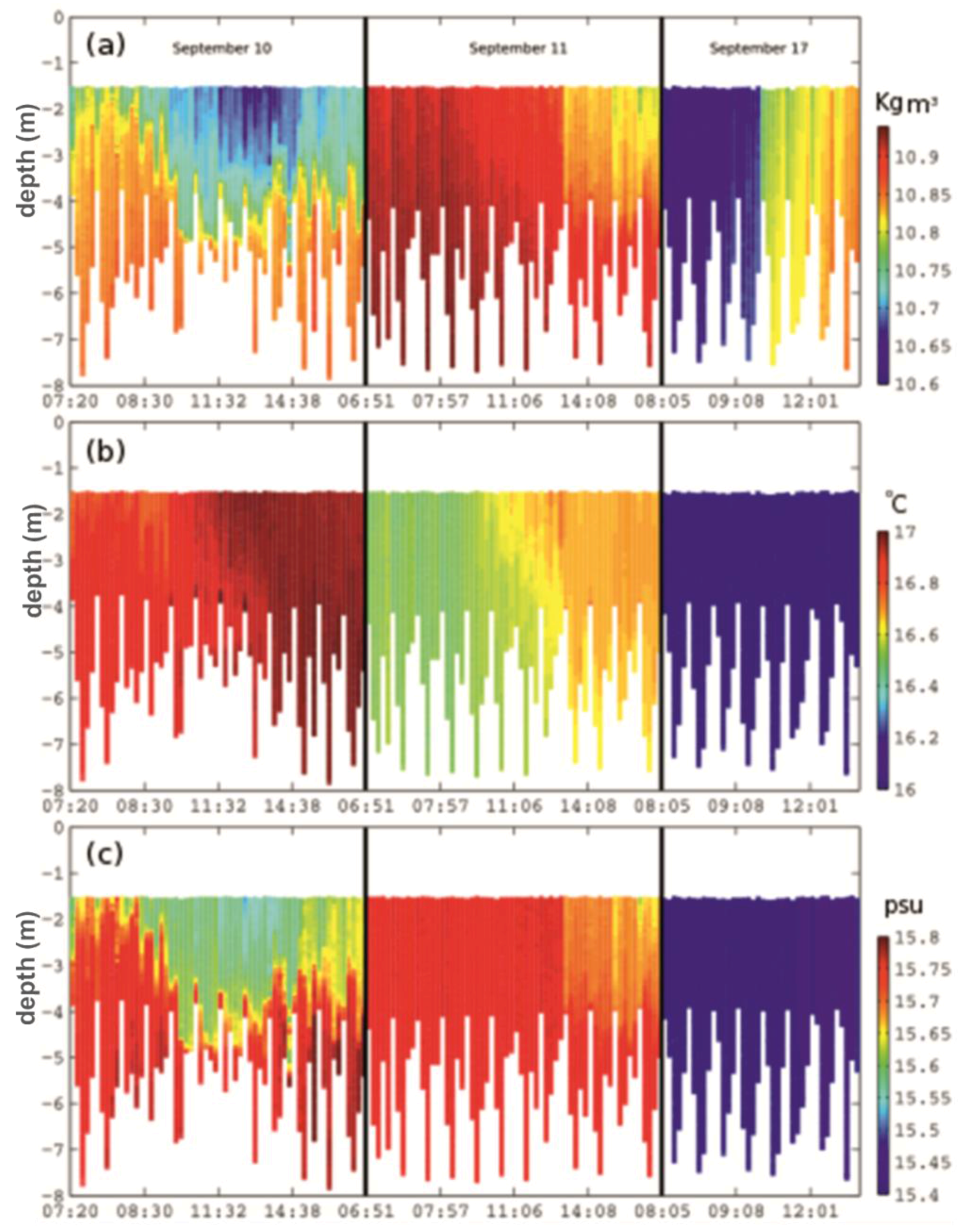
The hydrology of a deep (~4 m) excavation hole in the coastal inlet was investigated with a high-resolution sampling program to analyze mixing events and oxygen conditions in the water column. On 10, 11 and 17 September 2013, a total of 160 CTD casts were collected along a transect of 5 stations crossing one of the excavated holes and the surrounding area (Figure 1). Up to four parameters were included at each station: temperature, salinity, density and oxygen profiles as well as wind speed and direction data collected at the Assens’ weather station, in order to examine the effects of wind on the hydrodynamics around the pit.

3.5. Numerical Modeling of the Ocean Dynamics

Environmental monitoring was accomplished by means of high-resolution numerical models to simulate the mixing of the water layers and evaluate a possible range of environmental parameters which could bring about critical conditions.

Several different environmental models are available for this purpose. Wind wave modeling can describe the physical processes of wave generation, dissipation and wave-wave interaction [20,21,22,23]. These models have been validated by means of remote and in-situ observations [24,25,26,27] and have been used for different environmental applications [28,29,30,31]. Similarly, Ocean Circulation Models can describe the velocity field, physical parameters as temperature, salinity and turbulence which characterize the physical and biological processes affecting water quality. These high resolution, non-hydrostatic ocean models, have been often used to describe the turbulent mixing regimes of the water column [32].

The dynamics of the mixed layer in the Nørrefjord was investigated with a 1D general ocean turbulence model (GOTM, [33,34]). Using 60 vertical levels over a depth of 9 m, the model simulated 24 h employing a range of constant wind stress as atmospheric forcing and different stratification conditions for the water column. A time step of 30 s and a κ-ε turbulence closure model was used while mixed layer depth (MLD) was estimated using a threshold on turbulence kinetic energy of κ =10⁻⁵ m² s⁻². The wind speed values, W, ranged between 1 ms⁻¹ to 10 ms⁻¹ and the wind stress (τ), which is the horizontal force of the wind on the sea surface, was calculated as:

τ = C_d ρ_a W²

(1)

where C_d = 1.5 × 10⁻³ is the drag coefficient, and ρ_a = 1.2 kg m⁻³ is the density of air. In the model, the stratification of the water column was manipulated by assuming an average temperature profile in May and variable salinity profiles (S). The stratification index was then calculated from the square root of the Brunt–Väisälä frequency:

ϕ = √(g/ρ₀ ∂ρ/∂z)

(2)

where g is the gravity, ρ₀ is the average water density and z is the depth of the water column.

To evaluate horizontal and vertical transport across the sand pit, we applied a 3D non-hydrostatic model, the Bergen Ocean Model (BOM). BOM was developed by the University of Bergen and it solves the full three-dimensional primitive equation system [35,36]. The model calculates velocity field, pressure, density, salinity and temperature governed by momentum, mass conservation and the continuity equations. The discretization method uses an Arakawa-C staggered grid with σ-coordinate in the vertical. The model is applied to a square area of 30 m sides and includes a sand pit in the center. The model includes the effects of non-hydrostatic pressure and uses a domain of 60 × 60 horizontal points and 81 vertical layers. Hence, a 0.5 m resolution is used in the horizontal plane and between 5–10 cm in the vertical plane. We simulated 3D scenarios of 3 h length using a time step of 0.2 s and a range of constant wind stress over a realistic stratification structure. A non-reflective boundary condition at the open boundaries and zero velocities at the bottom boundary were applied. The model was executed using a Message Passing Interface language on a 16 cores cluster.

4. Results

4.1. Wind and Temperature Influence on Density Stratification

The surface circulation in the Nørrefjord is tightly linked to wind conditions, which are characterized by different speeds during the year (Figure 2). In particular the average wind speed from 13 to 17 May 2008 was 3.8 m s⁻¹ (Figure 2a), while from 18 to 23 August 2008 it was 6.5 m s⁻¹ (Figure 2c). In 2008, the different wind conditions were clearly reflected in the profiles of temperature and salinity observed with the repeated CTD casts (Figure 3a,b). In case of weak wind conditions (May 2008) a well-defined picnocline between 6 m and 8 m was driven by both changes in temperature and salinity (red and blue profiles), while in August 2008 well-mixed conditions were present due to stronger winds (Figure 3a). In May 2008, temperatures ranged between 15–16 °C at surface level, to 10 °C at the bottom, while it was much colder in May 2009 with a uniform distribution around 12 °C (Figure 3c). On the other hand, in August 2008 and 2009, the temperature was homogeneous along the water column and its value was around 18–20 °C. Similar patterns were observed for salinity profiles in 2008 and in 2009 (Figure 3). In May 2008, salinity value was 12 psu in the upper 5 m and increased steadily up to 18 psu at 10 m depth (Figure 3a). In August 2008, a value around 15 psu was present at all depths while a uniform value of 17 psu was observed in August 2009 (Figure 3c,d).

4.2. Hydrography across the Sand Pit

The excavated areas were characterized by high variability of the hydrographic conditions recorded from 9 to 18 September 2013 (Figure 4a). In particular, stratified conditions of the water column can build during the day but are quickly lost as soon as changes in wind conditions or changes in larger scale circulation occur, as shown below (Figure 4). The first day of sampling, lateral advection of fresh water (salinity values are around 15.4 psu) entered the area, driving changes in density profiles and stratification conditions (Figure 4b). These conditions persisted throughout the first day (~4:00 p.m.). During the second day of sampling, the relatively strong stratification condition was lost within a few hours because of overnight cooling (Figure 4c).

Indeed, temperature decreased from 17 °C to 16.5 °C and salinity increased to 15.75 psu. During the day (around 1:00 p.m.) a weak thermal stratification was seen to build up as well as a weak stratification in the density profiles (Figure 4c). This weakly stratified condition was present only at low wind regimes (~3 m/s, Figure 4a). Day 3 sampling was on 17 September, seven days after the last sampling. This was due to strong wind conditions (up to 14 m/s) prevailing from 14 September to 18 September in the area which prevented the sampling operations (Figure 5a). Thus, the hydrographic conditions observed in 17 September were quite different from the first two days, but showed patterns consistent with the effects of strong wind mixing and cooling of the water column (Figure 4).

4.3. Dynamics of Oxygen Saturation

Oxygen saturation is the relative measure between the dissolved oxygen concentration and the oxygen solubility in equilibrium. For surveying periods in 2008, the oxygen concentration was always very close to equilibrium, hence saturation was around 100% (Figure 3b). In particular, we noted that only positive values in the range from 101% to 102% were observed in 2008. Moreover, changes in salinity concentration were related to oxygen distribution (Figure 3b). Lower salinity was typically associated to lower oxygen saturation while higher surplus of oxygen was present in the deeper layers, possibly reflecting changes in the biological productivity. Data for 2009 showed a different situation: the water in May was mainly close to equilibrium (oxygen saturation around 100%), but at around T = 14 °C and S = 13.5 psu a body of unsaturated water was present (Figure 3d). In August 2009, the water column was mainly under-saturated with minimum values of oxygen saturation at about 65%. When sampling at high temporal frequency across the sand pit in 2013, patterns in oxygen distribution were visible both in the vertical and throughout the days (Figure 5b,c). However, the range of variability was small since oxygen concentration was always within 8.3–9.1 mg L⁻¹. The oxygen saturation (Figure 5b) showed a deficit (92%) or surplus (107%) during the first and the second day, respectively, whereas the well mixed conditions of the third day showed oxygen values close to equilibrium conditions (~100% oxygen saturation in Figure 5b).

Continuous oxygen measurements at the bottom of the sand pit were highly variable in time, in both 2008 and 2009 (Figure 6). Nonetheless, there was a provable seasonal pattern in the oxygen concentration at the bottom. Often the oxygen concentration reached a minimum at the end of the summer when the seawater temperature was high, stratification stronger, and there was an abundance of dead material sinking to the bottom. In fact, long periods (up to 30 days) of hypoxic conditions were observed during the summer of 2009 and with lower frequency in 2008. These low oxygen periods are however highly variable.

Significant changes in oxygen concentrations occurred in seasonal scales as well as within a few hours. In particular, in 2009 the oxygen concentration on 28 June was around 8 mg L⁻¹ and decreased to almost zero within three days (Figure 6). These changes were most likely driven by biological production as suggested for example by the large daily variation in oxygen, which is associated with negligible changes in temperature, salinity and hence solubility conditions. Nevertheless, on longer time scales, a correlation between wind speed and oxygen saturation was evident (Figure 6). This correlation was further explored using the entire dataset including 2008 and 2009 data (Figure 7), showing that an oxygen surplus could occur at low or high wind speed conditions, while oxygen deficit and anoxic conditions were more likely to occur at low wind speeds (2–4 m s⁻¹). Moreover, with high wind speeds (>12 m s⁻¹) only 100% oxygen saturation was present; over-saturated or under-saturated conditions were never recorded at high wind speed conditions (Figure 7). This supported the hypothesis of biology mediated effects on oxygen saturation conditions.

Thus, biological production can be inhibited by strong wind conditions, while in conditions of low wind speed and stratified water columns it can reach a maximum, favoring over-saturated conditions in the upper layers, or possibly hypoxia can develop in the deepest layers.

4.4. Numerical Simulation of the Mixed Layer Dynamics

To investigate the frequency of occurrence of these low oxygen levels at the bottom of a sand pit, we ran a set of numerical models to simulate the vertical mixing of a tracer induced by wind velocity. Simulations of 1D water column suggested that the balance between stratification and shear produced by the wind stress was responsible for the dynamics of the mixed layer depth (MLD) (Figure 8).

The depth of the mixed layer appeared to be mainly controlled by wind conditions: <4 m at wind speed values less than 3 m s⁻¹, within 4–6 m at wind speed values of 4–5 m s⁻¹ and 9 m (the total depth) at wind speed above 8 m s⁻¹. For intermediate wind speed values (5–7 m s⁻¹), a full mixed water column was simulated if the stratification was weak. In other words, with winds above 8 m s⁻¹ the entire water column was well mixed within 24 h, while between 6 and 8 m s⁻¹ the water column was either well mixed or stratified, largely depending on the density profile used in the model.

To establish the time scales and the range of wind velocity at which vertical mixing can reduce bottom oxygen depletion, a 3D model was used to simulate dispersion of a passive tracer under the non-hydrostatic circulation across a sand pit (Figure 9).

The tracer was initially released close to the bottom and the model simulated the effects of different wind conditions acting on a summer stratified water column initially at rest. Since the wind was blowing from the left to the right of this shallow depth section, we would expect a flushing of the bottom layers all across the domain in the direction of the transport. However, at wind speeds of 3–5 m s⁻¹, he pit was not significantly affected by wind mixing during the simulated 3 h; in fact, high concentrations of the tracer were still present in the pit at the end of the simulations. More likely, the shape of the pit was controlling the recirculation in the excavated pit than favoring water retention. Moreover, adjacent areas were also affected by the presence of the excavation. The up-wind side at 4 m depth had low tracer concentration while the down-wind kept a high tracer concentration due to the transport of tracer from the pit. This pattern was reversed at wind speed ≥7 m s⁻¹, due to turbulent vortices being created by the interaction between wind-driven current and the slope of the pit. With a stronger wind scenario (13 m s⁻¹), a complete mixing of the bottom layer was obtained by the end of the simulated period (Figure 9).

5. Discussion

Oxygen depletion at the bottom of a deep sand pit depends on a combination of physical and biological factors. A significant stratification of the water column hinders the downward oxygen transport by turbulence. This stratification is caused mainly by the increased water depth and reduced flow velocity, so that thermal stratification can occur in the spring and summer months. Both experimental evidence and numerical simulations showed a limited occurrence of conditions that can potentially lead to hypoxia. In fact, the number of consecutive days in which very low oxygen concentrations were recorded is lower than 10 (lowest level reported in the literature), while the numerical simulations show that the risk conditions are related to wind speeds lower than 5 m/s, which is infrequent in Danish waters. The inner Danish waters have experienced a gradual decrease in levels of oxygen in the bottom waters since the 1960s [37] due to increasing nutrient loadings, primarily from agricultural sources since the 1950s. The nutrient loading culminated in the late 1980s, at which time several mitigating measures were implemented to reduce nutrient loadings from several sources. Nørrefjord has also received considerable amounts of nutrients from the surrounding landscape during the last three to four decades causing habitat deterioration and decline in extent and distribution of blue mussel beds [38]. Oxygen depletion has also been reported to occur regularly in Nørrefjord, in the deep basin in late summer, although it has only been observed for a limited number of days. Nutrient loading persists, even though at lower levels than in the 1980s and may continue to cause periods of anoxia, which together with the conditions in the extraction pits and the restricted water exchange may slow down the process of recovery in this fjord.

There is a seasonal pattern in the oxygen concentration at Norrefjord. During winter, the oxygen concentration increases and reaches a maximum in May. Afterwards, the oxygen concentration reaches a minimum at the end of the summer when the seawater temperature is high and there is an abundance of dead material from algal blooms. In these conditions, there is a high risk of hypoxia at the bottom of the sand pit. The area impacted by sand mining shows clear patterns in terms of oxygen dynamics. The water column is fully saturated with oxygen in this area, when the winds are strong (>10 m s⁻¹), which is a relatively frequent situation especially outside the summer months. In particular, we find that the water column is completely mixed in the sand pit when wind is stronger than 8 m s⁻¹. According to the simulations using the 1D model, when wind speed is stronger than 8 m s⁻¹ for at least 24 h, active mixing is present at the depth of 9 m and the water column is fully mixed. On the other hand, oxygen depletion and oxygen surplus conditions (due to biological production) occur at wind speed lower than 5 m s⁻¹.

In particular, hypoxic layers frequently develop in summer, when strong water column stratification and a weak wind regime allows both the sinking of organic material and the dampening of the wind-driven mixing. Under these conditions strong oxygen-depletion and anoxic layers are developed within a few hours. When the oxygen-depleted zone is created then with a wind speed >8 m s⁻¹ the sand pit could act as a source of low oxygen for adjacent areas. This pattern is confirmed by the more detailed and computationally expensive 3D model, which shows that the regions located down-wind relative to the sand pit can be affected by transport of low oxygen concentrations from the sand pit. The 3D model also shows that the excavated area is effectively mixed over short time periods when winds are very strong (>13 m s⁻¹). However, these strong winds are quite rare in the area during summer months.

The study area is a coastal inlet characterized by very shallow water (<5 m). The shallow depth supports rapid changes of the environmental conditions in the water, such as temperature, salinity and oxygen concentration. These changes are mainly driven by wind patterns in terms of both direction and speed. The observed variability in oxygen concentration can be explained as a combination of the effects of temperature, salinity and wind speed, which influence the depth of the mixed layer but also biological productivity.

6. Conclusions

Waters with high residence times in areas of restricted exchange may experience considerable oxygen depletion in the presence of high amounts of oxygen consuming organic matter. In the highly eutrophicated estuarine systems of the inner Danish waters, the risk evaluation of hypoxic events was developed from the computation of oxygen dynamics as a function of the wind-driven mixing. The Danish measures implemented to reduce nutrient loadings have resulted in reduced inputs, but the accumulation of internal nutrient pools in the sediments and increased stratification may delay system recovery [39].

The persistent presence of extraction pits may further hinder the process towards system recovery in the Nørrefjord. In fact, the observed evidences and the obtained numerical results taking into account numerical simulations and extensive monitoring of the main physical parameters, cannot completely exclude intolerable oxygen conditions for the benthic communities in proximity of excavated sand pits. Hypoxic events have been observed during warm and calm summer months, because oxygen depletion may develop near the bottom in sand pits mainly at low wind speeds or, alternatively, when the wind is strong but blows for short periods. In autumn and winter strong winds and the general cooling and convective mixing of the water column exclude formations of oxygen depleted conditions.

The predictions of the vertical mixing inside the pit according to wind forcing, evaluated by a numerical model, established the range of parameters for which the occurrence of conditions favoring oxygen-depletion can develop inside the sand pit.

The elements identified in this study can be articulated in view of the recovery process to improve the status of degraded coastal and estuarine ecosystems. Existing studies indicate that complete recovery of coastal ecosystems to their previous baseline is rarely a realistic assumption [40]. The results obtained imply that pressures giving rise to eutrophication need to be reduced below the threshold levels, the crossing of which originally brought about the degradation, to obtain at least a partial recovery. In this context, the results of this study are a valuable input for future management of marine mineral aggregate extraction to guide the choice of extraction method, thus leading to a reduced environmental impact of such pits.

References

1. Meire, L.; Soetaert, K.; Meysman, F. Impact of global change on coastal oxygen dynamics and risk of hypoxia. Biogeosciences 2013, 10, 2633–2653. [Google Scholar] [CrossRef] [Green Version]
2. Rabalais, N.N.; Dıaz, R.J.; Levin, L.A.; Turner, R.E.; Gilbert, D.; Zhang, J. Dynamics and distribution of natural and human-caused hypoxia. Biosciences 2010, 7, 585–619. [Google Scholar] [CrossRef]
3. Diaz, R.J.; Rosenberg, R. Spreading dead zones and consequences for marine ecosystems. Science 2008, 321, 926–929. [Google Scholar] [CrossRef] [PubMed]
4. Sasaki, J.; Kawamoto, S.; Yoshimoto, Y.; Ishii, M.; Kakino, J. Evaluation of the amount of Hydrogen sulphide in a dredged trench of Tokyo bay. J. Coast. Res. 2009, I, 890–894. [Google Scholar]
5. Zhu, Z.; Isobe, M. Criteria for the occurrence of wind-driven coastal upwelling associated with “Aoshio” on the southeast shore of Tokyo Bay. J. Oceanogr. 2012, 68, 561. [Google Scholar] [CrossRef]
6. Zhu, Z.; Bai, X.; Dou, J.; Hei, P. Applying a Simple Analytical Solution to Modelling Wind-Driven Coastal Upwelling of Two-Layered Fluid at the Head of Tokyo Bay, Japan. Water 2017, 9, 744. [Google Scholar] [CrossRef]
7. Pearson, T.H.; Josefson, A.B.; Rosenberg, R. Petersen’s benthic stations revisited I Is the Kattcgatt becoming eutrophic? J. Exp. Mar. Biol. Ecol. 1985, 92, 157–206. [Google Scholar] [CrossRef]
8. Rosenberg, R.; Loo, L.O. Marine eutrophication induced oxygen deficiency effects on soft bottom fauna, Western Sweden. Ophelia 1988, 29, 213–225. [Google Scholar] [CrossRef]
9. Breitburg, D. Effects of hypoxia, and the balance between hypoxia and enrichment, on coastal fishes and fisheries. Estuaries 2002, 25, 767. [Google Scholar] [CrossRef]
10. Behrens, J.W.; Ærtebjerg, G.; Petersen, J.K.; Carstensen, J. Oxygen deficiency impacts on burying habitats for lesser sandeel, Ammodytes tobianus, in the inner Danish waters. Can. J. Fish. Aquat. Sci. 2009, 66, 883–895. [Google Scholar] [CrossRef]
11. Conley, D.J.; Björck, S.; Bonsdorff, E.; Carstensen, J.; Destouni, G.; Gustafsson, B.G.; Hietanen, S.; Kortekaas, M.; Kuosa, H.; Meier, H.E.M.; et al. Hypoxia-related processes in the Baltic Sea. Environ. Sci. Technol. 2009, 43, 3412–3420. [Google Scholar] [CrossRef] [PubMed]
12. Hoogewoning, S.E.; Boers, M. Fysische Effecten van Zeezandwinning (Physical Effects of Sea Sand Extraction); RIKZ/2001.050; Rijksinstituut voor Kust en Zee/RIKZ: The Hague, The Netherlands, 2001; p. 95. (In Dutch) [Google Scholar]
13. De Groot, S.J. Marine sand and gravel extraction in the North Atlantic and its potential environmental impact, with emphasis on the North Sea. Ocean Manag. 1986, 21–36. [Google Scholar] [CrossRef]
14. Mudge, S.; Icelyb, J.D.; Newtonc, A. Oxygen depletion in relation to water residence times. J. Environ. Monit. 2007, 9, 1194–1198. [Google Scholar] [CrossRef] [PubMed]
15. Boers, M. Effects of a Deep Sand Extraction Pit; Final Report of the PUTMOR Measurements at the Lowered Dump Site. Rapport RIKZ/2005.001; RIKZ: The Hague, The Netherlands, 2005. [Google Scholar]
16. De Groot, S.J. The physical impact of marine aggregate extraction in the North Sea. ICES J. Mar. Sci. 1996, 53, 1051–1053. [Google Scholar] [CrossRef]
17. Krause, J.W.; Brzezinski, M.A.; Landry, M.R.; Baines, S.B.; Nelson, D.M.; Selph, K.E.; Taylor, A.G.; Twiningf, B.F. The effects of biogenic silica detritus, zooplankton grazing, and diatom size structure on silicon cycling in the euphotic zone of the eastern equatorial Pacific. Limnol. Oceanogr. 2010, 55, 2608–2622. [Google Scholar] [CrossRef]
18. Saviour, M.N. Environmental impact of soil and sand mining: A review. Int. J. Sci. Environ. Technol. 2012, 1, 125–134. [Google Scholar]
19. Poulsen, L.K.; Christensen, H.T.; Stenberg, C.; Kristensen, L.D.; Thorsen, S.W.; Røjbek, M.; Landes, A.; Andersen, S.K.; Dolmer, P.; Geitner, K. Slutrapport for Projekt BioRev 2010; DTU Aqua Rapport nr. 251-2012; Institut for Akvatiske Ressourcer, Danmarks Tekniske Universitet: Lyngby, Denmark, 2012; p. 51. ISBN 978-87-7481-152-7. [Google Scholar]
20. WAMDI Group: TheWAM model—A third generation ocean wave prediction model. J. Phys. Oceanogr. 1988, 18, 1775–1810.
21. Tolman, H.L. Effects of numerics on the physics in a third-generation wind-wave model. J. Phys. Oceanogr. 1992, 22, 1095–1111. [Google Scholar] [CrossRef]
22. Benassai, G.; Ascione, I. Implementation of WWIII wave model for the study of risk inundation on the coastlines of Campania, Italy. WIT Trans. Ecol. Environ. 2006, 249–259. [Google Scholar] [CrossRef]
23. Benassai, G.; Ascione, I. Implementation and validation of Wave Watch III model offshore the coastlines of Southern Italy. In Proceedings of the 25th International Conference on Offshore Mechanics and Arctic Engineering, Hamburg, Germany, 4–9 June 2006. [Google Scholar] [CrossRef]
24. Montuori, A.; Ricchi, A.; Benassai, G.; Migliaccio, M. Sea wave numerical simulation and verification in Tyrrhenian costal area with X-band cosmo-skymed SAR data. In Proceedings of the ESA, SOLAS & EGU Joint Conference Earth Observation for Ocean-Atmosphere Interactions Science, Frascati, Italy, 29 November–2 December 2012. [Google Scholar]
25. Benassai, G.; Migliaccio, M.; Montuori, A. Sea wave numerical simulations with COSMO-SkyMed© SAR data. J. Coast. Res. 2013, 660–665. [Google Scholar] [CrossRef]
26. Benassai, G.; Montuori, A.; Migliaccio, M.; Nunziata, F. Sea wave modeling with X-band COSMO-SkyMed© SAR-derived wind field forcing and applications in coastal vulnerability assessment. Ocean Sci. 2013, 9, 325–341. [Google Scholar] [CrossRef]
27. Benassai, G.; Migliaccio, M.; Nunziata, F. The use of COSMO-SkyMed© SAR data for coastal management. J. Mar. Sci. Technol. 2015, 20, 542–550. [Google Scholar] [CrossRef]
28. Benassai, G.; Stenberg, C.; Christoffersen, M.; Mariani, P. A sustainability index for offshore wind farms and open water aquaculture. WIT Trans. Ecol. Environ. 2011, 149, 3–14. [Google Scholar] [CrossRef]
29. Benassai, G.; Mariani, P.; Stenberg, C.; Christoffersen, M. A Sustainability Index of potential co-location of offshore wind farms and open water aquaculture. Ocean Coast. Manag. 2014, 95, 213–218. [Google Scholar] [CrossRef]
30. Benassai, G.; Di Luccio, D.; Migliaccio, M.; Corcione, V.; Budillon, G.; Montella, R. High resolution remote sensing data for environmental modelling: Some case studies. In Proceedings of the 2017 IEEE 3rd International Forum on Research and Technologies for Society and Industry (RTSI), Modena, Italy, 11–13 September 2017. [Google Scholar] [CrossRef]
31. Di Tullio, G.R.; Mariani, P.; Benassai, G.; Di Luccio, D.; Grieco, L. Sustainable use of marine resources through offshore wind and mussel farm co-location. Ecol. Model. 2018, 367, 34–41. [Google Scholar] [CrossRef]
32. Giunta, G.; Mariani, P.; Montella, R.; Riccio, A. pPOM: A nested, scalable, parallel and Fortran 90 implementation of the Princeton Ocean Model. Environ. Model. Softw. 2007, 22, 117–122. [Google Scholar] [CrossRef]
33. Stigebrandt, A.; Gustafsson, B.G. Response of the Baltic Sea to climate change—Theory and observations. J. Sea Res. 2003, 49, 243–256. [Google Scholar] [CrossRef]
34. Burchard, H.; Petersen, O. Models of turbulence in the marine environment—A comparative study on two-equation turbulence models. J. Mar. Syst. 1999, 21, 29–53. [Google Scholar] [CrossRef]
35. Burchard, H.; Bolding, K.; Kühn, W.; Meister, A.; Neumann, T.; Umlauf, L. Description of a flexible and extendable physical-biogeochemical model system for the water column. J. Mar. Syst. 2006, 61, 180–211. [Google Scholar] [CrossRef]
36. Berntsen, J. USERS GUIDE for a Mode Split Sigma-Coordinate Ocean Model. Version 1.0; Report No. 135; Department of applied mathematics, University of Bergen: Bergen, Norway, 2000. [Google Scholar]
37. Jørgensen, B. Seasonal oxygen depletion in the bottom water of a Danish fjord and its effects on the benthic community. Oikos 1980, 34, 68–76. [Google Scholar] [CrossRef]
38. Rask, N.; Bundgaard Madsen, H.; Larsen, S. Vandmiljøovervågning. Kystvande 1999; Fyns Amt: Odense, Denmark, 2000. [Google Scholar]
39. Riemann, B.; Carstensen, J.; Karsten, D.; Fossing, H.; Hansen, J.W.; Jakobsen, H.H.; Josefson, A.B.; Krause-Jensen, D.; Markager, S.; Stæhr, P.A.; et al. Recovery of Danish Coastal Ecosystems after Reductions in Nutrient Loading: A Holistic Ecosystem Approach. Estuaries Coasts 2015. [Google Scholar] [CrossRef]
40. Duarte, C.; Borja, A.; Carstensen, J.; Elliott, M.; Krause Jensen, D.; Marbà, N. Paradigms in the recovery of estuarine and coastal ecosystems. Estuaries Coasts 2015. [Google Scholar] [CrossRef]
Figure 1. Map of the Nørrefjord area on the southern side of the Funen Island in Denmark. The area impacted by sand mining (blue area) and the transect (red line) used in the high-resolution data acquisition are also shown.
Sustainability 10 00785 g001
Figure 2. Time series of the wind speed in: (a,c) 2008; and (b,d) 2009, in May (a,b) and August (c,d). Days of the CTD casts are reported in dashed lines. Corresponding profiles of temperature and salinity from the CTD casts in May and August are in Figure 3a,c (2008 and 2009, respectively).
Sustainability 10 00785 g002
Figure 3. Temperature and salinity in the CTD casts in Nørrefjord during the surveys in: (a,b) 2008; and (c,d) 2009. Profiles of temperature and salinity collected in May and August in: (a) 2008; and (c) 2009. Scatter plots of temperature against salinity with colors representing oxygen saturation (%) in: (b) 2008; and (d) 2009. The size of the points is log-distributed according to depth and larger dots are for deeper observations.
Sustainability 10 00785 g003
Figure 4. Distribution of: (a) density (kg m−3–1000); (b) temperature (°C); and (c) salinity (psu) in the 160 CTD casts on 10, 11 and 17 September 2013 across a transect crossing the sand pit.
Sustainability 10 00785 g004
Figure 5. Time series of the wind speed in the study area from 9 to 18 September. The three periods (grey areas) when CTD casts area available are also shown (a). Oxygen saturation against water density (b) for the three sampling periods: 10 September (red), 11 September (green) and 17 September (yellow); and corresponding oxygen distribution (mg L−1) in the 160 CTD casts on 10, 11 and 17 September across the study transect (c).
Sustainability 10 00785 g005
Figure 6. Time series of oxygen concentration (green) and wind speed (blue) in: (a) 2008; and (b) 2009. Oxygen levels were recorded at the bottom of an excavated hole.
Sustainability 10 00785 g006
Figure 7. Scatter plot (white symbols) of wind speed against oxygen saturation level. Data for 2008 and 2009 are averaged over 12 h.
Sustainability 10 00785 g007
Figure 8. Map of the simulated mixed layer depth (MLD) at different wind speeds and with a set of realistic density profiles based on observations made in May. The model runs for 24 h with constant wind, MLD for the last time step is shown and is calculated using a turbulent kinetic threshold of 10−5 m2 s−2. Stratification index is defined based on the density profiles, higher index in more stratified conditions.
Sustainability 10 00785 g008
Figure 9. Map of the tracer concentration on a vertical section across the sand pit. Values are shown at different time (columns): after 1, 2 and 3 h simulations with constant wind. Each row represents a different wind speed: 3 m/s (row 1); 5 m/s (row 2); 7 m/s (row 3); 13 m/s (row 4). Values are shown on a linear color range from 0 (blue) to 1 (red).
Sustainability 10 00785 g009