1. Introduction
Sustainability has been an important issue for several decades because companies want to secure competitive advantages for their future such as cost savings, consumer demand, risk mitigation, tax incentives, and using resources efficiently in saturated or competitive markets. The business environment has been changed by the enforcement of the global environment, an increase in green consumers, and economic loss due to lack of environmental control. Besides, firms’ economic burden has been increased by environmental regulations such as the reduction of emissions and greenhouse gas. We trace back to why it became an important agenda. At the G-8 summit meeting, 2007, the main agenda was sustainability due to global warming caused by climate change. The issues of energy and environment have been cardinal factors determining a nation’s economic future. According to the EPA (Environmental Protection Agency, Washington, DC, USA), a 2016 report states that three major factors provoke climate changes regarding earth’s energy balance, including (1) variations in the sun’s energy reaching earth; (2) changes in the reflectivity of earth’s atmosphere and surface; (3) changes in the greenhouse effect, which affects the amount of heat, and retaining earth’s atmosphere. Basically, in order to protect the environment, a lot of money is needed. The UNEP FI [
1] report says that the environmental costs generated by the top 3000 companies, which are responsible for 35% of total global externalities caused by human and economic activity, totaled
$2.15 trillion, including impacts from the operation and production of purchased goods and services. Even though the firms pay the environment costs, they not only should continue to pay for it because the government does not give them more incentives and beneficial policies but should also be in charge of corporate social responsibility. If they do not protect the environmental issues from which climate change, water scarcity, food security and deforestation have emerged, they are not able to obtain sustainable competitive advantages such as envisioning various scenarios for the future. Corporate sustainability is becoming significant as the mainstream for the current and future growth engine. In theoretical and empirical research papers, it was demonstrated why companies need a sustainable strategy because there was a positive relationship between sustainable management and financial returns as evidenced by [
2,
3,
4,
5,
6].
All activities regarding sustainability include more than the economic status. However, in general, sustainability cannot only have an influence on the economic growth, but is also germane to economic development. In other words, the major goal of economic growth is sustainability. When we categorize developed countries, the main criterion would be the economic growth and environmental constraints and risks. According to the global environmental outlook [
7], the Regional Environment Information Network (REIN) decided that the Asia-Pacific region is a priority to perform environmental actions with critical issues; in addition, it has the worst record of affecting 4.5 billion people, which caused a loss of
$1076 billion between 1990 and 2014. On the other hand, the environmental conditions in North America have significantly improved for a decade, considering investments in policies, institutions, data collection and assessment and regulatory frameworks.
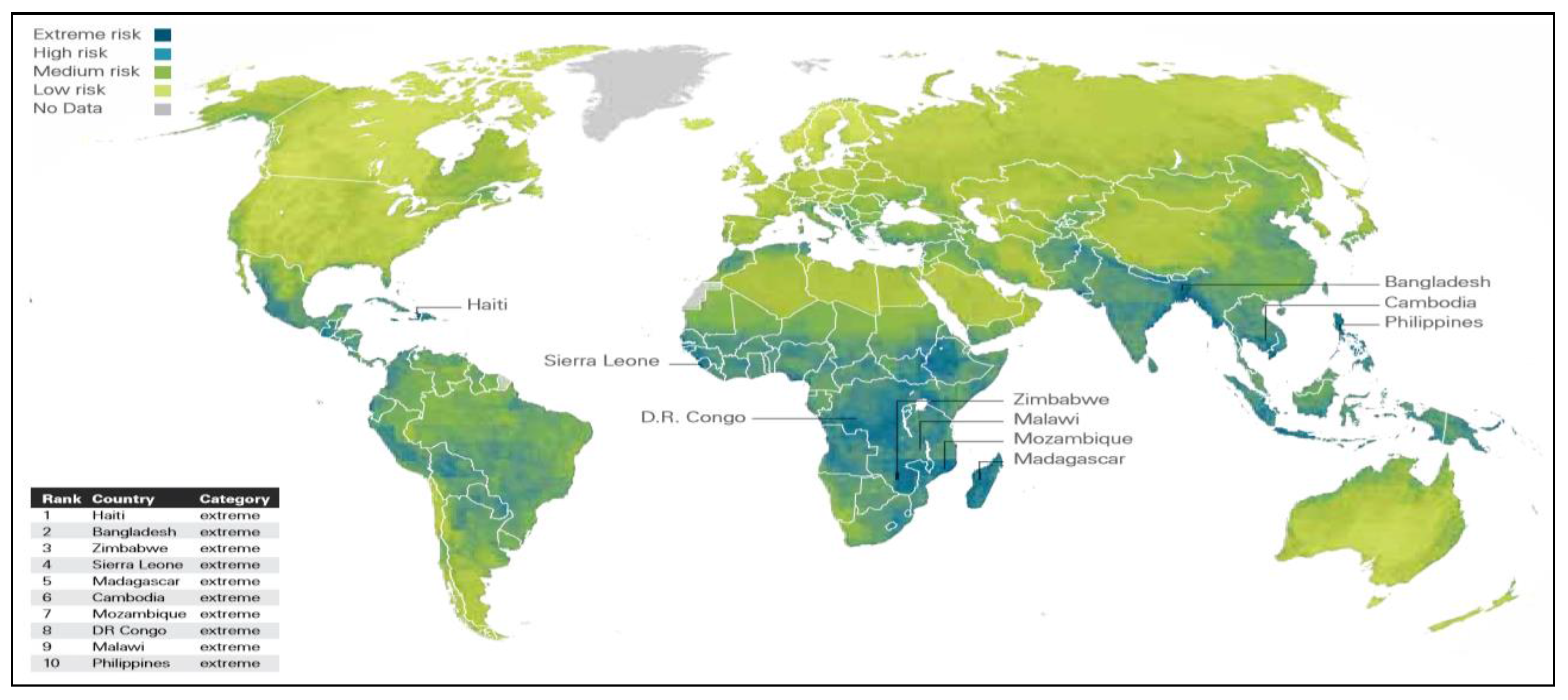
Figure 1 shows the vulnerability of climate change and environmental risk throughout the world. There are the global mega forces that affect water scarcity, energy and fuel, deforestation and ecosystem decline directly. This research focuses on North America and the Asia-Pacific region. As mentioned above, the environmental situation differs between the two regions. By comparing them, we corroborate that sustainable investment in well-performing regions leads to social and economic growth and environmental stability.
Based on a previous literature review, current research on the economics of sustainability is mainly historical [
8]. Besides, estimating sustainability is like a conundrum because it has two properties. Firstly, sustainability has a long-term value [
2]. Measuring the performance of sustainable activities requires precise data because it is not the only part of performance but is the result of the enterprise’s performance from each business unit, including the strategies and forecasting multiple scenarios over a long-term period. However, long-term values can be estimated accurately. This research uses on a long-term period between 10 and 20 years. In the stock market, similarly, there is a calculation method for sustainable growth rates using accounting rates such as in financial statements. Through predictive modeling, we attempt to prove corporate and economic performance relative to sustainable investment and management.
The purpose of this article is to substantiate that a firm’s sustainable activity is associated with financial performance, and the relationship between sustainable investment and economic development is the causality. We contribute to the sustainability literature, especially with respect to measuring sustainable investment and why companies should ensure sustainable management. We structure the article as follows. First, we provide the theoretical background from previous research on the corporate performance, investment, and economic development of sustainability. We apply this theoretical background to the sustainable investment index. We propose an empirical hypothesis linking affordable methodology such as VAR (Vector Autoregressive) and VECM (Vector Error Correction Model) in a time series model. We conclude with implications for research and practice and limitations.
3. Methods
VAR Properties. Our goal is to figure out causality among sustainability performance, financial returns, and economic development. To do this, we use the VAR (Vector Autoregressive) model. In former studies, they have been utilized by analyses such as financial data, stock prices/returns, and money supply by [
50,
51,
52]. The VAR model in economics was made popular by Sims [
53]. Especially, it is proven when describing the dynamic behaviors of economics and financial time series and for forecasting, and it has been known as the model from univariate autoregressive to multivariate autoregressive frequently used for projection and efficiency analysis by the change of endogenous variables. Zivot and Wang [
54] indicated that the VAR model is used for structural inference and policy analysis. In structural analysis, certain assumptions about the causal data structure are imposed and the resulting causal impacts of unexpected shocks or innovations are summarized. Utilizing the VAR model can show how an endogenous variable changes the dynamic response; our goal concentrates on the causality, not a correlation between investing sustainability and financial returns.
There is a difference between time-series and cross-sectional data. Based on the stationarity of a variable, time series analysis satisfies phenomenon’s assumption and is efficient. When variables of time series have non-stationarity, they have to be eradicated because the data should be detrended before estimating a specific VAR model. The first thing we do is to employ the Augmented Dickey-Fuller (ADF) and Phillips-Person (PP) unit root tests for the multivariate approach of Johansen and Juselius [
55]. After the ADF test, if the variable is non-stationary, we have to treat the first difference of the variable indicating that the non-stationary variable is modified into being stationary. Then, given the nature of the results, we can make a decision selecting the lag length. As denoted in
Table 2, our paper is embraced in ‘multivariate’ mode, analyzing our hypotheses by VAR and VECM. Why we chose this VAR model is that first, the impulse response analysis attests a change of one variable in endogenous variables influencing dynamic effects. Secondly, through the variance decomposition, we can analyze the size of the contribution of these variables to the total variation in each endogenous variation. What it means is that VAR does not settle the theoretical hypothesis by economic theory but analyzes real economic situations using given economic time series. In other words, it makes systematic outputs utilizing parallax variables like an explanatory variable relative to all variables.
Modeling and Data. In order to clarify the relationship between sustainability performance, financial returns, and economic development, we have garnered the variables such as the data of stock market regionally, each firm’s stock price, and macro economic factors. Many types of studies have demonstrated the relation among stock market, stock returns, and specific economic variables, i.e., [
56,
57,
58,
59,
60,
61]. This paper has different contributions in comparison with them. First, it extends regional stock markets in Asia-Pacific and North America, including a particular topic, sustainability performance empirically. The only conceptual ‘buildup’ was performed considerably because it is demanding to gather real data, and hardship exists in measuring quantitatively. Hence, we settle on a variable of sustainability by DJSI (Dow Jones Sustainability Index) because DJSI is an assessment model of sustainability considering financial, social, and environmental information.
In comparison with previous works, which are based on empirical methodology, our work differentiates macro and micro perspectives by using representative stock indices in Asia and North America and stock prices of individual firms. How we proceed ‘step by step’ for Hypothesis 1 is through two approaches; (1) selecting capital flows of major stock markets such as Nikkei 225, Shanghai-Shenzhen, KOSPI, AUS 200, and Hong Kong Hansen of Asia-Pacific and NASDAQ, S&P 500 of North America. These are all responsible for handling and organizing the investment in each region; (2) constituting stock prices of the top 5 sustainability companies of DJSI regionally; (3) using the variables of accounting of rates such as ROI, ROIC, and ROA from an investment company, ‘Five Tree’ in South Korea. Hypothesis 2 portrays the causality between sustainability performance and economic development by GDP per capita and GNI per capita. To prevent multicollinearity, it requires other variables because depending on the population, the values of GDP and GNI can show a discrepancy in which two predictors in multiple regression models are highly correlated, indicating that one variable may be linearly predicted from the others with an equivalent degree of accuracy. We focus on GNI and GDP as mentioned in theory building of the last section, albeit the macro economy has many indicators like money supply, CPI, and un/employment. The time setting for Hypothesis 2 is from 1998 to 2016 because economic development is not ‘fleeting innovation,’ while Hypothesis 1, which is germane to sustainability, settles on 2010 through 2016. Plus, all variables were modified to logarithms to set up the normal distribution in which the regression equation is stable.
When the time series variables have stationarity, the first model of the time series we can consider is the ARIMA. However, that has a limited option, utilizing only the information related to their past. In order to generally observe the relationship between each variable, the ARIMA model has some limitations that do not consider additional information such as factors. Therefore, we need to add the other variables influencing the dependent variable. By adding vectors, the AR model includes the scalar variable, while the VAR model deals with a vector, which means dependent and explanatory variables. Hypothesis 1 construes the causality between sustainability performance and economic value, especially financial returns. To do so, we use the VAR basic model in (1) as below:
where,
constitutes the vector, some “k” endogenous variable of analysis target. If we use the VAR model, it is possible to consider how other variables affect our objective variable,
. All time series variables should accord with stationarity so they prevent divergence of the significance of endogenous variables. If our variables have unsated stationary time series, we move to VECM (Vector Error Correction Model), in (1) following that to estimate the co-integration relationship, the stationarity satisfies added lagged variables,
Zt-1.
It is possible that VAR analysis can be applied to dummy variables [
46]. We define the dummy variables as zero and one (0, 1). When the GNI and GDP have a higher value compared to an average value in each time, the value is one, 1; Otherwise, zero, 0. As mentioned in
Table 3, we set another dummy variable such as GR (Great Recession) from 2008 to 2009 as these variables need to undergo shock mitigation, not influencing the other variables.
Preliminary Analysis: ADF and KPSS Test. In order to verify the stationarity of the VAR model, we employ the ADF and KPSS analysis of the unit root test individually. The estimation of the ADF test is in (3), and the null hypothesis is H
0:
= 0. We assume that if a null hypothesis cannot be rejected, the unit root exists.
Showing the consequences of ADF and KPSS test in
Table 4, we reject the null hypothesis, meaning that unit root exists. However, after the first difference in the KPSS test, all variables have stationarity. In this regard, Eagle and Granger [
62] substantiated that even if there is a change of trend in individual economic time series to an abnormal set (or unstable) and if the linear combination having stationary time series over the long-term exists, the linear combination becomes a stationary time series variable. In other words, these time series variables are in a co-integrating relationship. However, co-integrated method of Eagle and Granger [
62] has the deficiency when the co-integrating vector has a value of two or more. Johansen [
63] found that when variables are non-stationary, it is possible to modify the alternatives using the vector error correction model (VECM) after performing the co-integration test. As we settle on not only a standard of time series analysis in
Table 2, but also a literature review as mentioned above, the remainder of the variables are operated on by the vector error correction model (VECM) except for log(ND), log(NTD), and log(AP GDP). To lay the groundwork for VECM, we first perform the co-integration test such as the Johansen test (See Appendix A.1 in Supplementary Materials).
After ADF and the KPSS test, we know how variables should be organized in the VAR or VECM. The time series analysis does not mean a theoretical prediction model but an extended prediction model when a real situation happens in social issues or business sectors. As mentioned above, we structure the VAR and VECM respectively by inserting our variables as in the examples of Equations (3) and (4) below. An equation does not indicate the matrix of each variable.
4. Results
Table 5 shows the summary statistics. According to the result of Hypothesis 1a, using VECM in daily data from 2010 to 2015, sustainability performance in the Asia-Pacific region is positively associated with Asia major stock markets such as AUS (<0.00001), SS (0.07), KP (0.007) in
Table 6. The rest, NK, and HKH, however, are not significant with sustainability total returns. As determinants of variable stationarity, eigenvectors are 0.05, 0.03, 0.02, 0.01, 0.008, and 0.005, indicating that they are stationary, i.e., less than one, ‘1’ (See the Appendix A.1.1 in Supplementary Materials). In North America, the consequences of VECM show that ND and SP have a strong relationship with sustainability performance. Albeit many companies are registered in ND and SP, which are pertinent to the investment and financial returns like economic values. That is a crucial reason why this research determines vector autoregressive analysis instead of correlation between the variables. Their eigenvectors between Asia Pacific and top 5 companies in the Asia Pacific area are stationary. In other words, this VECM is stable (See Appendixes A.1.2 and A.1.3 in Supplementary Materials).
Table 7 indicates that sustainability has the positive relationship between the DJSI of North America and stock market’s flow like NASDOQ.
In order to verify the relation between sustainability performance and financial returns, we estimate the causality with specific variables for Hypothesis 1b.
Table 8 and
Table 9 show that most of top 5 companies, which are sustainable in each region, are germane to financial returns. Of course, statistically, several companies such as SE, TM, SH, and WB in The Asia-Pacific region, also AI, JJ, and VZ in North America, are not significant but as seen in
Table 10, AP, TM, SH, and WB are all significant with sustainability total returns after individual VECM analysis by exposing them to endogenous variables. That is because, in one of the properties in VAR, it is not necessary to worry which variable is the endogenous variable and which is the exogenous variable [
64]. The remainders of independent variables, AI, JJ, and VZ are not significant with respect to sustainability total returns even after analyzing individual VECM. Here, there is an implication that we need to categorize by industry and then to figure out why these companies have significance through an in-depth case study.
Causalities among the variables are shown in
Table 11. Hypothesis 1c is substantiated. In North America and The Asia-Pacific region, the financial earns of investment are germane to sustainable management in their firms. All
p-values in ROI, ROIC, and ROA are significant. Besides, adjusted
R-squared values indicating explanatory power between variables are high in The Asia-Pacific region especially. As mentioned for ROI and ROIC, these results indicate that there are causalities between the efficiency of investment and sustainable management. It assumes carefully that high sustainable management will be outperformed in comparison with not ensuring sustainable management. We accentuate that sustainable management encompasses all of the corporate processes. To preserve the environment, the firms have to not only develop technologies using their core competencies but also to distribute the contribution to society; they try to solve the poverty as volunteers, donating one part of their revenues. Plus, by assuming organizational governance, the firms let investors know that a company uses accurate and transparent accounting methodologies.
As considerable literature has suggested for the relation between macroeconomic variables and economic growth, our paper has the characteristics of analyzing real and authentic data of sustainability, a firm’s accounting of rates, and macro-economic variables like GDP per capita and GNI per capita. As a result,
Table 12 shows that the relationship between an economic development and sustainability index in the Asia Pacific is manifested as the GDP(0.05915) and GNI (0.03319) being significant, and sustainability total returns in The Asia-Pacific region and eigenvalues are stationary, less than ‘1’ (See Appendixes A.1.1 and A.1.2 in Supplementary Materials). North America’s consequences of GDP and GNI relative to sustainability are 0.00088 and 0.0285, respectively.
As to Hypothesis 2a, the relation between GNI in North America and sustainability investment is positively pertinent (Refer to
Table 13). To test Hypothesis 2b, we use forecast error variance decomposition. The difference between regions exists precisely. In the Asia-Pacific region, for example, after the 15th quarters, sustainability variance explains 65.59%. Meanwhile, GDP and the population of variance contribute to sustainability with 9.86% and 24.55%(Refer to
Table 14), respectively, while in North America, sustainability variance is 51.03%, and the rest of the variances account for GDP 24.68% and population 2.56%. Depending on the quarters, we know how the values of indicators like sustainability and GDP can be predicted. The findings for Hypothesis 2b then provide not vague explanations but support for an idea of why sustainability in The Asia-Pacific region has importance for the future because it would be the overarching factor for the near future. In summary, the results are consistent with the hypotheses developed above. We know the ramification of how sustainability impacts financial returns and how economic development influences several industries (See Appendix C in Supplementary Materials).


