Abstract
We introduce and analyze a simple formal thought experiment designed to reflect a qualitative decision dilemma humanity might currently face in view of anthropogenic climate change. In this exercise, each generation can choose between two options, either setting humanity on a pathway to certain high wellbeing after one generation of suffering, or leaving the next generation in the same state as the current one with the same options, but facing a continuous risk of permanent collapse. We analyze this abstract setup regarding the question of what the right choice would be both in a rationality-based framework including optimal control, welfare economics, and game theory, and by means of other approaches based on the notions of responsibility, safe operating spaces, and sustainability paradigms. Across these different approaches, we confirm the intuition that a focus on the long-term future makes the first option more attractive while a focus on equality across generations favors the second. Despite this, we generally find a large diversity and disagreement of assessments both between and within these different approaches, suggesting a strong dependence on the choice of the normative framework used. This implies that policy measures selected to achieve targets such as the United Nations Sustainable Development Goals can depend strongly on the normative framework applied and specific care needs to be taken with regard to the choice of such frameworks.
1. Introduction
The growing debate about concepts such as the Anthropocene [1], Planetary Boundaries [2,3,4], and Safe and Just Operating Spaces for Humanity [5], and the evidence about climate change and approaching tipping elements [6,7] shows that humanity and, in particular, the current generation has the power to shape the planet in ways that influence the living conditions for many generations to come. Many renowned scholars think that climate change mitigation by a rapid decarbonization of the global social metabolism is the only way to avoid large-scale suffering for many generations, and some suggest a “carbon law” by which global greenhouse gas emissions must be halved every decade from now [8] to achieve United Nations Sustainable Development Goals within planetary boundaries. Others argue that such a profound transformation of our economy would lead to unacceptable suffering at least in some world regions as well, at least temporarily, and suggest that instead of focusing on mitigation, the focus should be on economic development so that continued economic growth will enable future generations to adapt to climate change. Still others advocate trying to avert some negative impacts of climate change by large-scale technological interventions aiming at “climate engineering” [9,10]. Since a later voluntary or involuntary phase-out of many climate engineering measures can have even more disruptive effects than natural tipping elements [11], one should, of course, also be concerned that a focus on climate engineering and, maybe to a somewhat lower degree, also a focus on adaptation might increase humanity’s dependence on large-scale infrastructure and fragile technology to much higher levels than we learned to deal with, posing a growing risk of not being able to manage these systems forever.
While one might argue that there does not need to be a strict choice between either mitigation or adaptation, the presence of tipping elements in both the natural Earth system and in social systems [12], and the likelihood of nonlinear feedback loops between them [13], suggests that only significant mitigation efforts will avoid natural tipping, and only significant socio-economic measures will cause the “social” tipping into a decarbonized world economy that is no longer fundamentally based on the combustion of fossil fuels. This means the current generation may face a mainly qualitative rather than a quantitative choice: do or do not initiate a rapid decarbonization? Additionally, this choice might take the form of a dilemma where we can either pursue our development and adaptation pathway and put many generations to come at a persistent risk of technological or management failure, or get on a transformation pathway that sacrifices part of the welfare of one or a few generations to enable all later generations to prosper at much lower levels of risk.
While all this might seem exaggerated, we believe that as long as there is a non-negligible possibility that, indeed, we face such a dilemma, it is worthwhile thinking about its implications, in particular its ethical consequences for the current generation. The contribution we aim at making in this article is, hence, not a descriptive one such as trying to assess policy options or other aspects of humanity’s agency, as in integrated assessment modeling [14], or their biospherical impacts, as in Earth system modeling, or the dynamics of the Anthropocene that arises from feedbacks between biophysical, socio-metabolic, and socio-cultural processes, as in the emerging discipline of “World-Earth modeling” [2,3,4,5,13,14,15]. Instead, we aim at making a normative contribution that studies some ethical aspects of the described possible dilemma, independently of whether this dilemma really currently exists. To initiate such an ethical debate and allow it to focus on what we think are the most central aspects of the dilemma, we chose to use the method of thought experiments (TEs) for this work, a well-established technique in philosophy, in particular in moral philosophy, that studies real-world challenges through the analysis of often extremely simple and radically exaggerated fictitious situations to identify core problems and test ethical principles and theories [16].
In Section 2, we introduce one such TE in two complementary ways, (i) as a formal abstraction of the above-sketched possible dilemma for humanity; and (ii) as a verbal narrative in the style of a parable. We justify the design of the thought experiment further by relating it to (i) a recent classification of the state-space topology of sustainable management of dynamical systems with desirable states [17] and (ii) a very low-dimensional conceptual model of long-term climate and economic development designed to illustrate that classification [18]. In Section 3, we start discussing the ethical aspects of the TE by analyzing it with the tools of rationality-based frameworks, in particular optimal control theory, welfare economics and game theory. This is complemented in Section 4 by a short discussion of alternative approaches based on the notions of responsibility, safe operating spaces, and different sustainability paradigms. Section 5 concludes the paper.
2. A Thought Experiment
Before giving a verbal narrative, we describe our TE in more formal terms, using some simple terminology of dynamical systems theory, control theory and welfare economics:
Assume there is a well-defined infinite sequence of generations of humanity, the current one being numbered 0, future ones 1, 2, …, and past ones −1, −2, … . At each point in time, one generation is “in charge” and can make choices that influence the “state of the world”. The possible states of the world can be classified into just four possible overall states, abbreviated L, T, P, and S, and we assume that this overall state changes only slowly, from generation to generation, due to the inherent dynamics of the world and humanity’s choices. We assume the overall state in generation k + 1, denoted X(k + 1), only depends on the following three things: (i) on the immediately preceding state, i.e., that in generation k, denoted X(k); (ii) in some states on the aggregate behavior of generation k, denoted U(k) and called generation k’s “choice”; and (iii) in some states also on chance; all this in a way that is the same for each generation (i.e., does not explicitly depend on the generation number k). Being in state X(k) implies a certain overall welfare level for generation k, denoted W(k). We assume the possible choices and their consequences depend on the state X(k) as follows:
- ○
- ○
Note that this TE has one free parameter, the probability η. Figure 1 shows this setup. Obviously, one may be immediately tempted to make the TE more “realistic” by introducing additional aspects, such as overlapping generations, a finer distinction between states, options, or welfare levels, more than one “decision-maker”, more possible transitions, or even an explicit time dependency to account for external factors. However, we boldly abstain from doing any of that at this point to keep the situation as simple as possible, allowing us to focus only on those aspects present in the TE for our analysis. Rather than justifying what we ignored, we will justify what we put into the TE, but only after having given a verbal, parable-like version of the TE:
On an island very far away from any land lives a small tribe whose main food resource are the fruits of a single ancient big tree despite which only grass grows on the island. Although the tree is so strong that it would never die from natural causes, every year there is a rainy season with strong storms, and someday one such storm might kill and blow away the tree. In fact, until just one generation ago, there was a second such tree that was blown away during a storm. If the same happens to the remaining tree, the tribe would have to live on grass forever, having no other food resource. Every generation so far has passed down the knowledge of a rich but unpopulated land across the large sea that can be safely reached if they build a large and strong boat from the tree’s trunk. Still, the tribe is so small and the journey would be so hard that they would have to send all their people to be sure the journey succeeds. Also, the passage would take so much time that a whole generation would have to live aboard and hope to catch the odd fish for food, causing deep suffering, and would not be able to see the new land with their own eyes, only knowing their descendants would live there happily and safely for all generations to come. No generation has ever set off on this journey.
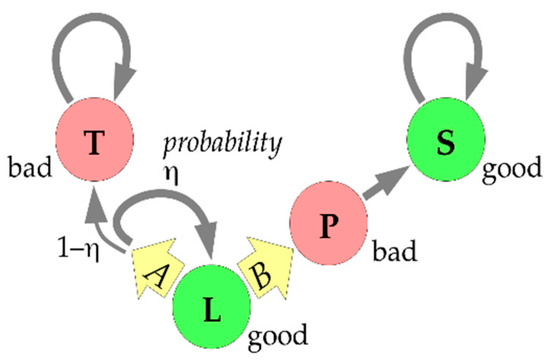
Figure 1.
Formal version of the thought experiment. A generation in the good state “L” can choose path “B”, surely leading to the good state “S” via the bad state “P” within two generations, or path “A”, probably keeping them in “L”, but possibly leading to the bad state “T”.
The main purpose of this narrative is not to add detail to the TE, but only to make it more accessible by suggesting a possible alternative interpretation of the states and options in the experiment that is simpler than the actual application to humanity and the Earth system that we motivated it with originally in the introduction. As any such narrative contains details that are not central to the problem one wants to study, but which might distract the analysis, the existence of two alternative narratives may also be used to check which aspects of them are actually crucial elements of the TE (namely those occurring in both narratives) and which are not. While the following text may sometimes refer to either narrative, our analysis will only depend on the formal specification.
Now why did we choose the specific formal specification above? The main justification is that it is essentially the form the potential decision dilemma between adaptation/growth and mitigation sketched in the introduction takes when one uses the recently developed theory of the state-space (rather than geographic) topology of sustainable management (TSM, [17]) to analyze a conceptual model of long-term climate and economic development [18].
TSM is a classification of the possible states of a dynamical system (such as the coupled system of natural Earth and humans on it) which has both a default dynamics (which it will display without the interference of an assumed “decision-maker” or “manager” such as a fictitious world government) and a number of alternative, “managed” dynamics (which the decision-maker may bring about by making certain “management” choices). The TSM classification starts with such a system and a set of possible states considered “desirable”, and then classifies each possible system state with regard to questions, such as “is this state desirable”, “will the state remain desirable by default/by suitable management”, “can a desirable state be reached with/without leaving the desirable region”, etc. This results in a number of state space regions that differ qualitatively w.r.t. the possibility of sustainable management. One of the most important among these state space regions is what is called a “lake” in TSM. In a “lake”, the decision-maker faces the dilemma of either (i) moving the system into an ultimately desirable and secure region called a “shelter”, but having to cross an undesirable region to do so; or (ii) using suitable management to avoid ever entering the undesirable region as long as management is sustained, but knowing that the system will enter the undesirable region when management is stopped, which leaves a permanent risk and makes the lake region insecure. Rather than giving the mathematical details of TSM (see [17] for those), let us exemplify these notions with a simple model of long-term climate and economic development, which was analyzed with TSM in [18].
The “AYS” model is a very simple conceptual model of long-term global climate and economic development, describing the deterministic development of just three aggregate continuous variables in continuous time via the ordinary differential equations:
with the auxiliary quantities:
dA/dt = E − A/τA
dY/dt = (β − θ A) Y
dS/dt = R − S/τS
E = F/ϕ, F = G U, R = (1 − G) U, U = Y/ε, G = 1/(1 + (S/σ)ρ).
In this, A is the excess atmospheric carbon stock over preindustrial levels, naturally decaying towards zero at rate τA but growing due to emissions E; Y is the gross world economic product, growing at a basic rate β slowed by climate-related damages; θ is the sensitivity of this slowing to A; S is the global knowledge stock for producing renewable energy, decaying at rate τS, but growing due to learning-by-doing in proportion to produced renewable energy R; energy efficiency ε stays constant so that total energy use, U, is proportional to Y; energy is supplied by either fossils, F, or renewables, R, in proportions depending on relative price G; σ is the break-even level of S at which fossils and renewables cost the same; ρ is a learning curve exponent; and, finally, emissions are proportional to fossil combustion with combustion efficiency ϕ.
In [18], several things are shown about this model system: (i) with plausible estimates of the initial state and parameters, it will eventually both violate the climate planetary boundary and stay at welfare levels below current welfare, converging to a fixed point with S = 0; (ii) The system can be forced to neither violate the climate planetary boundary nor to decrease welfare below current levels if humanity has the option to adjust the economic growth rate in real-time within some reasonable levels, but will return to case (i) once this management is stopped; and (iii) if one does not wait too long, it can also be forced to an alternative attractor where S and Y grow indefinitely if humanity can reduce σ by subsidizing renewables or taxing fossils to a reasonable extent, and this management can be phased-out some time after fossils have become uncompetitive, but this decarbonization transition cannot avoid decreasing welfare below current levels for a small number of generations.
In terms of the TSM classification, the attractor where the variables S and Y grow indefinitely lies in a “shelter” region where no management is necessary, and it corresponds to the TE’s state “S”. The initial state turns out to be in a “lake” region and corresponds to the TE’s state “L”, while the region one has to cross to reach the shelter from the lake is the state “P” (passage) in the TE. The permanently-managed alternative attractor at which S = 0 corresponds to what TSM calls a “backwater” from which the shelter can no longer be reached. The default attractor with thee planetary boundary and welfare boundary violated is either in what TSM calls a “dark downstream” region since one may still reach the backwater by management, or, if management options have broken down forever, it is in a “trench” region where no escape is possible any longer. If no management is used, the system will move from the lake to the dark downstream which becomes a trench when the management option is removed. In designing our TE, we omitted the dark downstream and simplified the situation so that the system directly goes to the trench (“T”) when management breaks down in “L”.
3. Analyses Using Rationality-Based Frameworks
We will now start to analyze the ethical aspects of the TE by applying a number of well-established frameworks based on a common assumption of rationality, where we take a broad working definition of rationality here that considers a decision-maker’s choice as rational if the decision-maker knows of no alternative choice that gives her a strictly more-preferred prospect than the choice taken, in view of her knowledge, beliefs, and capabilities.
Since we want to focus on what is the ethically right response to the dilemma rather than what makes a politically feasible or implementable choice, we will first treat humanity as a whole as formally just one single infinitely-lived decision-maker that perfectly knows the system as specified in the formal version of the TE, can make a new choice at every generation, can employ randomization for this if desired, can plan ahead, and has the overall goal of having high welfare in all generations. The natural framework for this kind of problem is the language of optimal control theory. Since it will turn out that optimal choices and plans (called “policies” in that language) will very much depend on the evaluation of trajectories (sequences of states) in terms of desirability, we will use concepts such as time preferences, inequality aversion, and risk aversion from decision theory and welfare economics to derive candidate intergenerational welfare functions to be used for this evaluation, and will discuss their impact on the optimal policy. We will restrict our analysis to a consequentialist point of view that takes into account only the actual and potential consequences of actions and their respective probabilities, and leave the inclusion of non-consequentialist, e.g., procedural [19], preferences for later work.
After that, we will refine the analysis by considering each generation a new decision-maker, so that humanity can no longer plan its own future choices, but rather a generation can only recommend and/or anticipate later generations’ choices. The natural framework for this kind of problem is the language of game theory. While most of economic theory applies game theory to selfish players, we will apply it instead to players with social preferences based on welfare measures since, in our TE, a generation’s welfare is deliberately assumed to be independent of their own choice between A and B.
3.1. Optimal Control Framework with Different Intergenerational Welfare Functions
3.1.1. Terminology
A trajectory, X, is a sequence of states X(0), X(1), … in the set {L, T, P, S}, where X(t) specifies the state generation t will be in. The only possible trajectories in our TE are
- “XcLT” = (L, …, L, T, T, …), with c > 0 times L and then T forever (so that c is the time of “collapse”);
- “XkLPS” = (L, …, L, P, S, S, …), with k > 0 times L, then once P, then S forever; and
- “all-L” = (L, L, …), which is possible, but has a probability of zero.
A reward sequence (RS, sometimes also called a payoff stream), denoted r, is a sequence r(0), r(1), r(2), … in the set {0, 1}, where r(t) = 0 or 1 means generation t has low or high overall welfare, respectively. Each trajectory determines an RS via r(t) = 1 if X(t) in {L, S} and r(t) = 0 otherwise. The only possible RSs are, thus:
- “rc10” = (1, …, 1, 0, 0, …) with c > 0 ones and then zeros forever;
- “rk101” = (1, …, 1, 0, 1, 1, …) with k > 0 ones, then one zero, then ones forever; and
- “all-1” = (1, 1, …), which is possible, but has a probability of zero.
A (randomized) policy (sometimes also called a strategy) from time 0 on, denoted as p, is just a sequence of numbers p(0), p(1), p(2), … in the interval [0, 1], where p(t) specifies the probability with which generation t will choose option A (staying in L) if they are in state L, i.e., if X(t) = L. In view of the possible trajectories, we may, without loss of generality, assume that if p(t) = 0 for some t, all later entries are irrelevant since state L will never occur after generation t. Thus, we consider only policies of the form:
- infinite sequences (p(0), p(1), …) with all p(t) > 0,
- finite sequences (p(0), p(1), …, p(k − 1), 0) with p(t) > 0 for all t < k.
The two most extreme (“polar”) policies are:
- “all-A” = (1, 1, …),
- “directly-B” = (0),
and another interesting set of policies is:
- “Bk” = (1, 1, …, 1, 0) with k + 1 ones, where the case k = 0 is “directly-B” and k → ∞ is “all-A”,
all of which are deterministic. A policy p is time-consistent iff it is a Markov policy, i.e., if and only if all its entries p(t) are equal, so the only time-consistent policies are “all-A”, “directly-B”, and the policies:
- “Ax” = (x, x, x, …) with 0 < x < 1, where the case x → 0 is “directly-B” and x → 1 is “all-A”.
Given a policy p, the possible trajectories and RSs have these probabilities:
- P(XcLT|p) = P(rc10|p) = p(0) η p(1) η … p(c − 2) η p(c − 1) π
- P(XkLPS|p) = P(rk101|p) = p(0) η p(1) η … p(k − 2) η (1 − p(k − 1))
- P(all-L|p) = P(all-1|p) = 0
Thus, each policy p defines a probability distribution over RSs, called a reward sequence lottery (RSL) here, denoted as RSL(p).
The only missing part of our control problem specification is now a function that numerically evaluates RSLs, or some other information on what RSLs are preferred over which others, in a way that allows the derivation of optimal policies. Let us assume we have specified a binary social preference relation that decides for each pair of RSLs g, h which of the following four cases holds: (i) g is strictly better than h, denoted as g > h; (ii) the other way around, h > g; (iii) they are equally desirable, g ~ h; or (iv) they are incomparable, denoted as g|h. We use the abbreviation g ≥ h for g > h or g ~ h, and g ≤ h for g < h or g ~ h. For example, we might put g > h iff V(g) > V(h) and g ~ h iff V(g) = V(h) for some evaluation function V.
Let us assume the social preference relation has the “consistency” property that each non-empty set C of RSLs contains some g such that h > g for no h in C. Then for each non-empty set C of policies, we can call any policy p in C optimal under the constraint C (or C-optimal for short) iff RSL(q) > RSL(p) for no q in C. In particular, if the preference relation encodes ethical desirability, C contains all policies deemed ethically acceptable, and p is C-optimal, then generation 0 has a good ethical justification in choosing option A with probability p(0) and option B with probability 1 − p(0).
We will now discuss several such preference relations and the resulting optimal policies. A common way of assessing preferences over lotteries is by basing them on preferences over certain outcomes, hence, we first consider whether each of two certain RSs, r and s, is preferable. A minimal plausible preference relation is based only on the Pareto principle that r(t) ≥ s(t) for all t should imply r ≥ s, and r(t) ≥ s(t) for all t but r(t) > s(t) for some t should imply r > s. In our case, the only strict preferences would then be between the RSs “all-1”, “rk101”, “rc10”, and “rc’10” for c > c’, where we would have “all-1” > “rk101” > “rc10” > “rc’10”. However, this does not suffice to make policy decisions, e.g., when we just want to compare policies “directly-B” with “all-A”, we need to compare RS “rk101” for k = 1 with a lottery over RSs of the form “rc10” for all possible values of c.
One possible criterion for preferring r over s is their degree of “sustainability”. The literature contains several criteria by which the sustainability of an RS could be assessed (see [20] for a detailed discussion). The maximin criterion (also known as the Rawlsian rule) focuses on the lowest welfare level occurring in an RS, which in all our cases is 0, hence, this criterion does not help in distinguishing options A and B. The satisfaction of basic needs criterion [21] asks from what time on welfare stays above some minimal level; if we use 1 as that level, this criterion prefers RS (1, 0, 1, 1, …) to all other RS that can occur with positive probability in our TE, hence, it will recommend policy “directly-B”, since it makes sure that generation 2 on welfare stays high. The overtaking and long-run average criteria [21] consider all RSs “rk101” equivalent and strictly more sustainable than all RSs “rc10”, hence, they also recommend “directly-B” since that is the only policy avoiding permanently low welfare for sure. Other sustainability criteria are based on the idea of aggregating welfare over time, which we will discuss next.
3.1.2. Aggregation of Welfare over Time
Let us now focus on the simple question whether the RS “rB” = (1, 0, 1, 1, …) that results from “directly-B” is preferable to the RS “rc10” = (1, 1, …, 1, 0, 0, …) with c ones, which may result from “all-A”? This may be answered quite differently. The easy way out is to deem them incomparable since, for some time points t, rB(t) > rc10(t), while for other t, rc10(t) > rB(t), but this does not help. A strong argument is that “rB” should be preferred since it has the larger number of generations with high welfare. Still, at least economists would object that real people’s evaluations of future prospects are typically subject to discounting, so that a late occurrence of low welfare would be considered less harmful than an early one. A very common approach in welfare economics is, therefore, to base the preference over RSs on some quantitative evaluation v(r), called an intergenerational welfare function, which in some way “aggregates” the welfare levels in r and can then also be used as a basis of an evaluation function V(g) of RSLs, which further aggregates the evaluations of all possible RSs in view of their probability. However, let us postpone the consideration of uncertainty for now and stick with the two deterministic RSs “rB” and “rc10”.
The most commonly used form of discounting (since it can lead to time-consistent choices) is exponential discounting, which would make us evaluate any RS r as:
using powers of a discount factor 0 ≤ δ < 1 that encodes humanity’s “time preferences”. For the above “rB” and “rc10”, this gives v(rB) = (1 − δ + δ²)/(1 − δ) and v(rc10) = (1 − δc)/(1 − δ). Thus, with exponential discounting, “rB” > “rc10” iff 1 − δ + δ² > 1 − δc or, equivalently, δc−1 + δ > 1, i.e., the policy “directly-B” is preferable iff δ is large enough or c is small enough. Since 1/δ can be interpreted as a kind of (fuzzy) evaluation time horizon, this means that “directly-B” will be preferable iff the time horizon is large enough to “see” the expected ultimate transition to state T at time c under the alternative extreme policy “all-A”. At what δ exactly the switch occurs depends on how we take into account the uncertainty about the collapse time c, i.e., how we get from preferences over RSs to preferences over RSLs, which will be discussed later. A variant of the above evaluation v due to Chichilnisky [21] adds to v(r) some multiple of the long-term limit, limt→∞ r(t), which is 1 for “rB” and 0 for all “rc10”, thus making “directly-B” preferable also for smaller δ, depending on the weight given to this limit.
v(r) = r(0) + δ r(1) + δ² r(2) + δ³ r(3) + …,
Let us shortly consider the alternative policy “Bk” = (1, …, 1, 0) with k ones, where choosing B is delayed by k periods, and “B1” equals “directly-B”. If k < c, this results in RS r(k + 1)101, which is evaluated as (1 − δk+1 + δk+2)/(1 − δ), which grows strictly with growing k. Thus, if the collapse time c was known, the best policy among the “Bk” would be the one with k = c − 1, i.e., initiating the transition at the last possible moment right before the collapse, which is evaluated as (1 − δc + δc+1)/(1 − δ) > (1 − δc)/(1 − δ), hence, it would be preferred to “all-A”. However, c is, of course, not known, but a random variable, so we need to come back to this question when discussing uncertainty below.
An argument against exponential discounting is that even for values of δ close to 1, late generations’ welfare would be considered too unimportant. Under the most common alternative form of discounting, hyperbolic discounting, one would instead have the evaluation:
v(r) = r(0) + r(1)/(1 + κ) + r(2)/(1 + 2κ) + r(3)/(1 + 3κ) + …
with some positive constant κ. Hyperbolic discounting can easily be motivated by an intrinsic suspicion that, due to factors unaccounted for, the expected late rewards may not actually be realized, but that the probability of this happening is unknown and has to be modeled via a certain prior distribution [22]. Under hyperbolic discounting, v(rB) is infinite while v(rc10) is finite independently of k, so the policy “directly-B” would always be preferable to “all-A” no matter how uncertainty about the actual c is accounted for.
A somewhat opposite alternative to hyperbolic discounting is what one could call “rectangular” discounting: simply average the welfare of only a finite number, say H many, of the generations:
v(r) = (r(0) + … + r(H − 1))/H,
where H is the evaluation horizon. With this, v(rB) = (H − 1)/H and v(rc10) = min(c, H)/H, so that v(rB) > v(rc10) iff H > c + 1. Thus, again, “directly-B” is preferable if the horizon is large enough.
3.1.3. Social Preferences over Uncertain Prospects: Expected Probability of Regret
Let us now consider evaluations of RSLs rather than RSs, which requires us to take into account the probabilities of all possible RSs that an RSL specifies.
If we already have a social preference relation “≥” on RSs, such as one of those discussed above, then a very simple idea is to consider an RSL g’’ strictly preferable to another RSL g’ iff the probability that a realization r’’(g’’) of the random process g’’ is strictly preferable to an independent realization r’(g’) of the random process g’ is strictly larger than ½:
g’’ > g’ iff P(r’’(g’’) > r’(g’)) > ½.
The rationale for this is based in the idea of expected probability of regret. Assume policy p was chosen, resulting in some realization r(RSL(p)), and someone asks whether not policy q should have been taken instead and argues that this should be evaluated by asking how likely the realization r’(RSL(q)) under the alternative policy would have been strictly preferable to the actual realization r(RSL(p)). Then the probability of the latter, averaged over all possible realizations r(RSL(p)) of the policy actually taken, should be not too large. This expected probability of regret is just P(r’’(g’’) > r’(g’)) for g’ = RSL(p) and g’’ = RSL(q). Since for the special case where g’ = g’’, the value P(r’’(g’’) > r’(g’)) can be everything up to at most ½, the best we can hope for is that P(r’’(RSL(q)) > r’(RSL(p))) ≤ ½ for all q ≠ p if we want to call p optimal.
In our example, the polar policy “directly-B” results in an RSL “gB” which gives 100% probability to RS “rB”, the opposite polar policy “all-A” results in an RSL “gA” which gives a probability of ηc−1π to RS “rc10”, and other policies result in RSLs with more complicated probability distributions. e.g., with exponential discounting, rB > rc10 iff δc−1 + δ > 1, hence, “gB” > “gA” iff the sum of ηc−1π over all c with δc−1 + δ > 1 is larger than ½. If c(δ) is the largest such c, which can be any value between 1 (for δ → 0) and infinity (for δ → 1), that sum is 1 − ηc(δ), which can be any value between π (for δ → 0) and 1 (for δ → 1). Similarly, with rectangular discounting, “rB” > “rc10” iff H > c + 1, hence, “gB” > “gA” iff 1 − ηH−1 > ½. In both cases, if η < ½, “directly-B” is preferred to “all-A”, while for η > ½, it depends on δ or H, respectively. In contrast, under hyperbolic discounting, “directly-B” is always preferred to “all-A”.
What about the alternative policy “Bk” as compared to “all-A”? If c ≤ k, we get the same reward sequence as in “all-A”, evaluated as (1 − δc)/(1 − δ). If c > k, we get an evaluation of (1 − δk+1 + δk+2)/(1 − δ), which is larger than (1 − δc)/(1 − δ) iff δc−k−1 + δ > 1. Thus, RSL(Bk) > gA iff the sum of ηc−1π over all c > k with δc−k−1 + δ > 1 is larger than ½. Since the largest such c is c(δ) + k, that sum is ηk(1 − ηc(δ)), so whenever “Bk” is preferred to “all-A”, then so is “directly-B”. Let us also compare “Bk” to “directly-B”. In all cases, “directly-B” gets (1 − δ + δ2)/(1 − δ), while “Bk” gets the larger (1 − δk+1 + δk+2)/(1 − δ) if c > k, but only (1 − δc)/(1 − δ) if c ≤ k. The latter is < (1 − δ + δ2)/(1 − δ) iff c ≤ c(δ). Thus, “directly-B” is strictly preferred to “Bk” iff 1 − ηmin(c(δ),k) > ½, i.e., iff both c(δ) and k are larger than log(½)/log(η), which is at least fulfilled when η < ½. Conversely, “Bk” is strictly preferred to “directly-B” iff either c(δ) or k is smaller than log(½)/log(η). In particular, if social preferences were based on the expected probability of regret, delaying the choice for B by at least one generation would be strictly preferred to choosing B directly whenever η > ½, while at the same time, delaying it forever would be considered strictly worse at least if the time horizon is long enough. Basing decisions on this maxim would, thus, lead to time-inconsistent choices: in every generation, it would seem optimal to delay the choice B by the same positive number of generations, but not forever, so no generation would actually make that choice.
Before considering a less problematic way of accounting for uncertainty, let us shortly discuss a way of deriving preferences over RSs rather than RSLs that is formally similar to the above. In that case the rationale would not be in terms of regret but in terms of Rawls’ veil of ignorance. Given two RSs r’ and r’’, would one rather want to be born into a randomly selected generation in situation r’ or into a randomly selected generation in situation r’’? i.e., let us put:
r’’ > r’ iff P(r’’(t’’) > r’(t’)) > ½,
where t’’, t’ are drawn independently from the same distribution, e.g., the uniform one on the first H generations or a geometric one with parameter δ. Then rB(t’’) > rc10(t’) iff rB(t’’) = 1 and rc10(t’) = 0, i.e., iff t’’ ≠ 1 and t’ > c. Under the uniform distribution over H generations, the latter has a probability of (H − 1)(H − c)/H² if H ≥ c, which can be any value between 0 (for H = c) and 1 (for very large H), hence, whether “rB” > “rc10” depends on H again. Similarly, rB(t’’) < rc10(t’) iff rB(t’’) = 0 and rc10(t’) = 1. This has probability min(c,H)/H², which is 1 for H = 1 and approaches 0 for very large H, hence, whether “rB” < “rc10” depends on H as well. However, this version of preferences over RS leaves a large possibility for undecidedness, “rB”|“rc10”, where neither “rB” > “rc10” nor “rc10” > “rB”. This is the case when both (H − 1)(H − c)/H² and min(c,H)/H² are at most ½, i.e., when max[(H − 1)(H − c), min(c,H)] ≤ H²/2, which is the case when H ≥ 2 and H² − 2(c + 1)H + 2c ≤ 0, i.e., when 2 ≤ H ≤ c + 1 + (c² + 1)½. A similar result holds for the geometric distribution with parameter δ. Thus, while the probability of regret idea can lead to time-inconsistent choices, the formally similar veil of ignorance idea may not be able to differentiate enough between choices. Another problematic property of our veil of ignorance-based preferences is that they can lead to preference cycles. e.g., assume H = 3 and compare the RSs r = (0, 1, 2), r’ = (2, 0, 1), and r’’ = (1, 2, 0). Then it would occur that r > r’ > r’’ > r, so there would be no optimal choice among the three.
3.1.4. Evaluation of Uncertain Prospects: Prospect Theory and Expected Utility Theory
We saw that the above preference relations based on regret and the veil of ignorance, while intuitively appealing, are, however, unsatisfactory from a theoretical point of view, since they can lead to time-inconsistent choices and preference cycles, i.e., they may fail to produce clear assessments of optimality. The far more common way of dealing with uncertainty is, therefore, based on numerical evaluations instead of binary preferences. A general idea, motivated by a similar theory regarding individual, rather than social, preferences, called prospect theory [23], is to evaluate an RSL g by a linear combination of some function of the evaluations of all possible RSs r with coefficients that depend on their probabilities:
V(g) = ∑r w(P(r|g)) f(v(r)).
In the simplest version, corresponding to the special case of expected utility theory, both the probability weighting function w and the evaluation transformation function f are simply the identity, w(p) = p and f(v) = v, so that V(g) = ∑r P(r|g) v(r) = Eg v(r), the expected evaluation of the RSs resulting from RSL g. If combined with a v(r) based on exponential discounting, this gives the following evaluations of our polar policies:
V(RSL(directly-B)) = v(rB) = (1 − δ + δ²)/(1 − δ)
and:
V(RSL(all-A)) = Eall-A v(rc10) = ∑c>0 ηc−1π(1 − δc)/(1 − δ) = 1/(1 − δη).
Hence, “directly-B” is preferred to “all-A” iff (1 − δ + δ²)(1 − ηδ) − 1 + δ > 0. Again, this is the case for δ > δcrit(η) with δcrit(0) = 0 and δcrit(1) = 1. The result for rectangular discounting is similar, while for hyperbolic discounting “directly-B” is always preferred to “all-A”, and all of this as expected from the considerations above.
In prospect theory, the transformation function f can be used to encode certain forms of risk attitudes. For example, we could incorporate a certain form of risk aversion against uncertain social welfare sequences by using a strictly concave function f, such as f(v) = v1−a with 0 < a < 1 (isoelastic case) or f(v) = −exp(−av) with a > 0 (constant absolute risk aversion) (welfare economists might be confused a little by our discussion of risk aversion since they are typically applying the concept in the context of consumption, income or wealth of individuals at certain points in time, in which context one can account for risk aversion already in the specification of individual consumers’ utility function, e.g., by making utility a concave function of individual consumption, income, or wealth. Here we are, however, interested in a different aspect of risk aversion, where we want to compare uncertain streams of societal welfare rather than uncertain consumption bundles of individuals. Thus, even if our assessment of the welfare of each specific generation in each specific realization of the uncertainty about the collapse time c already accounts for risk aversion in individual consumers in that generation, we still need to incorporate the possible additional risk aversion in the “ethical social planner”). This basically leads to a preference for small variance in v. One can see numerically that in both cases increasing the degree of risk aversion, a, lowers δcrit(η), not significantly so in the isoelastic case but significantly in the constant absolute risk aversion case, hence, risk aversion favors “directly-B”. In particular, the constant absolute risk aversion case with a → ∞ is equivalent to a “worst-case” analysis that always favors “directly-B”. Conversely, one can encode risk-seeking by using f(v) = v1+a with a > 0.
Under expected utility theory, the delayed policy “Bk” has:
(1 − δ) × V(RSL(Bk)) = ηk(1 − δk+1 + δk+2) + ∑c=1…k ηc−1π(1 − δc),
which is either strictly decreasing or strictly increasing in k. Since “directly-B” and “all-A” corresponds to the limits k → 0 and k → ∞, “Bk” is never optimal but always worse than either “directly-B” or “all-A”. The same holds with risk-averse specifications of f. Under isoelastic risk-seeking with f(v) = v1+a, however, we have:
which may have a global maximum for a strictly positive and finite value of k, so that delaying may seem preferable. e.g., with δ = 0.8, η = 0.95, and a = ½, V(RSL(Bk)) is maximal for k = 6, i.e., one would want to choose six times A before choosing B, again a time-inconsistent recommendation.
(1 − δ) × V(RSL(Bk)) = ηk(1 − δk+1 + δk+2)1+a + ∑c=1…k ηc−1π(1 − δc)1+a,
As long as the probability weighting function w is simply the identity, there is always a deterministic optimal policy. While other choices for w could potentially lead to non-deterministic optimal policies, they can be used to encode certain forms of risk attitudes that cannot be encoded via f. e.g., one can introduce some degree of optimism or pessimism by over- or underweighing the probability of the unlikely cases where c is large. For example, if we put w(p) = p1−b with 0 ≤ b < 1, then increasing the degree of optimism b, one can move δcrit(η) arbitrarily close towards 1, which is not surprising. We will however not discuss this form of probability reweighting further but will use a different way of representing “caution” below. Since that form is motivated by its formal similarity to a certain form of inequality aversion, we will discuss the latter first now before returning to risk attitudes.
3.1.5. Inequality Aversion: A Gini-Sen Intergenerational Welfare Function
While discounting treats different generations’ welfare differently, it only does so based on time lags, and all the above evaluations still only depend on some form of (weighted) time-average welfare and are blind to welfare inequality as long as these time-averages are the same. However, one may argue that an RS with less inequality between generations, such as (1, 1, 1, …), should be strictly preferable to one with the same average but more inequality, such as (2, 0, 2, 0, 2, 0, …). Welfare economics has come up with a number of different ways to make welfare functions sensitive to inequality, and although most of them were initially developed to deal with inequality between individuals of a society at a given point in time (which we might call “intragenerational” inequality here), we can use the same ideas to deal with inequality between welfare levels of different generations (“intergenerational” inequality). Since our basic welfare measure is not quantitative but qualitative since it only distinguishes “low” from “high” welfare, inequality metrics based on numerical transformations, such as the Atkinson-Theil-Foster family of indices, are not applicable in our context, but the Gini-Sen welfare function [24], which only requires an ordinal welfare scale, is. The idea is that the value of a specific allocation of welfare to all generations is the expected value of the smaller of the two welfare values of two randomly-drawn generations. If the time horizon is finite, H > 0, this leads to the following evaluation of an RS r:
V2(r) = (∑t=0…H−1 ∑t’=0…H−1 min[r(t), r(t’)])/H².
It is straightforward to generalize the idea from drawing two to drawing any integer number a > 0 of generations, leading to a sequence of welfare measures Va(r) that get more and more inequality averse as a is increased from 1 (no inequality aversion, “utilitarian” case) to infinity (complete inequality aversion), where the limit for a → ∞ is the egalitarian welfare function:
V1(r) = [r(0) + … + r(H − 1)]/H
Va(r) = (∑t1=0…H−1 … ∑ta=0…H−1 min[r(t1), …, r(ta)])/Ha
V∞(r) = min[r(0), …, r(H − 1)]
Note that I = 1 − V2(r)/V1(r) is the Gini index of inequality and the formula V2(r) = V1(r) (1 − I) is often used as the definition of the Gini-Sen welfare function.
Our RSs “rc10” then gets Va(rc10) = min(c/H, 1)a, while “rk101” gets Va(rk101) = [(H − 1)/H]a if k < H and Va(rk101) = 1 if k ≥ H. Together with expected utility theory for evaluating the risk about c, this makes:
and Va(directly-B) = [(H − 1)/H]a. Numerical evaluation shows that even for large H, “all-A” may still be preferred due to the possibility that collapse will not happen before H and all generations will have the same welfare, but this is only the case for extremely large values of a. If we use exponential instead of rectangular discounting and compare the policies “directly-B”, “Bk”, and “all-A”, we may again get a time-inconsistent recommendation to choose B after a finite number of generations. e.g., Figure 2a shows V(Bk) vs. k for the case η = 0.985, δ = 0.9, a = 2, where the optimal delay would appear to be five generations. If we restrict our optimization to the time-consistent policies “Ax”, the optimal x in that case would be ≈0.83, i.e., each generation would choose A with about 83% probability and B with about 17% probability, as shown in Figure 2b. Still, note that the absolute evaluations vary only slightly in this example.
Va(all-A) = ηH + ∑c=1…H ηc−1π(c/H)a
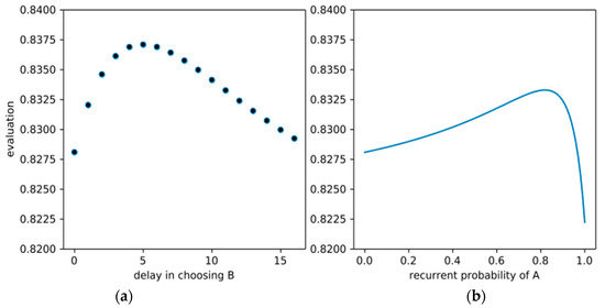
Figure 2.
Inequality-averse evaluation of deterministic but delayed policies (a) and time-consistent but probabilistic policies (b) for the case η = 0.985, δ = 0.9 and a = 2.
Let us see what effect a formally similar idea has in the context of risk aversion.
3.1.6. Caution: Gini-Sen Applied to Alternative Realizations
What happens if instead of drawing a ≥ 1 many generations t1, …, ta at random, we draw a ≥ 1 many realizations r1, …, ra of an RSL g at random and use the expected minimum of all the RS-evaluations V(ri) as a “cautious” evaluation of the RSL g?
Va(g) = ∑r1 … ∑ra g(r1) × … × g(ra) × min[v(r1), …, v(ra)].
For a = 1, this is just the expected utility evaluation of g, while for a → ∞, it gives a “worst-case” evaluation. For actual numerical evaluation, the following equivalent formula is more useful (assuming that all v(r) ≥ 0):
Va(g) = ∫x≥0 Pg(v(r) ≥ x)a dx,
where Pg(v(r) ≥ x) is the probability that v(r) ≥ x if r is a realization of g. In that form, a can be any real number ≥ 1 and it turns out that the evaluation is a special case of cumulative prospect theory [23], with the cumulative probability weighting function w(p) = pa. Focusing on “all-A” vs. “directly-B” again, we get Va(all-A) = (1 − ηaH)/(1 − ηa)H and Va(directly-B) = (H − 1)/H, hence, “all-A” is preferred iff (1 − ηaH)/(H − 1) > 1 − ηa, i.e., iff H and a are small enough and η is small enough. In particular, regardless of H and η, for a → ∞ we always get a preference for “directly-B” as in the constant absolute risk aversion. This is because with the Gini-Sen-inspired specification of caution, the degree of risk aversion effectively acts as an exponent to the survival probability η, i.e., increasing risk aversion has the same effect as increasing collapse probability, which is an intuitively appealing property.
3.1.7. Fairness as Inequality Aversion on Uncertain Prospects
Consider the RSs r1 = (1, 0, 1) and r2 = (1, 1, 0), and the RSL g that results in r1 or r2 with equal probability ½. If we apply inequality aversion on the RS level as above, say with a = 2, we get V(r1) = V(r2) = V(g) = 4/9. Still, g can be considered more fair than both r1 and r2 since under g, the expected rewards are (1, ½, ½) rather than (1, 0, 1) or (1, 1, 0), so no generation is doomed to zero reward but all have a fair chance of getting a positive reward. It is, therefore, natural to consider applying “inequality aversion” on the RSL level to encode fairness, by putting:
where V(g, t) is some evaluation of the uncertain reward of generation t resulting from g, e.g., the expected reward or some form of risk-averse evaluation. The interpretation is that Va(g) is the expected minimum of how two randomly drawn generations within the time horizon evaluate their uncertain rewards under g. Using exponential discounting instead, the formula becomes:
Va(g) = (∑t1=0…H−1 … ∑ta=0…H−1 min[V(g, t1), …, V(g, ta)])/Ha,
Va(g) = (1 − δ)a ∑t1=0…H−1 … ∑ta=0…H−1 δt1+...+ta min[V(g, t1), …, V(g, ta)].
If we use the expected reward for V(g, t) and evaluate the time-consistent policies “Ax” with this Va(g), the result looks similar to Figure 2b, i.e., the optimal time-consistent policy is again non-deterministic. A full optimization of Va(g) over the space of all possible probabilistic policies shows that the overall optimal policy regarding Va(g) is not much different from the time-consistent one, it prescribes choosing A with probabilities between 79% and 100% in different generations for the setting of Figure 2.
3.1.8. Combining Inequality and Risk Aversion with Fairness
How could one consistently combine all the discussed aspects into one welfare function? Since a Gini-Sen-like technique of using minima can be used for each of them, it seems natural to base a combined welfare function on that technique as well. Let us assume we want to evaluate the four simple RSLs g1, …, g4 listed in Table 1 in a way that makes V(g1) > V(g2) because the latter is more risky, V(g2) > V(g3) because the latter has more inequality, and V(g3) > V(g4) because the latter is less fair. Then we can achieve this by applying the Gini-Sen technique several times to define welfare functions V0 … V6 that represent more and more of our aspects as follows:

Table 1.
Comparison of the effects of inequality aversion, overall and generational risk aversion, and fairness on the evaluation of four simple reward sequence lotteries (RSLs). All effects are implemented in the Gini-Sen style (see main text for details), inequality aversion with a larger degree of a = 3, risk aversion and fairness with a lower degree of a = 2, which is reflected in the preference for the coin toss between the “no-inequality” reward sequences (0, 0) and (1, 1) over the coin toss between the “equal average” reward sequences (0, 1) and (1, 0).
- Simple averaging: V0(g) = Er Et r(t) where Er f(r) is the expectation of f(r) w.r.t. the lottery g and Et f(t) is the expectation of f(t) w.r.t. some chosen discounting weights;
- Gini-Sen welfare of degree a = 3: V1(g) = Er Et1 Et2 Et3 min{r(t1), r(t2), r(t3)};
- Overall risk-averse welfare: V2(g) = Er1 Er2 min{Et r1(t), Et r2(t)};
- Fairness-seeking welfare of degree a = 3: V3(g) = Et1 Et2 Et3 min{Er r(t1), Er r(t2), Er r(t3)};
- Inequality- and overall risk-averse welf.: V4(g) = Er1 Er2 min{v4(r1), v4(r2)} with v4(r) = Et1 Et2 Et3 min{r(t1), r(t2), r(t3)};
- Inequality and overall risk index: I4(g) = 1 − V4(g)/V0(g);
- Generational risk averse and fair welfare: V5(g) = Et1 Et2 Et3 min{V5(g, t1), V5(g, t2), V5(g, t3)} with V5(g, t) = Er1 Er2 min{r1(t), r2(t)};
- Generational risk and fairness index: I5(g) = 1 − V5(g)/V0(g); and
- All effects combined: V6(g) = V4(g)V5(g)/V0(g) = V0(g)[1 − I4(g)][1 − I5(g)]
The resulting evaluations for g1 … g4 can be seen in Table 1. We chose a higher degree of inequality-aversion (a = 3) than the degree of risk-aversion (a = 2) so that V6(g2) > V6(g3) as desired. Applied to our thought experiment, V6 can result in properly probabilistic and time-inconsistent policy recommendations, as shown in Figure 3 for two example choices of η and discounting schemes. An alternative way of combining inequality and risk aversion into one welfare function would be to use the concept of recursive utility [25], which is, however, beyond the scope of this article.
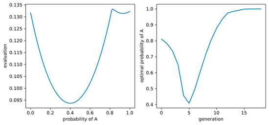
Figure 3.
(Left) Evaluation V6 for the case of η = 0.68, rectangular discounting with very short horizon 3 and choosing A for sure in generation 1, by probability of chosing A in generation 0, showing an optimal probability of approximately 82%. (Right) Optimal policy for the first 20 generations according to V6 for the case of η = 0.97 and exponential discounting with δ = 0.9.
Summarizing the results of our analysis in the optimal control framework that treats humanity as a single infinitely-lived decision-maker, we see that there is no clear recommendation to either choose A or B at time 0 since depending on the degrees and forms of time preferences/time horizon and risk/inequality/fairness attitudes, either one of the policies “all-A” or “directly-B” may appear optimal, or it may even appear optimal to deterministically delay the choice for B by a fixed number of generations or choose A by a time-varying probability, leading to time-inconsistent recommendations. At least we were able to formally confirm quite robustly the overall intuition that risk aversion and long time horizons are arguments in favor of B while risk seeking and short time horizons are arguments in favor of A. Only the effect of inequality aversion might be surprising, since it can lead to either recommending a time-inconsistent policy of delay (if we restrict ourselves to deterministic policies) or a probabilistic policy of choosing A or B with some probabilities (if we restrict ourselves to time-consistent policies). In the next subsection, we will see what difference it makes that no generation can be sure about the choices of future generations.
3.2. Game-Theoretical Framework
While the above analysis took the perspective of humanity as a single, infinitely lived “agent” that can plan ahead its long-term behavior, we now take the viewpoint of the single generations who care about intergenerational welfare, but cannot prescribe policies for future generations and have to treat them as separate “players” with potentially different preferences instead. For the analysis, we will employ game-theory as the standard tool for such multi-agent decision problems. Each generation, t, is treated as a player who, if they find themselves in state L, has to choose a potentially randomized strategy, p(t), which is, as before, the probability that they choose option A. Since each generation is still assumed to care about future welfare, the optimal choice of p(t) depends on what generation t believes future generations will do if in L. As usual in game theory, we encode these beliefs by subjective probabilities, denoting by q(t’, t) the believed probability by generation t’ that generation t > t’ will choose A when still in L.
Let us abbreviate generation t’ by Gt’ and the set of generations t > t’ by G>t’ and focus on generation t’ = 0 at first. Let us assume that V = V4, V5, or V6 with exponential discounting encodes their social preferences over RSLs. Given G0′s beliefs about G>0′s behavior, q(0, t) for all t > 0, we then need to find that x in [0, 1] which maximizes V(RSL(px,q)), where px,q is the resulting policy px,q = (x, q(0, 1), q(0, 2), …). If G0 believes G1 will choose B for sure (i.e., q = (0, …) = “directly-B”) and chooses strategy x, the resulting RSL(px,q) produces the reward sequence r1 = (1, 0, 0, …) with probability xπ, r2 = (1, 0, 1, 1, …) with probability 1 − x, and r3 = (1, 1, 0, 1, 1, …) with probability xη. Hence:
V4(RSL(px,q)) =
x² [(1 − (1 − δ)δ²)³ η² − (1 − δ)³η² + 2(1 − δ)³η − 2(1 − (1 − δ)δ)³η − (1 − δ) + (1 − (1 − δ)δ)³]
+ 2x (−(1 − δ)³η + (1 − (1 − δ)δ)³η + (1 − δ)³ − (1 − (1 − δ)δ)³] + (1 − (1 − δ)δ)³.
x² [(1 − (1 − δ)δ²)³ η² − (1 − δ)³η² + 2(1 − δ)³η − 2(1 − (1 − δ)δ)³η − (1 − δ) + (1 − (1 − δ)δ)³]
+ 2x (−(1 − δ)³η + (1 − (1 − δ)δ)³η + (1 − δ)³ − (1 − (1 − δ)δ)³] + (1 − (1 − δ)δ)³.
Since the coefficient in front of x² is positive, V4 is maximal for either x = 0, where it is (1 − δ + δ²)³, or for x = 1, where it is (δ³ − δ² + 1)³η² + (δ − 1)³(η² − 1), which is always smaller, so w.r.t. V4, x = 0 (choosing B for sure) is optimal under the above beliefs. For V5, we have V5(RSL(px,q), t) = 1 for t = 0, (xη)² for t = 1, (1 − x)² for t = 2, and (1 − xπ)² for t > 2. If x < 1/(1 + η), we have (xη)² < (1 − x)² < (1 − xπ)² < 1, while for x > 1/(1 + η), we have (1 − x)² < (xη)² < (1 − xπ)² < 1. For x ≤ 1/(1 + η), V5(RSL(px,q)) is again quadratic in x with a positive x² coefficient with value 1 + (1 − δ)³ − (1 − δ²)³ at x = 0 and, again, a smaller value at x = 1/(1 + η). Additionally, for x ≥ 1/(1 + η), V5(RSL(px,q)) is quadratic in x with positive x² coefficient and a value of:
for x = 1, which is larger than the value for x = 0 if η is large enough and/or δ small enough. A similar thing holds for the combined welfare measure V6, as shown in Figure 4, blue line, for the case η = 0.95 and δ = 0.805, where G0 will choose A if they believe G1 will choose B, resulting in an evaluation V6 ≈ 0.43. The orange line in the same plot shows V6(RSL(px,q)) for the case in which G0 believes that G1 will choose A and G2 will choose B if they are still in L, which corresponds to the beliefs q = (1, 0, …). Interestingly, in that case, it is optimal for G0 to choose A, resulting in an evaluation V6 ≈ 0.42. Since the dynamics and rewards do not explicitly depend on time, the same logic applies to all later generations, i.e., for that setting of η and δ and any t ≥ 0, it is optimal for Gt to choose A when they believe Gt+1 will choose B and optimal to choose B when they believe Gt+1 will choose A and Gt+2 will choose B.
1 − δ(3 − 3δ + δ² − η²[1 − δ + δ²][3 − δ(1 − δ + δ²)(3 − δ + δ² − δ³)])
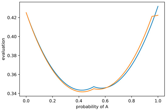
Figure 4.
Evaluation V6 for the case of η = 0.95 and δ = 0.805 depending on the first generation’s probability of choosing A (horizontal axis), for the case where they expect the next generations to choose B (blue line) or to choose A and then B (orange line).
Now assume that all generations have preferences encoded by welfare function V6 and believe that all generations Gt with even t will choose A and all generations Gt with odd t will choose B. Then it is optimal for all generations to do just that. In other words, these assumed common beliefs form a strategic equilibrium (more precisely, a subgame-perfect Nash equilibrium) for that setting of η and δ. However, under the very same set of parameters and preferences, the alternative common belief that all even generations will choose B and all odd ones A also forms such an equilibrium. Another equilibrium consists of believing that all generations choose A with probability ≈83.7% which all generations evaluate as only V6 ≈ 0.40, which is less than in the other two equilibria. The existence of more than one strategic equilibrium is usually taken as an indication that the actual behavior is very difficult to predict even when assuming complete rationality. In our case, this means G0 cannot plausibly defend any particular belief about G>0′s policy on the grounds of G>0′s rationality since G>0 might follow at least either of the three identified equilibria (or still others). In other words, for many values of η and δ a game-theoretic analysis based on subgame-perfect Nash equilibrium might not help G0 in deciding between A and B. A common way around this is to consider “stronger” forms of equilibrium to reduce the number of plausible beliefs, but this complex approach is beyond the scope of this article. An alternative and actually older approach [26] is to use a different basic equilibrium concept than Nash equilibrium, not assuming players have beliefs about other players policies encoded as subjective probabilities, but rather assuming players apply a worst-case analysis. In that analysis, each player would maximize the minimum evaluation that could result from any policy of the others. For choosing B, this evaluation is simply v(1, 0, 1, 1, …), while, for choosing A, the evaluation can become quite complex. Instead of following this line here, we will use a similar idea when discussing the concept of responsibility in the next section, where we will discuss other criteria than rationality and social preferences.
4. Solutions Based on Other Ethical Principles and Sustainability Paradigms
4.1. Responsibility
Rather than asking what combinations of uncertain welfare levels we should prefer for future generations, one can also ask what responsibility we have regarding future welfare. We will sketch here a certain simple theory of responsibility designed to be applicable to problems involving multiple agents, uncertainty, and potential ethically-undesired outcomes (EUOs), as in our TE. We distinguish two major types of responsibility, forward- and backward-looking responsibility, the latter having two subtypes, factual and counterfactual responsibility. While forward-looking responsibility is about still-existing possibilities, an agent or group of agents has to reduce the probability of future EUOs (“responsibility to”), backward-looking responsibility (“responsibility for”) is about past possibilities that would have reduced the probability of an EUO that actually occurred (factual responsibility, e.g., Nagel’s unlucky drunken driver [27]) or could have occurred (counterfactual responsibility, e.g., Nagel’s lucky drunken driver [27]). In all three types, the degree of responsibility is measured in terms of differences of probabilities of EUOs. Rather than giving a formal definition, it will suffice to discuss the details of this theory at the hand of several choices for what constitutes an EUO in our TE.
Let us start by considering that an EUO is simply a low welfare in generation 1. Then the degree of forward-looking respectively of G0 is the absolute difference between the probability of low welfare in generation 1 when choosing A rather than B, which equals η. In other words, G0 would have a degree of η responsibility to choose A in order to avoid the EUO that G1 gets low welfare. If they choose B instead, they will have a degree of factual backward-looking responsibility for G1′s low welfare equaling again η since this is the amount by which they could have reduced the probability of the EUO. If they behave “responsibly” by choosing A, G1′s welfare might also be low (with probability π), but G0 would still not have backward-looking responsibility since they could not have reduced that probability.
If the EUO was simply a low welfare in G2 rather than G1, the assessment of G0′s responsibility must consider the possible actions of G1 in addition to those of G0. If G0 chooses B, the probability of the EUO is zero, while if they choose A, it depends on G1′s choice. If G1 would choose B, the EUO has probability 1 so that G0′s choice would make a difference of 1, while if G1 would choose A, the EUO has probability 1 − η² < 1 and G0′s choice would make a difference of only 1 − η² < 1. In both cases, however, they have considerable forward-looking responsibility to choose B since by that they can reduce the probability of the EUO significantly. If choosing B, no backward-looking respectively accrues. If G0 and G1 both choose A and the collapse occurs at time 2, G1 has no factual responsibility since they could not have reduced that probability, but G0 has factual responsibility of degree 1 − η². If G0 chooses A and G1 B, G1′s factual responsibility is η as seen above, but G0′s is even larger, since in view of G1′s actual choice, G0 could have reduced the probability from one to zero by choosing B instead. Thus, G0 has factual responsibility of 1. It might seem counterintuitive at first that the sum of the factual responsibilities of the two agents regarding that single outcome would be larger than 100%, but our theory is actually explicitly designed to produce this result in order to show that responsibility cannot simply be divided. Otherwise, each individual in a large group of bystanders at a fight in public could claim to have almost no responsibility to intervene (diffusion of responsibility). Finally, if both G0 and G1 choose B and no collapse happens, G0 still has counterfactual responsibility since the collapse could have happened and G0 could have reduced that probability by 1 − η². This distinction between factual and counterfactual responsibility would also allow a discussion of Nagel’s concept of moral luck in consequences [27] and responses to it, such as [28] but we will not go there here.
If the EUO is low welfare in G3, it becomes more complicated. By choosing B, G0 can avoid the EUO for sure, but when choosing A they might hope G1 will choose B and the EUO will be avoided for sure as well, in which case they might claim to have a rather low responsibility to choose B which amounts only to π, the probability that G1 will have no chance of choosing B due to immediate collapse. Common sense, however, shows that while wishful thinking regarding the actions of others might affect one’s own psychological assessment of responsibilities, it cannot be the basis for an ethical observer’s assessment of responsibility. Otherwise, even in a group of just two bystanders, neither one would be ethically obliged to intervene since both could hope the other does. Here we even take the opposite view and argue that G0′s degree of forward-looking responsibility should equal the largest possible amount by which they might be able to reduce the probability of the EUO, maximized over all possible behaviors of the other agents. This means that rather than being optimistic about G1′s action, they need to be pessimistic about both G1′s and G2′s behavior. The worst that can happen regarding the welfare of G3 when G0 chooses A is that G1 would choose A and G2, B. In that case, the EUO has probability 1, so G0 would still be fully responsible (degree 1) to choose B in order to avoid the EUO.
Now what definition of EUO should we actually adopt in our TE? Two candidates seem natural, either a low welfare in any generation should already constitute an EUO (in which case it cannot be avoided by either A or B), or only an infinite number of low welfare generations, i.e., an eventual collapse into state T, should constitute an EUO. In the latter case, each generation in L has 100% forward-looking responsibility to choose B, and if they choose A instead, they will end up having 100% factual responsibility for the eventual collapse, regardless of the choices of later generations. Summarizing, we argue that a theory of responsibility that avoids the diffusion of responsibility and wishful thinking will deem B the responsible action in our TE since it avoids the worst for sure, even though this makes G0 responsible for G1′s suffering.
4.2. Safe Operating Space for Humanity
In the following we continue our analyses of the ethical aspects of the TE from the perspective of the safe operating space (SOS) for humanity [2]. The SOS is located within planetary boundaries (PBs) “with respect to the Earth system” which “are associated with the planet’s biophysical subsystems and or processes” [2]. The SOS is a fairly new concept for environmental governance, encapsulating several established concepts, such as the limits to growth [29,30], safe minimum standards [31,32,33], the precautionary principle [34], and the tolerable windows concept [35,36]. We let our analysis guide by the three “main” articles around the planetary boundaries and the SOS concepts [2,3,4], which have, at the time of this writing, together well over ten thousand citations, so that a comprehensive review of the SOS debate is beyond the possibilities of this article. We will, therefore, incorporate other papers only selectively.
One main difference to the approaches covered in the previous sections is the level of mathematical formalization. While we do acknowledge that some attempts of mathematical formalization of a SOS decision paradigm have been made [37], the original and most of the subsequent works do not provide a mathematical operationalization.
First of all we assess whether our TE is a suitable model within which the SOS concept can be applied at all. Rockström et al. [3] acknowledges that “anthropogenic pressures on the Earth System have reached a scale where abrupt global environmental change can no longer be excluded”, which “can lead to the unexpected crossing of thresholds that drive the Earth System, or significant sub-systems, abruptly into states deleterious or even catastrophic to human well-being”. Therefore, the authors “propose a new approach to global sustainability in which we define planetary boundaries within which we expect that humanity can operate safely.” These lines resemble very well the situation in our TE where the decision-maker faces either a transition from L to T or from L to S.
However, the authors of the three papers in question do not mention any unfavorable P-like states on the way from L to S. Rockström et al. [2] states that “the evidence so far suggests that, as long as the thresholds are not crossed, humanity has the freedom to pursue long-term social and economic development.“ Emphasizing the long-term aspect, the last quote at least does not exclude the possibility of unfavorable interim states P on the way to safe, long-term “shelter” states S.
Nevertheless, opposing to the view that the SOS can be applied to the decision problem in our TE, the planetary boundaries’ “precautionary approach is based on the maintenance of a Holocene-like state of the ES [Earth System]” [4]. This is emphasized because the “thresholds in key Earth System processes exist irrespective of peoples’ preferences, values or compromises based on political and socioeconomic feasibility, such as expectations of technological breakthroughs and fluctuations in economic growth.” [3]. One could argue that a mere transition from state L to S has to be interpreted as “destabilizing” [4]. However, this view disregards that our TE does not tell anything about the Holocene-likeness of the states L, T, P, and S. One may very well interpret states L, P, and S as Holocene-like. Further, as stated above, the ultimate justification for the planetary boundaries is to avoid Earth system states “catastrophic to human well-being” [3]. It is the only precautionary principle used by the PB approach that suggests staying within Holocene-like state.
Another opposition to the view that the SOS can be applied to the decision problem in our TE may result from the fact that “the planetary boundaries approach as of yet focuses on boundary definitions only and not as a design tool of compatible action strategies” [3]. The “PB framework as currently construed provides no guidance as to how […] the maintenance of a Holocene-like state […] may be achieved […] and it cannot readily be used to make choices between pathways for piecemeal maneuvering within the SOS or more radical shifts of global governance” [4]. We make two observations from these quotes: First, the PB framework may not be used to guide how Holocene-like states shall be maintained, but it can surely be used as a guiding principle that Holocene-like states shall be maintained. Second, these quotes suggest that the authors assume that we are still currently in a Holocene-like SOS, since they do not explicitly account for re-entering it. However, one of the key messages of all three papers is that humanity has already crossed several of the nine planetary boundaries. One could conclude that humanity has, therefore, left the SOS.
The ultimate question regarding our TE is which states of our TE correspond to the SOS. Interpreting the T state as the catastrophic state that is to be avoided, four options seem plausible to constitute the SOS: (i) S; (ii) P and S; (iii) L and S; (iv) L, P, and S. State S is clearly part of the SOS. As mentioned above, the three papers avoid discussing P-like states. Therefore, both possibilities must be considered: either P-like states belong to the SOS or they do not. Regarding whether state L belongs to the SOS, [2] states: “Determining a safe distance [from the thresholds] involves normative judgments of how societies choose to deal with risk and uncertainty”. This clearly reflects the circumstance that real-world environmental governance always has to account for risks and uncertainties. However, also in our TE we can associate the “risk” with the probability π of transitioning to state T under action A. Thus, if our decision-maker judges the risk π to be acceptable, L belongs to the SOS.
What are the consequences of assuming the SOS is composed of either of the sets (i)–(iv)? (i) If only S belongs to the SOS, one should choose action B, take the suffering of the next generation into account and finally end up in the SOS. There “humanity [can] pursue long-term social and economic development“ [2]; (ii) If P, but not L, belongs to the SOS, the decision is still to take action B since that moves them even faster into the SOS; (iii) If L, but not P, belong to the SOS and we interpret the transition L → P → S as a “radical shift […] of global governance” [4], the SOS concept “cannot […] be used to make choices between pathways” [4], i.e., would be of no help here. Denoting that transition as “radical” can be justified since it temporarily leaves the SOS; Finally, (iv) assuming all of L, P, and S belong to the Holocene-like SOS, the SOS concept still “cannot readily be used to make choices between pathways for piecemeal maneuvering within the safe operating space” [4].
Overall, we conclude that whether or not the initial state L belongs to the SOS is essential for whether the SOS concept can be used to guide decisions in our TE. If L does not belong to the SOS, the decision problem is solved by taking action B. Otherwise the concept explicitly states that it cannot give guidance facing the trade-off highlighted in our TE.
4.3. Sustainability Paradigms à la Schellnhuber
Schellnhuber [38,39] proposes a set of five sustainability paradigms as idealizations of decision principles for governing the co-evolutionary dynamics of human societies and the environment as a part of a broader control-theoretical framework for Earth system analysis (also referred to as geocybernetics). The framework is introduced for deterministic systems and does not explicitly accommodate for probabilistic dynamics in the original publications, although it can be generalized to that case (as will be necessary in some of the interpretations of the sustainability paradigms for the TE given below). It also assumes that each co-state of the system under study consists of societal and environmental dimensions. In the context of our TE, the societal dimension corresponds to the welfare associated to a state. Since the TE does not explicitly specify evaluations of the environmental dimension, we assume here that it is mainly in line with the societal dimension, i.e., that it is “good” in states L and S and “bad” in state T. Regarding state P, we will discuss both possibilities below. The precise nature of this assignment does not impact most of the conclusions drawn below. In the following, we discuss the implications of the sustainability paradigms of standardization, optimization, pessimization, equitization, and stabilization introduced in [38] for our TE and relate them to the principles evaluated above.
4.3.1. Standardization
When adhering to the standardization paradigm, decisions on actions follow prescribed “environment and development” standards based on upper or lower limits on various system variables or aggregated indicators. The standardization paradigm includes governance frameworks such as the tolerable windows approach [36], climate guardrails and planetary boundaries [2,3] (see also Section 4.2). Following a pure standardization paradigm may lead to problematic and unintended outcomes, since system dynamics are not explicitly taken into account.
Several examples for concrete flavors of the standardization paradigm are of interest in analyzing the TE. In the case of eco-centrism, only environmental standards are taken into account (requiring a “good” environmental state for all time). If the environment is assumed to be in a good condition in state P, then clearly following this eco-centric paradigm implies choosing action B. However, if state P is interpreted as bad for the environment, then the eco-centric paradigm seems to imply choosing A to conserve the local environment at least with probability η rather than degrading it for certain, temporarily. In the case of a tolerable environment and development window, both societal and environmental dimensions are taken into account (requiring a good environmental state and a high societal welfare for all time). This variant of the standardization paradigm does not allow reaching a decision on which action to choose, because both actions A and B violate the standards at some point. A third example for a standardization paradigm is the maintenance of living standards: for all times a certain level of minimum wealth should be maintained (living standard may be measured by more complex aggregated indicators in higher-dimensional models). A short-sighted society would choose action A following this paradigm since the standard is fulfilled with probability η per generation. Adopting a second-best interpretation requiring the standard to be met only after some time, a more farsighted society would choose action B, meeting the standard when reaching a state with certainty S in generation 2.
4.3.2. Optimization
The optimization paradigm is based on “wanting the best” [38] and selects actions accordingly to maximize a given utility function. It is, hence, closely related to the rational choice framework and its implications for the TE discussed in Section 3. Optimization can be performed under constraints given by standards, resulting in a combination of the optimization and standardization paradigms. As seen already in Section 3, adopting the optimization paradigm carries a risk related to the considerable uncertainty on whether future generations will actually be willing or able to follow the previously-determined optimal management sequence.
4.3.3. Pessimization
The pessimization paradigm is based on the principle of “avoiding the worst” and is, hence, also referred to as an “Anti-Murphy strategy of sustainable development” [38]. It is a resilience-centered paradigm that calls for excluding management sequences that could allow for disastrous mismanagement by future generations. An example for a specific pessimization paradigm is the minimax strategy that dictates to minimize the maximum possible damage caused by a management sequence. The rationale is, hence, to hedge the damage that can be done by the management choices of future generations. With respect to the TE, this calls for choosing action B to avoid the worst outcome: to likely get trapped in the degraded state T forever caused by future generations repeatedly choosing action A.
4.3.4. Equitization
The equitization paradigm is centered around avoiding inequalities of various kinds, be it geographical or temporal. Focusing on the second aspect of inter-generational equity here, it describes a quest for just allocation of choices in time to keep the space of management options open for future generations. Extending upon the Brundtland definition of sustainable development focusing on being able to meet the needs (welfare) of the current and future generations, the equitization paradigm demands the “equality of environment and development options for successive global generations” [38]. Since open and fairly distributed option spaces are key for allowing future generations to adapt and transform to deal with previously unknown and unforeseeable perturbations and challenges, the equitization paradigm is closely related to principles from resilience thinking. If we interpret the choice between A and B in our TE as a kind of “development option” in the sense of Schellnhuber, then the equitization paradigm seems to call for choosing A, since this preserves options for the next generation with at least probability η. For option B, the generation in P and future generations in S would have no options left after all. It is interesting to note that in our deliberately simple and fully-known system described in the TE, following the equitization paradigm would, therefore, keep the system in the risky state L and would not allow navigating to the desirable state S. On the other hand, if we rather interpret “development options” as an aspect of high welfare, clearly state S provides more options than T, so we would be back to the question of whether one should sacrifice the options of one generation for the options of all later generations.
4.3.5. Stabilization
The stabilization paradigm describes the goal of steering the system towards a preselected state or set of states that is considered sustainable. For example, it encapsulates the underlying intentions of the United Nations Sustainable Development Goals [40], and other political agreements of that type, to inform and steer governance for sustainable development. In the TE, the stabilization clearly paradigm demands to choose action B, since only then the desirable state S can be reached where high wealth can be sustained for all time.
5. Discussion
When designing the thought experiment discussed in this article, the authors originally had the intuition that most schools of thought would provide a relatively clear answer to the seemingly simple question of whether the hypothetical generation finding themselves in situation L should choose option A or B. Indeed, many individuals we discussed it with seemed to have a strong immediate gut feeling as to what one “should” do in that situation. For example, when one of the authors asked two practicing Buddhists, who have discussed the Buddhist worldview with each other for years, about their opinion, both immediately announced the Buddhist position on this would be perfectly clear. For the formally slightly similar trolley problem, a survey among professional philosophers showed that only 24% of respondents would not take a position on that problem [41].
However, as it turns out in light of the above analyses, we could not have been more mistaken. When asked to explain, the two Buddhists mentioned above argued very convincingly from their respective interpretation of Buddhism, one for action A, but the other for action B. We had similar experiences with people adhering to the schools of thought we chose to discuss in this article. As the above analysis shows, neither the optimal control framework, welfare economics, game theory, the concept of a safe operating space, or many of the discussed sustainability paradigms give a really clear and unambiguous answer to the question, at least not without having to choose parameters such as the right time horizon, level of inequality aversion, risk attitude, preference for fairness, etc. In some cases, the ambiguity also seems to be due to difficulties in matching the terminology and basic concepts of a framework for evaluation to the situation described in the TE. Even seemingly clear concepts such as “options”, “inequality”, “risk”, etc. become complicated to apply and assess when they are entangled in the way they are in our TE.
Overall, our impression is that much of the difficulties have to do with the strong presence of probabilistic uncertainties and their strong correlations over time caused by the extreme form of lock-in effects in our TE. Once choosing action B or once collapsing into state T, there is no turning back, and some of our analysis depends on this extreme assumption. While the assumption might be criticized as unrealistic, there is no denying that, also in the real world, choices such as a transition to a decarbonized economy or events such as the GHG-emissions-induced tipping of a climatic tipping element will have very long-lasting effects which, for the sake of an evaluation, might just as well be assumed to be effectively irreversible. Still, future work on this and similar thought experiments should also assess whether certain modifications, such as (i) the introduction of a small probability of being able to return to state L from either T or S; (ii) exogenous or endogenous changes in the definition of “welfare” over time; or (iii) status effects, such as anticipated posterior perception (“making history”), to name only a few, would make a qualitative difference.
The presence of strong uncertainties is less debatable than that of irreversible lock-ins, thus, it is somewhat surprising that when trying to apply modern concepts, such as some of the sustainability paradigms discussed in Section 4, it seems that they are not really made for choice situations where consequences involve high and long-lasting uncertainties, unclear causal relationships, and the possible necessity of temporary reductions in welfare. In particular, regarding the latter aspect, our impression is that discussing intermediate suffering is somewhat unpopular in the sustainability discourse. Since potential trade-offs between intermediate suffering and long-term sustained welfare might exist not only in our TE, but also in the real world, this calls for a debate among scholars and policy-makers of how to handle this trade-off.
Still, we argue that a few patterns of evaluation emerged quite clearly across the different schools of thought. Most prominently, but least surprisingly, a focus on the farther future and the long-term evolution clearly makes option B more attractive than A. Second, a strong preference for equality across generations, whether expressed via a large coefficient of inequality aversion in a rationality-based framework, or by choosing to follow the equitization paradigm, seems to make option A more attractive overall since it distributes welfare, options, and risks more evenly over time. Readers who perceive these results as rather unsurprising will hopefully consider them a kind of sanity check for our setup. In addition to these intuitive results, there were also a few surprises, including the rather easy occurrence of time-inconsistencies or probabilistic elements in optimal policies even in the single-agent interpretation, caused by inequality aversion, or the occurrence of alternating recommendations to choose A or B in consecutive generations in the multi-agent interpretation. The most interesting result of our study, however, is probably the overall insight that even such a simple and seemingly clear setup as the TE presented here can generate such a diverse and complex set of assessments even within a single well-established framework, such as the welfare-function-based one. While the flexibility of the welfare function approach due to its many possible specifications and continuous parameters may be considered its main weakness, we believe there still remains to be found a convincing basic ethical principle that would make a clearer recommendation and can be hoped to be accepted as overriding all other approaches.
We, therefore, close with a few suggestions as to which additional approaches and which modifications of the TE might be promising. Adding a clearer quantitative distinction between the welfare levels in states L, T, P, and S might resolve certain ties in the welfare framework, but might also distract from the basic qualitative problem by focusing too much on quantities. If one would identify option A as the “default”, or rather “passive” choice, and B as more “active”, one could apply concepts such as the Doctrine of the Double Effect [42], which have been used to study the trolley problem and similar dilemmas. This, and similar additional details in the description of the TE might also allow an assessment in terms of religious traditions and other moral codes.
Author Contributions
J.H. conceived and designed the thought experiment, and all authors performed the analysis and wrote the paper.
Acknowledgments
This work was conducted in the framework of the project on Coevolutionary Pathways in the Earth System (COPAN) at the Potsdam Institute for Climate Impact Research (PIK). The authors wish to thank three anonymous referees for helpful comments, and thank Maddalena Ferranna, Marc Fleurbaey, Ulrike Kornek, Adrian Lison, and the COPAN project team at PIK for intensive discussions and some references. We are grateful for financial support by the Stordalen Foundation (via the Planetary Boundary Research Network PB.net), the Earth League’s EarthDoc Programme, Leibniz Association (project DOMINOES), and the Heinrich Böll Foundation.
Conflicts of Interest
The authors declare no conflict of interest. The founding sponsors had no role in the design of the study; in the collection, analyses, or interpretation of data; in the writing of the manuscript; or in the decision to publish the results.
References
- Zalasiewicz, J.; Williams, M.; Haywood, A.; Ellis, M. The Anthropocene: A New Epoch of Geological Time? Philos. Trans. A Math. Phys. Eng. Sci. 2011, 369, 835–841. [Google Scholar] [CrossRef] [PubMed]
- Rockström, J.; Steffen, W.; Noone, K.; Persson, A.; Chapin, F.S.; Lambin, E.F.; Lenton, T.M.; Scheffer, M.; Folke, C.; Schellnhuber, H.J.; et al. A Safe Operating Space for Humanity. Nature 2009, 461, 472–475. [Google Scholar] [CrossRef] [PubMed]
- Rockström, J.; Steffen, W.; Noone, K.; Persson, A. Planetary Boundaries: Exploring the Safe Operating Space for Humanity. Ecol. Soc. 2009, 14, 32. [Google Scholar] [CrossRef]
- Steffen, W.; Richardson, K.; Rockstrom, J.; Cornell, S.E.; Fetzer, I.; Bennett, E.M.; Biggs, R.; Carpenter, S.R.; de Vries, W.; de Wit, C.A.; et al. Planetary Boundaries: Guiding Human Development on a Changing Planet. Science 2015, 347, 1259855. [Google Scholar] [CrossRef] [PubMed]
- Raworth, K. A Safe and Just Space For Humanity: Can We Live within the Doughnut? Oxfam Policy Pract. Clim. Chang. Resil. 2012, 8, 1–26. [Google Scholar]
- Lenton, T.M.; Held, H.; Kriegler, E.; Hall, J.W.; Lucht, W.; Rahmstorf, S.; Schellnhuber, H.J. Tipping Elements in the Earth’s Climate System. Proc. Natl. Acad. Sci. USA 2008, 105, 1786–1793. [Google Scholar] [CrossRef] [PubMed]
- Schellnhuber, H.J. Tipping Elements in the Earth System. Proc. Natl. Acad. Sci. USA 2009, 106, 20561–20563. [Google Scholar] [CrossRef] [PubMed]
- Rockström, J.; Gaffney, O.; Rogelj, J.; Meinshausen, M.; Nakicenovic, N.; Schellnhuber, H.J. A Roadmap for Rapid Decarbonization. Science 2017, 355, 1269–1271. [Google Scholar] [CrossRef] [PubMed]
- Schellnhuber, H.J. Geoengineering: The Good, the MAD, and the Sensible. Proc. Natl. Acad. Sci. USA 2011, 108, 20277–20278. [Google Scholar] [CrossRef] [PubMed]
- Vaughan, N.E.; Lenton, T.M. A Review of Climate Geoengineering Proposals. Clim. Chang. 2011, 109, 745–790. [Google Scholar] [CrossRef]
- Kleidon, A.; Renner, M. A Simple Explanation for the Sensitivity of the Hydrologic Cycle to Surface Temperature and Solar Radiation and Its Implications for Global Climate Change. Earth Syst. Dyn. 2013, 4, 455–465. [Google Scholar] [CrossRef]
- Kopp, R.E.; Shwom, R.; Wagner, G.; Yuan, J. Tipping Elements and Climate-Economic Shocks: Pathways toward Integrated Assessment. Earth’s Future 2016, 4, 362–372. [Google Scholar] [CrossRef]
- Donges, J.F.; Winkelmann, R.; Lucht, W.; Cornell, S.E.; Dyke, J.G.; Rockström, J.; Heitzig, J.; Schellnhuber, H.J. Closing the Loop: Reconnecting Human Dynamics to Earth System Science. Anthr. Rev. 2017, 4, 151–157. [Google Scholar] [CrossRef]
- Van Vuuren, D.P.; Lucas, P.L.; Häyhä, T.; Cornell, S.E.; Stafford-Smith, M. Horses for Courses: Analytical Tools to Explore Planetary Boundaries. Earth Syst. Dyn. 2016, 7, 267–279. [Google Scholar] [CrossRef]
- Heitzig, J.; Donges, J.F.; Barfuss, W.; Kassel, J.A.; Kittel, T.; Kolb, J.J.; Kolster, T.; Müller-Hansen, F.; Otto, I.M.; Wiedermann, M.; et al. Earth System Modelling with Complex Dynamic Human Societies: The copan:CORE World-Earth Modeling Framework. Earth Syst. Dyn. Discuss. 2018, 1–27. [Google Scholar] [CrossRef]
- Horowitz, T.; Massey, G.J. Thought Experiments in Science and Philosophy; Rowman & Littlefield Publishers: Lanham, MD, USA, 1991. [Google Scholar]
- Heitzig, J.; Kittel, T.; Donges, J.F.; Molkenthin, N. Topology of Sustainable Management of Dynamical Systems with Desirable States: From Defining Planetary Boundaries to Safe Operating Spaces in the Earth System. Earth Syst. Dyn. 2016, 7, 1–30. [Google Scholar] [CrossRef]
- Kittel, T.; Koch, R.; Heitzig, J.; Deffuant, G.; Mathias, J.-D.; Kurths, J. Operationalization of Topology of Sustainable Management to Estimate Qualitatively Different Regions in State Space. arXiv, 2017; arXiv:1706.04542v3. [Google Scholar]
- Hansson, S.O. Social Choice with Procedural Preferences. Soc. Choice Welf. 1996, 13, 215–230. [Google Scholar] [CrossRef]
- Fleurbaey, M. On Sustainability and Social Welfare. J. Environ. Econ. Manag. 2015, 71, 34–53. [Google Scholar] [CrossRef]
- Chichilnisky, G. An Axiomatic Approach to Sustainable Development. Soc. Choice Welf. 1996, 13, 231–257. [Google Scholar] [CrossRef]
- Sozou, P.D. On Hyperbolic Discounting and Uncertain Hazard Rates. Proc. R. Soc. B Biol. Sci. 1998, 265, 2015–2020. [Google Scholar] [CrossRef]
- Barberis, N. Thirty Years of Prospect Theory in Economics: A Review and Assessment. J. Econ. Perspect. 2013, 27, 173–196. [Google Scholar] [CrossRef]
- Sen, A. Informational Bases of Alternative Welfare Approaches. J. Public Econ. 1974, 3, 387–403. [Google Scholar] [CrossRef]
- Epstein, L.G.; Zin, S.E. Substitution, Risk Aversion, and the Temporal Behavior of Consumption and Asset Returns: A Theoretical Framework. Econometrica 1989, 57, 937–969. [Google Scholar] [CrossRef]
- Von Neumann, J.; Morgenstern, O. Theory of Games and Economic Behavior (Commemorative Edition); Princeton University Press: Princeton, NJ, USA, 2007. [Google Scholar]
- Nagel, T. Moral Luck. In Mortal Questions; Cambridge University Press: Cambridge, UK, 1979. [Google Scholar]
- Andre, J. Nagel, Williams, and Moral Luck. Analysis 1983, 43, 202–207. [Google Scholar] [CrossRef]
- Meadows, D.H.; Meadows, D.L.; Randers, J.; Behrens, W.W. The Limits to Growth. N. Y. 1972, 102, 27. [Google Scholar]
- Meadows, D.; Randers, J.; Meadows, D. A Synopsis: Limits to Growth: The 30-Year Update; Chelsea Green Publ. Co.: White River Junction, VT, USA, 2004. [Google Scholar]
- Ciriacy-Wantrup, S.V. Resource Conservation: Economics and Policies; University of California Press: Berkeley, CA, USA, 1963. [Google Scholar]
- Bishop, R.C. Endangered Species and Uncertainty: The Economics of a Safe Minimum Standard. Am. J. Agric. Econ. 1978, 60, 10–18. [Google Scholar] [CrossRef]
- Crowards, T.M. Safe Minimum Standards: Costs and Opportunities. Ecol. Econ. 1998, 25, 303–314. [Google Scholar] [CrossRef]
- Raffensperger, C.; Tickner, J.A. Protecting Public Health and the Environment: Implementing the Precautionary Principle; Island Press: Washington, DC, USA, 1999. [Google Scholar]
- Zimmermann, H.; Schellnhuber, H.-J. Scenario for the Derivation of Global CO2 Reduction Targets and Implementation Strategies. Statement on the Occasion of the First Conference of the Parties to the Framework Convention on Climate Change in Berlin; WBGU: Bremerhaven, Germany, 1995. [Google Scholar]
- Petschel-Held, G.; Block, A.; Cassel-Gintz, M.; Kropp, J.; Lüdeke, M.K.B.; Moldenhauer, O.; Reusswig, F.; Schellnhuber, H.-J. Syndromes of Global Change: A Qualitative Modelling Approach to Assist Global Environmental Management. Environ. Model. Assess. 1999, 4, 295–314. [Google Scholar] [CrossRef]
- Barfuss, W.; Donges, J.F.; Lade, S.; Kurths, J. When Optimization for Governing Human-Environment Tipping Elements Is Neither Sustainable nor Safe. Nat. Commun. 2018; in print. [Google Scholar]
- Schellnhuber, H.J. Discourse: Earth System Analysis—The Scope of the Challenge. Earth Syst. Anal. Integr. Sci. Sustain. 1998, 3–195. [Google Scholar] [CrossRef]
- Schellnhuber, H.-J. ‘Earth System’ Analysis and the Second Copernican Revolution. Nature 1999, 402, C19–C23. [Google Scholar] [CrossRef]
- Transforming Our World: The 2030 Agenda for Sustainable Development; United Nations Publishing: Herndon, VA, USA, 2015.
- Bourget, D.; Chalmers, D.J. What Do Philosophers Believe. Philos. Stud. 2014, 170, 465–500. [Google Scholar] [CrossRef]
- Foot, P. The Doctrine of Double Effect. Oxf. Rev. 1967, 5, 5–15. [Google Scholar]
© 2018 by the authors. Licensee MDPI, Basel, Switzerland. This article is an open access article distributed under the terms and conditions of the Creative Commons Attribution (CC BY) license (http://creativecommons.org/licenses/by/4.0/).