Article

Effects of Infrastructure on Land Use and Land Cover Change (LUCC): The Case of Hangzhou International Airport, China

1
Department of Land Management, Zhejiang University, Yuhangtang Road, 866, Hangzhou 310058, China
2
Faculty of Law and Economics & Institute of Botany and Landscape Ecology, University of Greifswald, Soldmannstr. 15, 17487 Greifswald, Germany
*
Author to whom correspondence should be addressed.
Sustainability 2018, 10(6), 2013; https://doi.org/10.3390/su10062013
Submission received: 16 April 2018 / Revised: 7 June 2018 / Accepted: 7 June 2018 / Published: 14 June 2018

Abstract

:
This paper presents an analysis of the land use and land cover change (LUCC) of major infrastructure construction as exemplified by the case of Hangzhou International Airport (HIA, Hangzhou, China), which is one of the busiest airports in Eastern China. The airport’s effect on LUCC is evaluated by comparing the actual pattern from 1996 to 2001 with a counterfactual simulated land use pattern that would have occurred without the intervention of airport construction. This research is based on land use maps from Landsat images that were analyzed by supervised classification and visual interpretation. To simulate the land use pattern occurring without airport construction, the counterfactual, we applied a cellular automata (CA)–Markov model. Through before and after comparison, we found that cultivated land has decreased and that constructed land has increased because of airport construction. However, according to the counterfactual scenario, airport construction to some extent prevented a decrease in cultivated land and decelerated the expansion of constructed land at a small scale and in the short term. We discuss several reasons for this result, including governmental regulations, such as the setting of the airport clearance area for the safety of plane take-off and landing, the adverse effects of aviation noise or pollution, which may limit the construction activities in the surrounding areas of the airport, and, importantly, the unique land use and land management system in China, mainly the cultivated land requisition-compensation balance policy. We conclude that (1) the counterfactual CA–Markov model simulation is a suitable and unbiased way of evaluating the effect of infrastructure on LUCC that can solve the deficiency in the previous literature relying on before and after comparisons and (2) regulatory, economic, and institutional factors should be considered when explaining and assessing the LUCC due to large infrastructure projects, such as airports, in China and in other countries.

1. Introduction

Large-scale infrastructure constructions have regained attention in both developed and developing countries in recent years. An example is the Silk Road Economic Belt and the 21st-Century Maritime Silk Road (referred to as the Belt and Road Initiative, or R&B) proposed by China in 2013 [1], which aim to connect Asia, Africa, and Europe, including developed and developing countries, through traffic infrastructure. As the elementary physical and organizational structure needed for the operation of a society or enterprise [2] or the services and facilities vital for a society or economy to function [3], infrastructure has a close relationship with socioeconomic development [4,5]. Research based on historical cross-country data has found a significant positive association between infrastructure investments and economic growth in the long run [6,7,8]. The construction and the very operation of infrastructure require a considerable input of labor, capital, and land resources, which may be viewed as a way of increasing employment and capital investment in both the short term and the long run [9,10]. Hence, infrastructure construction will affect the level and distribution of income of the laborers [11]. In particular, enhancing the transport network can increase the output per labor force by reducing the commuting time [12], which can indeed accelerate the speed of social and economic activities.
However, infrastructure is not a panacea without side effects, especially considering that it is not only related to the socioeconomic system but also embedded in the natural system. For instance, the Three Gorges Dam has had significant negative impacts on biodiversity and ecosystem properties in the local region [13]; roads and traffic also impact the fragmentation of habitat in addition to connecting different regions [14,15]; and a light rail transit system can worsen the ecological environment and threaten the health of human beings [16]. Therefore, infrastructure is a double-edged sword that can not only bring welfare for human society but also induce negative effects on the natural system. The influence of infrastructure on land use and land cover change (LUCC) is a typical example [17]. Since land is the main carrier of physical infrastructure, the construction of infrastructure usually has to occupy an amount of land resources. In addition, the operation of infrastructure can remold the traffic or economic location pattern, which will ultimately lead to a land use conversion for a high economic output per unit land area.
Indeed, many studies have discussed the influence of infrastructure on LUCC [18,19], and they share three features: (1) dividing the effect of infrastructure into the direct effect and the spillover effect [20], for example, a new highway can impact the connected area and surrounding regions by improving the accessibility [21]; (2) paying attention to the short-term or long-term effect [22], for example, the urban areas adjacent to rail networks increased with the expansion of railways before the 1920s and shrunk afterwards in France, Spain, and Portugal [23]; and (3) treating the differences in LUCC before and after infrastructure construction as the effects of infrastructure [24], for instance, by comparing the land use pattern before and during the construction of the Suvarnabhumi International Airport in Thailand, where the urban area expanded a lot [25]. One of the key problems in those studies is not considering the dynamics of land use change regardless of the intervention of infrastructure. Thus, the traditional way of evaluating the effect of infrastructure on LUCC through before and after comparison may be biased. In addition, many types of physical infrastructure, such as roads, railways, and dams, have been discussed in the previous literature; however, it has seldom focused on airports [25].
Therefore, to compensate for this research deficiency and to close this research gap, Hangzhou International Airport (HIA, Hangzhou, China), one of the busiest airports in Eastern China, was chosen as our research object due to its dramatic growth in traffic and freight volume as well as the extensive land use change that have occurred in the surrounding areas. Airports are significant transportation and logistics hubs [26]. They can provide connecting services for socioeconomic activities and attract business, commerce, or industry to the place at their periphery [27], which may ultimately result in land use changes. In addition, after the rapid development of high-speed railways and high-speed roads, airport constructions will be the next point for infrastructure expansion in China [28]. Therefore, focusing on airports and trying to evaluate their effect on LUCC can be a good entry point, and the research findings will also be of practical significance for China and for other developing or developed countries.
In the following, a brief introduction of HIA and the corresponding data is given in Section 2. Section 3 explains the methodology for detecting the land use pattern and the way of simulating the land use pattern without the intervention of airport construction. The results in Section 4 show the land use change before and after airport construction, as well as the effect of the airport on LUCC through the simulation method of evaluation. The findings are discussed in Section 5, mainly considering the characteristics of the land use and land management system in China. Some conclusions are finally drawn in Section 6.

2. Study Area and Data

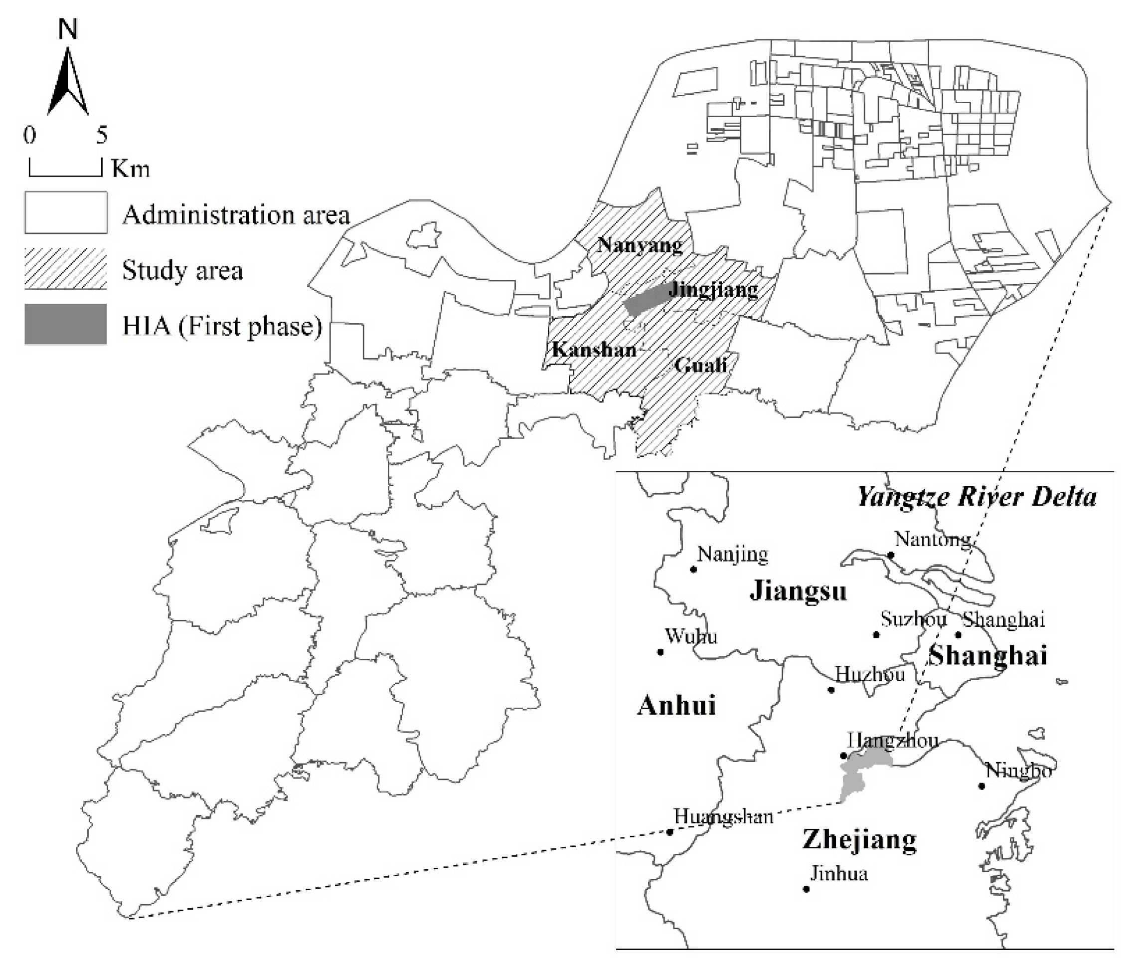
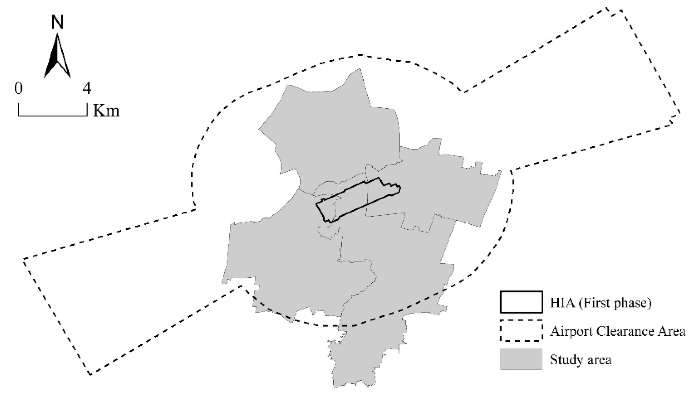
2.1. Airport Overview and Study Area

HIA, one of the main international airports in the Yangtze River Delta in China, currently covers an area of 10 km2 in Xiaoshan District and is located 25 km away from the main center of Hangzhou in Zhejiang Province (Figure 1). The construction of HIA can be divided into three stages, as designed at the initial stage: the first phase of construction started in July 1997 and came into service in December 2000; the second phase began in November 2007, with operations beginning in December 2012; and the third phase is scheduled to be launched in 2035. Before airport construction, the study area was dominated by cultivated land, and the life style was mainly characterized by farming. However, after construction, this area developed into a transportation hub in Eastern China, and by the end of 2016 the annual passenger throughput reached 30 million and HIA was ranked as one of the world’s busiest airports (http://mt.sohu.com/20161218/n476225730.shtml). This tremendous change after construction qualifies HIA as a good case for the study of an airport’s effect on LUCC.
To analyze the effect of HIA on LUCC or the ecological environment, four adjacent towns, Guali, Jingjiang, Nanyang, and Kanshan, were selected as the study area. These towns both intersect with the range of HIA and constitute the main part of the Hangzhou Airport Economic Zone surrounding HIA (http://kg.xsnet.cn/html/ghjs/yqgh/) (Figure 1). Thus, we mainly focus on the effects of the airport on LUCC in the close vicinity of the airport. In addition, we focus on only the first-phase construction of HIA from 1997 to 2000, because if considering the second phase, then the effect of the airport on LUCC will be a mix between those two periods. Notably, the analysis of HIA in the following represents only the first phase, and regarding the research area and time horizon, the effect of airport construction on LUCC discussed in this study focuses on merely the small scale and the short term.

2.2. Data Sources

In line with the start and end time of the first phase of construction from 1997 to 2000, Landsat (https://landsat.usgs.gov/) Thematic Mappers (TM) in 1996 and 2001 were collected. Between them, 1996 represents the land use status before airport construction, while 2001 depicts the land use pattern after airport construction. In addition, TM images in 1986 and 1991 were chosen for the simulation in 1996 and images in 1991 and 1996 were selected for the simulation in 2001. The simulated land use pattern in 1996 was used to compare with the interpretation in 1996 to evaluate the accuracy of the simulation method adopted in this study. The comparison of the simulated and interpreted land use pattern in 2001 was treated as the effect of airport construction on LUCC. All TM images were taken with the path/row: 119/39 for Landsat 3 and Landsat 5. The exact times the images were taken were 8 July 1986, 15 August 1991, 23 August 1996, and 4 October 2001 (http://www.gscloud.cn). They have a 30-m ground resolution (except for the thermal IR band (band 6), which has a 120-m resolution), and all cloud cover is under 5%.

3. Methodology

3.1. Land Use and Land Cover Interpretation

The land use and land cover patterns for 1986, 1991, 1996, and 2001 were derived from TM images by interpretation. Many interpretation techniques have been developed, but no single approach or algorithm is a panacea for all cases [29]. The implementation of the interpretation method depends on the data set itself [30]. Given that the image resolution is low and the number of bands is adequate, supervised classification was the main method applied to classify the land use type from TM images [31,32]. First, the land use classification system proposed by Liu [33], who classified land use types into six primary land types in China, i.e., cultivated land, forest, grassland, urban and rural constructed land, water, and unused land [34,35], was adopted and modified according to the natural characteristics of the study area. Specifically, (1) unused land was abandoned because in this case, there is no unexploited land; (2) road land was proposed as a new type for the linkage or interactive analysis with the constructed land in the following context; and (3) urban and rural constructed land was redefined as constructed land excluding road land. Therefore, the research area was interpreted and classified into six categories: cultivated land, forest, grassland, road, constructed land, and water (Table 1). Then, the training site areas for each class were selected in terms of polygonal training data, and 43 training site areas were determined for all classes through human–computer interaction. Based on the training site areas, the maximum likelihood algorithm was executed to classify the whole TM image into six predefined categories. In addition, to separate the road and constructed land precisely and improve the accuracy of land use mapping, visual interpretation was integrated with the supervised classification result since, in visual interpretation, the human mind is excellent at interpreting spatial attributes and able to identify obscure or subtle features [36] and it is easy to figure out the road due to its linear attribute under naked eyes.
Before concluding with the interpreted land use classes, an accuracy assessment was conducted by randomly choosing 300 ground-based points to represent different land use classes for four classified land use maps. The accuracies of the use and the producer were 90.1% and 82.7% in 1986, 89.6% and 84.5% in 1991, 92.4% and 82.3% in 1996, and 93.7% and 83.5% in 2001, respectively. The overall accuracy reached a high level of 80.7%, 81.3%, 80.6%, and 82.1% in 1986, 1991, 1996, and 2001, respectively. Thus, the accuracy of the interpretation results is suitable for further analysis and discussion [32].

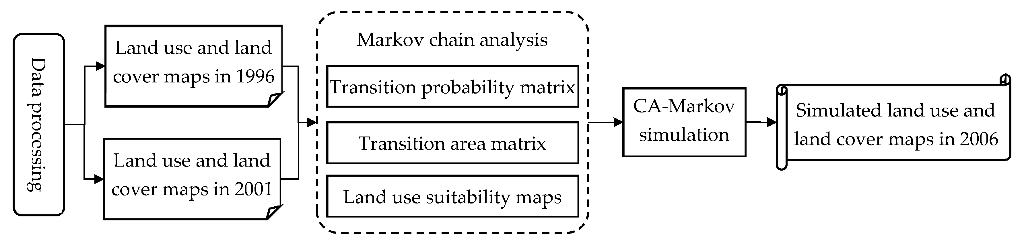
3.2. Counterfactual Analysis and the Cellular Automata (CA)–Markov Model

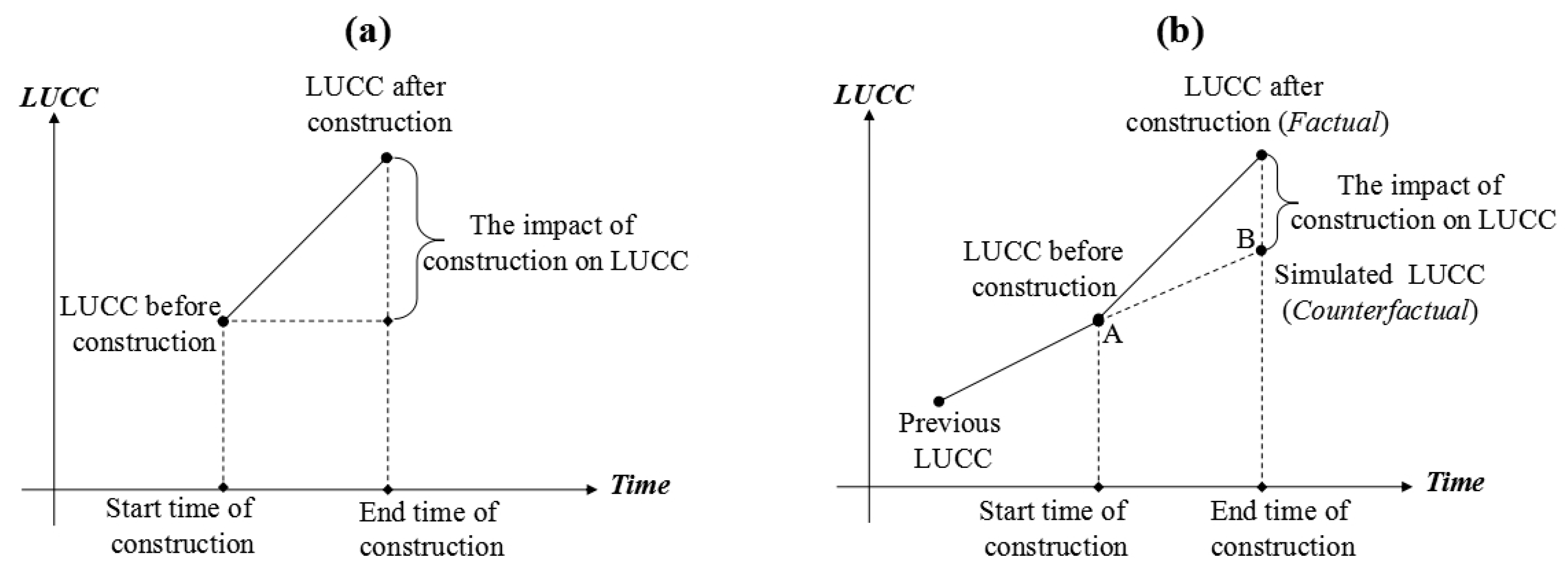
3.2.1. Counterfactual Analysis

In light of the research objective, we follow the idea of counterfactual analysis, which tries to evaluate the effect of a policy on the economy or society through the comparison of fact and counterfact [37]. The fact refers to the status after the implementation of the policy over a period of time, while the counterfact represents the status without the execution of the policy during the same time. The difference between fact and counterfact is the “treatment effect”, which depicts the influence of the policy [38,39,40]. Similarly, the land use pattern after the construction of HIA is the fact, and if we can create a counterfact of the land use pattern that hypothesizes without the intervention of airport construction, then the variance of fact and counterfact is the effect of airport construction on LUCC. Therefore, the key point here is to determine a counterfactual land use pattern that never existed. The simulation of the land use change is a possible way.
In Figure 2, the picture on the left (panel a) is the traditional way of evaluating the impact of infrastructure on LUCC through before and after comparison. The picture on the right (panel b) is the counterfactual method (or simulation method) of evaluating the influence of infrastructure on LUCC by comparing the land use pattern after construction (fact) and the simulated land use pattern (counterfact). The intervention of airport construction disturbed the inherent tendency of the land use change, having a violent impact on the study area. Without the construction of HIA, we assume that the land use pattern would change following the inherent trend of the past. The land use pattern during the same construction period can then be simulated according to the historical spatial-temporal land use change by a cellular automata (CA)–Markov model. Note that the dotted line between A and B in panel b does not necessarily mean a linear change; it just represents that the land use will change following the tendency of the past.

3.2.2. CA–Markov Model

Some studies suggest that land use change is a process with typical Markov properties [41], and a Markov model based on these properties can be used to predict the next status by taking into account the past states [42]. Due to its ability to quantify the conversion among various classes of land use as well as their transfer rate [43], a Markov model can predict the land use change at time t + 1 based on the quantity structure of land use at time t through a conversion probabilities matrix derived from the previous land use conversions among each land use class [44]. This method is appropriate for quantity predictions of land use change [45], but it has a limited capacity in spatial terms because it ignores the change in spatial patterns [46]. The CA is a dynamic and synchronous model where the cell’s state and its neighborhood situation at the current point in time decide its state at the next moment. It has a strong capability to handle the spatiotemporal dynamic evolution within complex spatial distribution systems [47]. Through the local interaction of land units that are based on the transition rule that the state of a land unit at the next stage is determined by its state at the present time as well as its neighborhood situation, a CA model can model the dynamics of land use change from the bottom up over several iterations. However, it is difficult to achieve a “top-down” macro land use pattern and to accurately determine the quantity change in land use [48].
Therefore, by combining the two models as a CA–Markov model that can compensate for the shortcomings of each model and integrate their respective advantages [49], we are able to predict the spatial distribution and the quantity structure of land use change and to realize the local and global dynamic simulation [50,51]. According to the historical land use data (e.g., from 1991 to 1996), the quantities and proportions of conversion among each land use type can be extracted with Markov chain analysis. This conversion information includes the transition probabilities among various classes of land use change as well as the transition area among them, which were treated as a transition probability matrix and a transition area matrix, respectively. The transition probability matrix serves as the transition rule under the CA model, and the transition area matrix is the guideline for the quantitative transformation for simulating land use change (e.g., from 1996 to 2001). In addition, the data of slope extracted from the digital evaluation model (DEM) maps with 30-m resolution and the data of distance to roads, rivers, and urban areas derived from interpreted land use and land cover maps were combined to produce the land use suitability maps. Besides, the number of iterations was set as 5, which is consistent with the time interval in the research period, and the standard 5 × 5 contiguity filter was used as the neighborhood definition under CA. The simulation process of land use change was carried out using IDRISI software (https://clarklabs.org/) and is listed in Figure 3.

3.2.3. Simulation Accuracy Verification

Before discussing the simulation method of evaluation, it is necessary to validate the effectiveness of the model through accuracy verification for further research. To that end, two ways of accuracy verification were applied: the one-to-one cell basis and the overall comparison method [52]. The one-to-one cell basis focuses on calculating the similarity of the simulation and the interpretation through a point-by-point comparison, and the Kappa coefficient is a suitable index to reflect this similarity [53]. The overall comparison method emphasizes the global similarity of the pattern, and the total amount of land use types was compared in this study.

4. Results

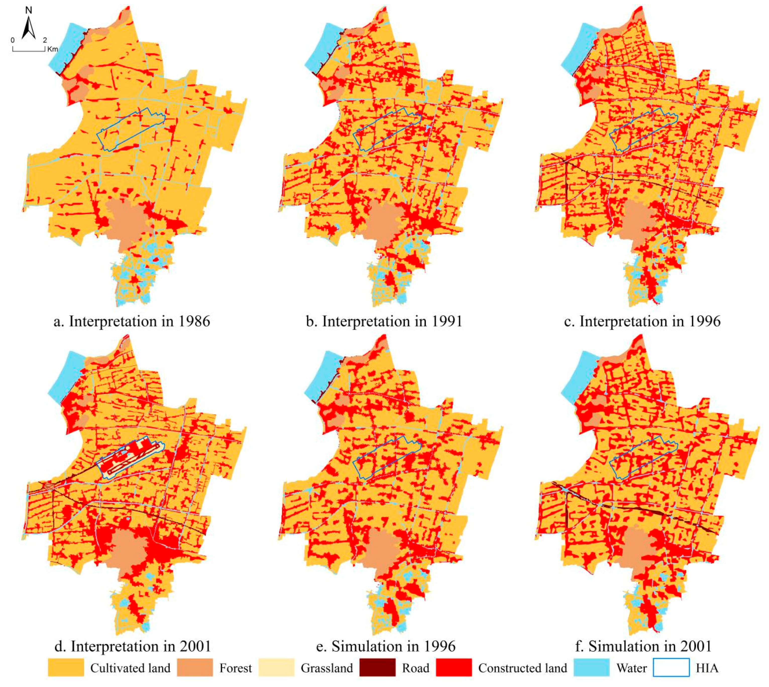
4.1. Interpreted and Simulated Land Use and Land Cover Maps

Based on the above methods, the interpreted or simulated land use pattern of different years can be achieved (Figure 4). Figure 4a–d were derived from TM images and reflect the empirical land use pattern in each year. Figure 4e,f depict the simulated land use pattern in 1996 and 2001. Between them, the empirical land use pattern simulation is based on the interpretation of 1986 and 1991 and is used to validate the accuracy of the model, and the simulated land use pattern is grounded in the interpretation of 1991 and 1996 and is used to evaluate the effect of airport construction on LUCC.
The interpretation and simulation of the land use pattern in 1996 were compared, and the variance between them can reflect the accuracy of the CA–Markov model adopted in this study to a large extent. According to the simulation and interpretation in 1996, the value of the Kappa coefficient between them is 0.7873 at the 1% level of significance, which means that the accuracy of the simulation is acceptable. Furthermore, Table 2 lists the quantity variance of the land use types under simulation and interpretation and shows that, from the perspective of the change ratio, except for roads, the difference between them is very small compared with the base. Therefore, the CA–Markov model is considered suitable in this study.

4.2. Comparison before and after HIA Construction (Traditional Method of Evaluation)

The spatial pattern of land use before and after the construction of HIA has changed significantly as compared in Figure 4c,d. After airport construction, the newly increased constructed land was mainly placed within the range of HIA and was blocked at the southwest region of the study area, which is approximately 3.5 km away from HIA and is located in surrounding forest land (it is a mountain with forest and is surrounded by newly residential land as shown in a high-resolution remote sensing image in Google Earth (https://earth.google.com/web/)). Meanwhile, the decreased cultivated land is also concentrated in these areas, while the new grassland is concentrated in the range of HIA as ancillary land for airport construction, and the new road land is mainly composed of airport roads within the airport and the expressway connecting the main center. In the range of HIA, the land is dominated by planted grassland, constructed land, and roads after the intervention of HIA construction.
In terms of the quantity change in land use (Table 3), after airport construction, the cultivated land, forest, and water in the study area decreased by 465.21, 39.51, and 45.05 ha from 1996 to 2001, respectively. The reduction in those land use types was mainly developed for transformation, thus illustrated as the increasing grassland (from 0 ha to 201.70 ha), constructed land (from 3568.01 ha to 3733.47 ha), and road (from 100.22 ha to 282.83 ha). However, in 2001, cultivated land remained the main type of land use in the study area (at 56.17%) followed by constructed land, water, forest, and road.
The details of conversion among the various land use types can be further found in Table 3. For instance, approximately 1535.65 ha of cultivated land were converted and compose the major part of the newly constructed land during airport construction. This finding means that the major loss of cultivated land occurred mainly due to the massive occupation of newly constructed land while approximately 1215.42 ha of constructed land were transferred to cultivated land at the same time, which means that a massive amount of constructed land has been reclaimed as cultivated land. The main reason is that airport construction caused land expropriation, with the result that some villages and towns were reclaimed as cultivated land. The transfer between cultivated land and constructed land is the major feature of the land use change during this period.
The LUCC shown above reflects both the spillover and direct effects of airport construction on LUCC without separating the direct occupation of airport construction, which is too large to be ignored. Admittedly, the land use change within the study area cannot exactly and completely represent the spillover effect of airport construction on LUCC because it is hard to evaluate/incorporate the influence of airport construction on the wider area. However, with regard to the scope of the impact of airport construction, which itself is an unfixed problem [54], the presented analysis clearly shows the spillover effect of HIA. The quantity changes in land use within the range of HIA are illustrated in Table 4. During the research period, cultivated land just disappeared, while grassland increased 201.71 ha from scratch, and constructed land and road increased 28.96 and 85.30 ha, respectively. Therefore, the direct effect of HIA on LUCC resulted in the conversion of natural land use (mainly composed of cultivated land before airport construction) to converted land use (dominated by planted grassland, constructed land, and road after airport construction).
In brief, from the traditional perspective, the effect of HIA construction on LUCC results in a massive decrease in cultivated land and a large increase in converted land, which is mainly composed of constructed land, road, and grassland. The land use change within the vicinity of the airport is particularly extensive, and the intervention of the airport also stimulated the agglomerative development of constructed land, which means that most of the new constructed land was in the range of HIA.

4.3. Comparison between Interpretation and Simulation in 2001 (Simulation Method of Evaluation)

We compared the quantity variance of land use types between the simulation and interpretation in 2001 and the results listed in Table 5. From the percentage perspective, the difference between the simulation and interpretation is not notable. Almost all of the percentage variance is under 3% except constructed land. The reason for this finding may be that the total study area is large enough to alleviate the variance of airport construction on LUCC. However, if we focus on the area variance, the comparison results are very interesting and meaningful. The simulated data of cultivated land, forest, and road are less than the reality, while the data for constructed land and water are larger than the reality. This result implies that if the land use change had followed the previous tendency and no intervention of airport construction had taken place in the study area, then cultivated land would have decreased by more than 82.07 ha, constructed land would have increased by more than 408.49 ha, less than 136.42 ha of road would have been developed, and extraordinarily, grassland may never have emerged compared with the scale of it in reality in 2001.
In addition to the variation in quantity, the spatial distribution of land use types also differs (Figure 4). Compared to the spatial distribution pattern of land use after airport construction (Figure 4d,f), which has been discussed above, the simulated land use pattern varies. As shown in Figure 4f, cultivated land is still the dominating land use type in the range of HIA, and no grassland exists within it; in the whole study area, there is no obvious agglomerative development of constructed land compared to the reality, and the newly increased constructed land mainly sprawls out through building on the original location of the constructed land, as shown in Figure 4b,c, while cultivated land shrank and was gradually nibbled away by the original constructed land. These results imply that the construction of HIA resulted in the agglomerative development of constructed land and a concentrated decrease in cultivated land.
In short, from the counterfactual perspective, the intervention of HIA construction has decelerated the decrease in cultivated land and limited the increase in constructed land dramatically.

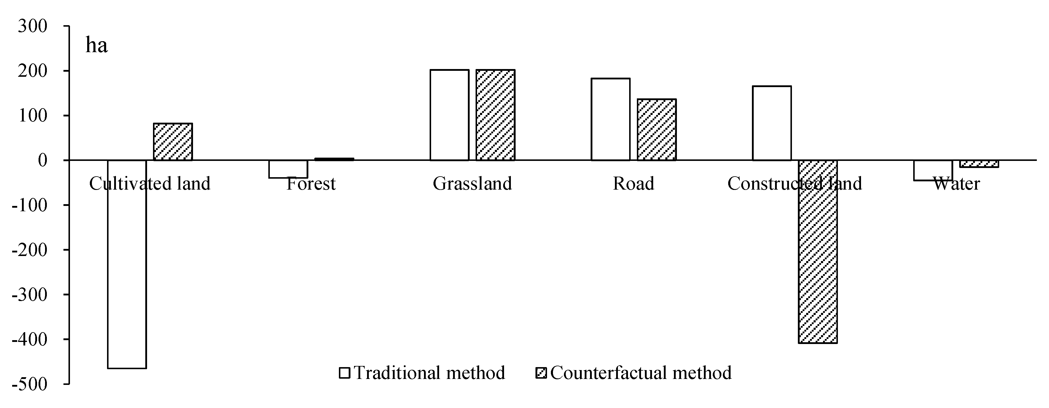
4.4. Variance of the Two Different Methods of Evaluation

The opposite results of the two different methods of evaluating the direction and extent of the airport’s impact on LUCC are illustrated in Figure 5. This figure shows that (1) there is an inconsistency in the effect direction among cultivated land, forest, and constructed land, with the traditional method of evaluation showing that cultivated land and forest have decreased and constructed land has increased but the counterfactual method illustrating that more cultivated land and forest seem to be preserved and newly constructed land has increased less. This figure also shows that (2) there is an inconsistency in the extent of the effect between road and water, in which road has increased and water has decreased, regardless of whether HIA had been constructed or not, but less road seems to be developed and less water seems to be reduced under the counterfactual method.

5. Discussion

In the following, we discuss possible reasons for the land use change after airport construction from the perspective of previous research. Then, we focus on explaining why airport construction could decelerate the reduction in cultivated land and limit the increase in constructed land. In addition, we also reveal some flaws of the simulation model adopted in this study and point out possible directions for future research.

5.1. Explanation of the Land Use Change after Airport Construction

Indeed, the construction of an airport, such as HIA itself, has to occupy a certain amount of land for normal operation; this land includes the land for the terminal, heavy industries, businesses, offices, or even residential buildings due to the growth of laborers working in the airport [25]. Additionally, covering land for transportation, such as the highway for connecting to the outside and the airport runway for plane movements, is a prerequisite for airport operation [55]. Containing the ancillary land mainly involves the planted grassland within and adjacent to air operations areas or other critical locations, and it is also necessary due to specific safety requirements [55]; for example, 39% to 50% of airport properties in the contiguous United States are covered by planted grassland [56]. In addition, the scope of the influence of airport construction is far from being limited to its range [57]. Airport construction can also bring or enhance the advantage of transportation convenience. The economic or traffic location of land in the airport’s surrounding area will therefore be reconstructed and become attractive to developers or the government for pursuing higher economic output, and hence, it might be gradually be converted into factories or other construction uses, even the construction of an airport city [58]. The ultimate result will reflect land use change in the form of an increase in constructed land increasing and a decrease in cultivated land. In brief, the land use change before and after airport construction represents the actual transformation among land use classes; it just shows us an objective change result, but it is too premature to conclude that they are completely stimulated by the intervention of airport construction.

5.2. Explanations for Why Airport Construction Decelerates the Decrease in Cultivated Land and the Increase in Constructed Land

5.2.1. Limitation of the Airport Clearance Area

The setting of the airport clearance area limits additional construction activities. The clearway is extended on both sides by a lateral surface, the slope on the horizontal of which (14.3% or 20%) depends on the type of aircraft being dealt with. The objective of the clearway is to ensure that there are no obstacles above the runway in case of short take-offs or interrupted landings [59]. To protect the movements of aircraft on and above the runway during landings and take-offs, the boundary of the airport clearance area is set to define the maximum height tolerated on and around airfields. According to the Civil Aviation Law of China, it is forbidden to engage in some activities within the scope of a civil airport and the airport clearance area; these activities include the construction of buildings or facilities that affect the electromagnetic environment of the airport, the construction of buildings or facilities that may affect flight safety, or construction that does not meet building requirements [60]. These prohibitive regulations will limit the height of the surrounding buildings and the use of building materials in the spatial distance to the airport to some extent (Figure 6), which may affect land use development.

5.2.2. Impacts of Aviation Noise or Pollution

There are negative effects of aviation noise and pollution on residential or other related constructions. Aviation noise and pollution have the greatest impact on the environment [61], which maintains a close relationship with normal living or working. According to some previous studies, aviation noise exerts a strong, independent, and negative effect on residential values [62]. Residential property values will fall 0.50% and 0.60% for every decibel increase in aviation noise [63]; in particular, the effect of aviation noise is higher for vacant land than for detached housing [64]. Some also suggest that the closer one is to the airport area, the noisier it will be and, in turn, the lower the value of the land will be [65]. Therefore, if the attractiveness for residential development or suitability for living decreases, less residential land will be developed near the airport area. This phenomenon may also explain why the newly constructed land (mainly composed of residential land) was blocked at the south region of the study area and kept 3.5 km away from HIA after airport construction in the previous context. In addition, our field survey in three villages surrounding HIA in 2015 showed that most of the farmers complain about the noise pollution, and therefore, during the second phase of airport construction and land expropriation, the local government had to pay additional money as compensation for the aviation noise. Furthermore, a smaller residential area usually means that businesses or social activities will also be limited due to the lower population.

5.2.3. Restriction of the Land Use and Land Management System in China

The land use and land management system in China, mainly the cultivated land requisition-compensation balance (gengdi zhanbu pingheng, CLRCQ) policy and the land expropriation (tudi zhengshou, LE) regime, also plays a key role. The former was proposed in 1997 and aims to keep the “dynamic balance” (i.e., no net loss) of cultivated land at the county level (e.g., the Xiaoshan government). The main essence of the CLRCQ policy is that regardless of how much cultivated land is occupied by construction, it is obligatory to compensate for this land with the corresponding amount and quality of cultivated land from other areas within the county [66]. Under this policy context and given the massive reduction in cultivated land in the range of airport construction mentioned above, this policy means that the pressure to conserve a certain amount of cultivated land for the local government will be more intense at least in the short term. Therefore, the local government will be more cautious in allowing the occupation of cultivated land outside of the airport area.
According to the LE regime, the local government should first collect land from farmers or residents, with the expense of compensation for them, and then lease the land for airport construction. In an episode before land leasing, to win the site selection for HIA in Xiaoshan District during the earlier site selection stage in 1992, the local government made a promise to the provincial government that it would provide 334 ha of land for airport construction free [67]; however, the local government had to compensate the farmers for the land that they lost by itself. Hence, the local government actually took out a considerable amount of capital to attract HIA located in Xiaoshan District, and based on the contract signed with the farmers or village collectives, the total cost of land expropriation was approximately 108.25 million RMB at least at that time, even without considering the input of land leveling for airport construction and other related capital investments, such as the cost of resettlement for the farmers who lost their land (according to the land expropriation contract, the standard of land expropriation for cultivated land is 15 thousand yuan per mu (equal to 666.67 square meters) and 7.5 thousand yuan per mu for the non-cultivated land, and the compensation for a house, in which the occupied land is a kind of constructed land, is unclear with little information. However, according to the actual situation of land expropriation in China, it is much higher than other types of land compensation). However, the year’s fiscal revenue of the Xiaoshan government was 420.18 million RMB at that time (the fiscal data are from the Statistical Yearbook of Xiaoshan in 1998), which means that 25.76% of government revenue was invested in the land acquisition for the airport project alone. Given that the local government invested massive capital resources in the airport project, less capital will be available for other kinds of development and other land expropriation in the short term. Several official documents, as submitted to the provincial government, also recorded that the local government frequently complained about the pressure of capital (the complaints have frequently occurred in some special reports about the land expropriation and construction of HIA written by the Xiaoshan government and submitted to the provincial government). Therefore, the increase in constructed land and the decrease in cultivated land may also be affected to a large extent by the limitation of the financial conditions of the local government.

5.2.4. The Shadow of the Future

Apart from the above explanations, the uncertainty and certainty of HIA constructions in the future may also have had an influence or shadow on the land use change. The HIA started to operate at the end of 2000, and there remained some uncertainties during the period 1996–2001, such as whether the construction or operation of HIA would be successful or fail and whether or not the operation of the airport would stimulate local socioeconomic development, to say nothing of imaging whether it would grow to become a transportation hub in Eastern China at an earlier stage. Those kinds of uncertainties may have limited the activities of land development in the surrounding area of HIA.
However, considering the strong support of the government, such as the relatively easy method of land expropriation and the adjustment of land use planning for airport construction, which were almost dominated by the government in China, the successful construction and operation of HIA in the future were a high-probability event and could be treated as a future certainty; however, successful construction and operation also would have affected the LUCC in turn at that time. For example, during airport site selection, to promote the land expropriation process before airport construction and to compensate less money to the farmers and residents who lost their land, the local government enacted some kinds of administrative documents to forbid the preemptive construction of farmers or residents in the range of HIA and the surrounding areas because the compensation for constructed land including residences is higher. For example, in September 1993, the circular on the necessary control within the site of the new Hangzhou Civil Airport was announced by the Xiaoshan government; according to it, the control area reached 47 thousand mu, including the whole airport area and most of the study area, and within those areas, new or expanding construction activities were forbidden until the land expropriation for airport construction was finished. The execution of those compulsory regulations could have inevitably decelerated the increase in constructed land in the following years to a large extent.
Furthermore, according to the land use planning and the master plan that was mostly conducted by the local government, the surrounding area of HIA was planned to be a comprehensive service zone, an aviation industrial zone, and an aviation logistics zone in the future (Source: http://kg.xsnet.cn/). However, most of the land was still collectively owned by the collective economic organization or farmers, meaning that the local government also needed to collect land from farmers with the expense of compensation for future development. To avoid higher compensation for local inhabitants in the future, the government might also have adopted some kinds of measures to limit new construction activities for the same reason that the compensation for constructed land was higher than that for other types of land, especially considering the actual compensation for the demolition of farmers’ or residents’ houses in China. Thus, regarding the planned development in the future, land use decision-making might also have affected and resulted in decelerating the increase in constructed land and the decrease in cultivated land.

5.3. Limitations and Possible Improvements in the Future

5.3.1. Other Ignored Factors

Notably, the change in land use patterns may not exclusively have been stimulated by the construction of HIA. There are still many other factors, i.e., population and economic growth as well as other land use policies or the government’s land use decisions, which have not been discussed in this research. For instance, the establishment of Hangzhou Aviation City based on HIA may have attracted more companies or population to settle in the surrounding area, and the land demand for construction would have increased correspondingly. Again, to secure food resources in the late 1990s, the central government executed the “toughest” land regulatory regime trying to control the conversion of cultivated land through a number of quotas [68]. It remains unclear whether those regimes or quotas also protected cultivated land or eliminated the impulse of construction land expansion; this point is still ambiguous.

5.3.2. Exclusive Focus on Short-Term and Small-Scale Effects

As mentioned above, this study focuses only on the land use change within four intersecting towns surrounding the airport from 1996 to 2001, which means that, in a sense, the influence of airport construction on LUCC merely concerns small-scale and short-term effects. Therefore, the results of this study should not be extrapolated to a larger scale and longer term, and whether the large-scale and long-term effect of airport construction on LUCC has the same outcome or not remains unclear. Conducting more extensive research is needed in the next step. In addition, the lack of a case comparison may also limit the application of the results. Thus, more broadly similar research on other airport cases should to be conducted in the future before we generalize the findings of this research.

5.3.3. Limitation of the CA–Markov Model

No model can simulate all aspects of reality 100% correctly, even if the validation of the CA–Markov model made it suitable for this research. Thus, one important limitation still exists. The basic assumption of a CA–Markov model is that the transition probability of land use types extracted from previous land use change is constant [69]. However, the land use change was affected by many factors [70], and the synthesis of those factors resulted in the variance of transition probabilities among land use types. Specifically, the factors are also dynamic and will change over time; thus, the transition probability will be inconstant. If cultivated land keeps decreasing and constructed land keeps increasing, as shown in Figure 4a–c, the study area will ultimately be dominated by constructed land and will lack any cultivated land until one day, which will not happen. There are two possible ways to alleviate this shortcoming. One way is to shorten the time interval of the simulation, as LUCC is approximately constant in the short term [71]. Another way is to identify the main factors that affect land use change in different periods and take them into account correspondingly by combining a CA–Markov model with a multi-criteria evaluation.

6. Conclusions

Infrastructure construction is one of the main tasks for developing and developed countries in the long run, and it is essential to evaluate the effect of infrastructure on the natural system, particularly regarding the effect on land resources, which are the main carrier for infrastructure, to maintain environmental sustainability. Herein, through a case study of Hangzhou International Airport (first phase) in the Yangtze River Delta in China, the land use change surrounding the airport was detected by remote sensing, and the short-term effect of airport construction on LUCC at a small scale was evaluated through simulation.
According to the actual land use pattern before and after airport construction, cultivated land has decreased dramatically, and constructed land and road have clearly increased, accompanying airport construction in the study area, especially in the range of the airport. These results illustrate that airport construction did have an extensive influence on LUCC; however, it is too far a step to conclude that the increase in constructed land and the decrease in cultivated land were stimulated by airport construction because the comparison of before and after has just ignored the fact that even without the intervention of HIA, the land use pattern also would have changed dynamically.
In contrast, according to the counterfactual simulation result, airport construction has decelerated the decrease in cultivated land and the increase in constructed land at least in the short term and at a small scale. Possible reasons for this finding are that the airport construction not only brought transport convenience and economic growth for the local region but also produced some affiliated outputs, such as the boundary setting of the airport clearance area and the corresponding aviation noise or pollution, which introduced some restrictions for general construction activities and, in particular, affected normal residential living around the airport. Moreover, the construction of HIA had an obvious attribute of administrative intervention, such as the local government’s promise to the provincial government without the agreement of the people or the issued rules of restrictions on construction to reduce future compensation payments. Combined with the unique characteristics of the land use and land management system in China, these factors may be composed together to establish an invisible power to limit the newly constructed land and to conserve the cultivated land to some extent. Besides, given the effects of airport construction on LUCC we found, it is meaningful to further simulate the LUCC under the background of infrastructure expansion in follow-up researches, as it may help to provide hints for land use planning or decision-making in China or other countries.
From this study, a good lesson can be drawn for further similar research on land use change. We contend that by following the idea of counterfactual analysis, the simulation method is suitable and takes a further step in evaluating the effect of infrastructure construction on LUCC as compared with the before and after comparison method, which may draw biased conclusions. Beyond that point, observing the results of land use change, we argue that the key actor’s activities and the underlying fundamental institutions should not be ignored. Particularly in China, with its strong characteristic of administrative intervention in land use or land management, we support the need for a deep analysis of the institutional and the key land use actors embedded in the phenomenon of land use change. Their influence should be taken into account when discussing the land use change in China and in other similar countries.

Author Contributions

C.X. and R.T. conceived and designed the study, carried out data analysis and wrote the draft paper; V.B. led the manuscript revision and modification, and helped improve other parts. All authors read and approved this version.

Acknowledgments

This research has received financial support from the Natural Science Foundation of China through project No. 71573231, the Social Science Foundation of China through project No. 16ZDA020, No. 14AZD028, No. 13AZD012 and No. 14ZDA039. The authors would like to thank the funding organizations for the grants. We would like to thank Lu Yu and Klaus Eisenack for their helpful comments on earlier drafts. The valuable reports from four anonymous reviewers are also much appreciated.

Conflicts of Interest

The authors declare no conflict of interest.

References

  1. National Development and Reform Commission, Ministry of Foreign Affairs, Ministry of Commerce. To Promote the Construction of the Silk Road Economic zone and the 21st Century Maritime Silk Road Vision and Action. Available online: http://www.mofcom.gov.cn/article/resume/n/201504/20150400929655.shtml (accessed on 2 April 2018). (In Chinese)
  2. Kumatani, K.; Takahashi, E.; Kato, T. Current and future infrastructure networks aimed at resolving issues related to the changing and diversifying activities in society. Fujitsu Sci. Tech. J. 2013, 49, 271–279. [Google Scholar]
  3. Hensher, D.A.; Truong, T.P.; Mulley, C.; Ellison, R. Assessing the wider economy impacts of transport infrastructure investment with an illustrative application to the North-West Rail Link project in Sydney, Australia. J. Transp. Geogr. 2012, 24, 292–305. [Google Scholar] [CrossRef]
  4. Beyzatlar, M.A.; Tepeli, M.Y.I.K. Infrastructure, economic growth and population density in Turkey. Int. J. Econ. Sci. Appl. Res. 2011, 4, 39–57. [Google Scholar]
  5. Bougheas, S.; Demetriades, P.O.; Mamuneas, T.P. Infrastructure, specialization, and economic growth. J. Econ. Rev. Can. D Econ. 2000, 33, 506–522. [Google Scholar] [CrossRef] [Green Version]
  6. Easterly, W.; Rebelo, S. Fiscal policy and economic growth. J. Monet. Econ. 1993, 32, 417–458. [Google Scholar] [CrossRef] [Green Version]
  7. Sanchez Robles, B. Infrastructure investment and growth: Some empirical evidence. Contemp. Econ. Policy 1998, 16, 98–108. [Google Scholar] [CrossRef]
  8. Canning, D.; Pedroni, P. Infrastructure, long-run economic growth and causality tests for cointegrated panels. Manch. Sch. 2008, 76, 504–527. [Google Scholar] [CrossRef]
  9. Demetriades, P.O.; Mamuneas, T.P. Intertemporal output and employment effects of public infrastructure capital: Evidence from 12 OECD economies. Econ. J. 2000, 110, 687–712. [Google Scholar] [CrossRef]
  10. Calderón, C.; Moral Benito, E.; Servén, L. Is infrastructure capital productive? A dynamic heterogeneous approach. J. Appl. Econom. 2015, 30, 177–198. [Google Scholar] [CrossRef]
  11. Calderón, C.; Servén, L. The Effects of Infrastructure Development on Growth and Income Distribution; World Bank Publications: Washington, DC, USA, 2004. [Google Scholar]
  12. Venables, A.J. Evaluating urban transport improvements: Cost–benefit analysis in the presence of agglomeration and income taxation. J. Transp. Econ. Policy (JTEP) 2007, 41, 173–188. [Google Scholar]
  13. Wu, J.; Huang, J.; Han, X.; Xie, Z.; Gao, X. Three-Gorges Dam—Experiment in habitat fragmentation? Science 2003, 300, 1239–1240. [Google Scholar] [CrossRef] [PubMed]
  14. Forman, R.T.T.; Sperling, D.; Bissonette, J.A.; Clevenger, A.P.; Cutshall, C.D.; Dale, V.H.; Fahrig, L.; France, R.; Goldman, C.R.; Heanue, K. Road Ecology: Science & Solutions; Island Press: Washington, DC, USA, 2003. [Google Scholar]
  15. Colchero, F.; Conde, D.A.; Manterola, C.; Chávez, C.; Rivera, A.; Ceballos, G. Jaguars on the move: Modeling movement to mitigate fragmentation from road expansion in the Mayan Forest. Anim. Conserv. 2011, 14, 158–166. [Google Scholar] [CrossRef]
  16. Topalovic, P.; Carter, J.; Topalovic, M.; Krantzberg, G. Light rail transit in Hamilton: Health, environmental and economic impact analysis. Soc. Indic. Res. 2012, 108, 329–350. [Google Scholar] [CrossRef]
  17. Yigitcanlar, T.; Dur, F. Developing a sustainability assessment model: The sustainable infrastructure, land-use, environment and transport model. Sustainability 2010, 2, 321–340. [Google Scholar] [CrossRef] [Green Version]
  18. Forman, R.T.T.; Alexander, L.E. Roads and their major ecological effects. Annu. Rev. Ecol. Syst. 1998, 29, 207–231. [Google Scholar] [CrossRef]
  19. Nemerow, N.L.; Agardy, F.J.; Sullivan, P.; Salvato, J.A. Environmental Engineering: Environmental Health and Safety for Municipal Infrastructure, Land Use and Planning, and Industry; Wiley: Hoboken, NJ, USA, 2009. [Google Scholar]
  20. Lambin, E.F.; Meyfroidt, P. Global land use change, economic globalization, and the looming land scarcity. Proc. Natl. Acad. Sci. USA 2011, 108, 3465–3472. [Google Scholar] [CrossRef] [PubMed] [Green Version]
  21. Giuliano, G. Land Use Impacts of Transportation Investments: Highway and Transit; Guilford Press: New York, NY, USA, 2004. [Google Scholar]
  22. Kasraian, D.; Maat, K.; Stead, D.; van Wee, B. Long-term impacts of transport infrastructure networks on land-use change: An international review of empirical studies. Transp. Rev. 2016, 36, 772–792. [Google Scholar] [CrossRef]
  23. Mojica, L.; Martí-Henneberg, J. Railways and Population Distribution: France, Spain, and Portugal, 1870–2000. J. Interdiscip. Hist. 2011, 42, 15–28. [Google Scholar] [CrossRef]
  24. Zhang, Y.; Yan, J.; Liu, L.; Bai, W.; Zheng, D. Effects of Qinghai-Xizang Highway on land use and landscape pattern change: From Golmud to Tanggulashan pass. Acta Geogr. Sin. 2002, 57, 253–266. (In Chinese) [Google Scholar]
  25. Swangjang, K.; Iamaram, V. Change of land use patterns in the areas close to the airport development area and some implicating factors. Sustainability 2011, 3, 1517–1530. [Google Scholar] [CrossRef]
  26. Ferreira, L.; Stevens, N.J.; Baker, D.C. The New Airport and its Urban Region: Evaluating Transport Linkages. Airport Strategic Planning. In Proceedings of the International Conference on Traffic and Transport Studies, Xi’an, China, 2–5 August 2006; pp. 22–29. [Google Scholar]
  27. Karsner, D. Aviation and airports: The impact on the economic and geographic structure of American cities, 1940s–1980s. J. Urban Hist. 1997, 23, 406–436. [Google Scholar] [CrossRef]
  28. Civil Aviation Administration of China, National Development and Reform Commission, Ministry of Transport. China’s Civil Aviation Development of the Thirteenth Five-Year Plan; Civil Aviation Administration of China, National Development and Reform Commission, Ministry of Transport: Beijing, China, 2016. (In Chinese)
  29. Lu, D.; Mausel, P.; Brondizio, E.; Moran, E. Change detection techniques. Int. J. Remote Sens. 2004, 25, 2365–2407. [Google Scholar] [CrossRef]
  30. Zhang, J.X.; Zhang, Y.H. Remote sensing research issues of the National Land Use Change Program of China. ISPRS J. Photogramm. Remote Sens. 2007, 62, 461–472. [Google Scholar] [CrossRef]
  31. Weng, Q.H. Land use change analysis in the Zhujiang Delta of China using satellite remote sensing, GIS and stochastic modelling. J. Environ. Manag. 2002, 64, 273–284. [Google Scholar] [CrossRef] [Green Version]
  32. Campbell, J.B.; Wynne, R.H. Introduction to Remote Sensing; Guilford Press: New York, NY, USA, 2011. [Google Scholar]
  33. Liu, J. Study on national resources & environment survey and dynamic monitoring using remote sensing. J. Remote Sens. 1997, 1, 225–230. (In Chinese) [Google Scholar]
  34. Liu, J.Y.; Liu, M.L.; Zhuang, D.F.; Zhang, Z.X.; Deng, X.Z. Study on spatial pattern of land-use change in China during 1995–2000. Sci. China Ser. D Earth Sci. 2003, 46, 373–384. (In Chinese) [Google Scholar]
  35. Liu, J.Y.; Kuang, W.H.; Zhang, Z.X.; Xu, X.L.; Qin, Y.W.; Ning, J.; Zhou, W.C.; Zhang, S.W.; Li, R.D.; Yan, C.Z.; et al. Spatiotemporal characteristics, patterns, and causes of land-use changes in China since the late 1980s. J. Geogr. Sci. 2014, 24, 195–210. [Google Scholar] [CrossRef]
  36. Lillesand, T.M. Remote Sensing and Image Interpretation; Wiley: Hoboken, NJ, USA, 1979; pp. 3035–3038. [Google Scholar]
  37. Rubin, D.B. Estimating causal effects of treatments in randomized and nonrandomized studies. J. Educ. Psychol. 1974, 66, 688–701. [Google Scholar] [CrossRef]
  38. Cowan, R.; Foray, D. Evolutionary economics and the counterfactual threat: On the nature and role of counterfactual history as an empirical tool in economics. J. Evol. Econ. 2002, 12, 539–562. [Google Scholar] [CrossRef]
  39. Keohane, R.O. Counterfactuals and causal inference: Methods and principles for social research. Soc. Forces 2009, 88, 466–467. [Google Scholar] [CrossRef]
  40. Abadie, A.; Diamond, A.; Hainmueller, J. Synthetic control methods for comparative case studies: Estimating the effect of California’s Tobacco control program. J. Am. Stat. Assoc. 2010, 105, 493–505. [Google Scholar] [CrossRef]
  41. Muller, M.R.; Middleton, J. A Markov model of land-use change dynamics in the Niagara region, Ontario, Canada. Landsc. Ecol. 1994, 9, 151–157. [Google Scholar]
  42. Brown, D.G.; Pijanowski, B.C.; Duh, J.D. Modeling the relationships between land use and land cover on private lands in the Upper Midwest, USA. J. Environ. Manag. 2000, 59, 247–263. [Google Scholar] [CrossRef] [Green Version]
  43. Sang, L.; Zhang, C.; Yang, J.; Zhu, D.; Yun, W. Simulation of land use spatial pattern of towns and villages based on CA–Markov model. Math. Comput. Model. 2011, 54, 938–943. [Google Scholar] [CrossRef]
  44. Tallis, J.H.; Glenn-Lewin, D.C.; Peet, R.K.; Veblen, T.T. Plant succession: Theory and prediction. J. Ecol. 1993, 81, 830. [Google Scholar] [CrossRef]
  45. Wickramasuriya, R.C.; Bregt, A.K.; van Delden, H.; Hagen-Zanker, A. The dynamics of shifting cultivation captured in an extended Constrained Cellular Automata land use model. Ecol. Model. 2009, 220, 2302–2309. [Google Scholar] [CrossRef]
  46. Tattoni, C.; Ciolli, M.; Ferretti, F. The fate of priority areas for conservation in protected areas: A fine-scale Markov chain approach. Environ. Manag. 2011, 47, 263–278. [Google Scholar] [CrossRef] [PubMed]
  47. Balzter, H.; Braun, P.W.; Kohler, W. Cellular automata models for vegetation dynamics. Ecol. Model. 1998, 107, 113–125. [Google Scholar] [CrossRef] [Green Version]
  48. Yeh, A.G.O.; Li, X. A cellular automata model to simulate development density for urban planning. Environ. Plan. B Plan. Des. 2002, 29, 431–450. [Google Scholar] [CrossRef]
  49. Li, H.; Reynolds, J.F. Modeling effects of spatial pattern, drought, and grazing on rates of rangeland degradation: A combined Markov and cellular automaton approach. Scale Remote Sens. GIS 1997, 211–230. [Google Scholar]
  50. Adhikari, S.; Southworth, J. Simulating forest cover changes of Bannerghatta National Park based on a CA-Markov model: A remote sensing approach. Remote Sens. Basel 2012, 4, 3215–3243. [Google Scholar] [CrossRef]
  51. Subedi, P.; Subedi, K.; Thapa, B. Application of a hybrid cellular automaton-Markov (CA-Markov) model in land-use change prediction: A case study of Saddle Creek Drainage Basin, Florida. Sci. Educ. 2013, 1, 126–132. [Google Scholar] [CrossRef]
  52. Wu, F.L. Calibration of stochastic cellular automata: The application to rural-urban land conversions. Int. J. Geogr. Inf. Sci. 2002, 16, 795–818. [Google Scholar] [CrossRef]
  53. Pontius, R.G.; Cornell, J.D.; Hall, C.A.S. Modeling the spatial pattern of land-use change with GEOMOD2: Application and validation for Costa Rica. Agric. Ecosyst. Environ. 2001, 85, 191–203. [Google Scholar] [CrossRef]
  54. Wijk, M.V.; Brattinga, K.; Bontje, M.A. Exploit or protect airport regions from urbanization? Assessment of land-use restrictions in Amsterdam-Schiphol. Eur. Plan. Stud. 2011, 19, 261–277. [Google Scholar] [CrossRef]
  55. Federal Aviation Administration. Airport Design; Advisory Circular 150/5300-13A; Washington, DC, USA, 2012.
  56. Devault, T.; Kubel, J.; Rhodes, O.; Dolbeer, R. Habitat and bird communities at small airports in the Midwestern USA. In Proceedings of the 13th WDM Conference, Lincoln, NE USA, 2009; University of Nebraska–Lincoln: Lincoln, NE, USA, 2009; Volume 13, pp. 137–145. [Google Scholar]
  57. Kasarda, J.D. Airport cities: The evolution. Airpt. World 2013, 18, 24–27. [Google Scholar]
  58. Reiss, B. Maximising non-aviation revenue for airports: Developing airport cities to maximise real estate and capitalise on land development opportunities. J. Airpt. Manag. 2007, 1, 284–293. [Google Scholar]
  59. Clearance Area of an Airfield. Available online: http://www.planete-tp.com/en/clearance-area-of-an-airfield-a44.html (accessed on 8 January 2017).
  60. Standing Committee of the People Congress. The Civil Aviation Law of People’ Republic of China; Standing Committee of the People Congress: Beijing, China, 1995. (In Chinese)
  61. Cidell, J.L. Scales of Airport Expansion: Globalization, Regionalization, and Local land Use; The University of Minnesota Digital Conservancy: Minneapolis, MN, USA, 2004; p. 313. [Google Scholar]
  62. Collins, A.; Evans, A. Aircraft noise and residential property values: An artificial neural network approach. J. Transp. Econ. Policy 1994, 28, 175–197. [Google Scholar]
  63. Nelson, P. Meta-analysis of airport noise and hedonic-property values-problems and prospects. J. Transp. Econ. Policy 2004, 38, 1–27. [Google Scholar]
  64. Uyeno, D.; Hamilton, S.W.; Biggs, A.J.G. Density of Residential Land Use and the Impact of Airport Noise. J. Transp. Econ. Policy 1991, 27, 3–18. [Google Scholar]
  65. Jud, G.D.; Winkler, D.T. The announcement effect of an airport expansion on housing prices. J. Real Estate Financ. Econ. 2006, 33, 91–103. [Google Scholar] [CrossRef]
  66. Central Committee of the Communist Party the State Council of China. Circular on Further Strengthening Land Administration and Effectively Protecting Cultivated Land; Central Committee of the Communist Party the State Council of China: Beijing, China, 1997. (In Chinese)
  67. Xiaoshan City Government. On the Request of the Hangzhou International Airport Construction Project Address in Xiaoshan; Xiaoshan City Government: Hangzhou, China, 1992. (In Chinese)
  68. Wang, H.; Tao, R.; Wang, L.L.; Su, F.B. Farmland preservation and land development rights trading in Zhejiang, China. Habitat Int. 2010, 34, 454–463. [Google Scholar] [CrossRef]
  69. Kityuttachai, K.; Tripathi, N.K.; Tipdecho, T.; Shrestha, R. CA-Markov analysis of constrained coastal urban growth modeling: Hua Hin Seaside City, Thailand. Sustainability 2013, 5, 1480–1500. [Google Scholar] [CrossRef]
  70. Lambin, E.F.; Turner, B.L.; Geist, H.J.; Agbola, S.B.; Angelsen, A.; Bruce, J.W.; Coomes, O.T.; Dirzo, R.; Fischer, G.; Folke, C.; et al. The causes of land-use and land-cover change: Moving beyond the myths. Glob. Environ. Chang. Hum. Policy Dimens. 2001, 11, 261–269. [Google Scholar] [CrossRef]
  71. Zhou, D.; Lin, Z.; Liu, L. Regional land salinization assessment and simulation through cellular automaton-Markov modeling and spatial pattern analysis. Sci. Total Environ. 2012, 439, 260–274. [Google Scholar] [CrossRef] [PubMed]
Figure 1. Location of the study area.
Sustainability 10 02013 g001
Figure 2. Measuring the impact of infrastructure on regional land use and land cover change (LUCC) through before and after comparison (a) and counterfactual simulation (b).
Sustainability 10 02013 g002
Figure 3. Workflow chart of the cellular automata (CA)–Markov simulation.
Sustainability 10 02013 g003
Figure 4. Land use and land cover maps based on (a) 1986 Thematic Mappers™ images; (b) 1991 TM images; (c) 1996 TM images; (d) 2001 TM images; (e) 1996 CA–Markov model simulation; and (f) 2001 CA–Markov model simulation. HIA, Hangzhou International Airport.
Sustainability 10 02013 g004
Figure 5. Variance in land use change under different methods of effect evaluation. Note: Traditional method means comparing the land use change before and after airport construction, and the counterfactual method means contrasting the interpreted land use data to the simulated land use in the 2001 data (without airport construction).
Sustainability 10 02013 g005
Figure 6. Location of airport clearance area (Source: http://www.hzairport.com/).
Sustainability 10 02013 g006
Table 1. Description of land use/land cover types in the study area.
ClassDescription
Cultivated landRefers to areas cultivated with annual crops, vegetables, or fruit, including newly reclaimed land, paddies, and dry land
ForestRefers to forestry lands, including timber, fuel wood, shelter and economic forests, sparse woodlands, and shrubs
GrasslandRefers to land for growing herbs; it mainly includes planted grassland along with the construction of the airport runway
RoadRefers to infrastructure land for vehicles and pedestrians, mainly including highways and the airport runway
Constructed landRefers to land for construction activities, including urban and rural residences, industry, mining, salt panning, and specially used land (excluding roads)
WaterRefers to land covered by a certain area of water, including rivers, lakes, reservoirs, beaches, canals, and breeding plots
Table 2. Comparison of simulation and interpretation data in 1996 (area in ha).
1996Cultivated LandForestRoadConstructed LandWater
Interpretation7810.09761.15100.223568.01939.46
Simulation7774.39728.8328.203660.83986.68
Area change a−35.70−32.32−72.0292.8247.22
Note: a Area change represents the simulated land use data in 1996 minus the interpretation.
Table 3. Land use change and transfer matrix from 1996 to 2001 (area in ha).
1996 Cultivated LandForestGrasslandRoadConstructed LandWaterTotal
2001
Cultivated land5858.0344.03 136.33148.021535.6588.037810.09
Forest68.19 616.93 0.000.00 69.02 7.01761.15
Grassland0.000.000.000.000.000.000.00
Road15.54 2.46 0.0059.28 8.86 14.08 100.22
Constructed land1215.4257.83 61.9658.522023.58150.70 3568.01
Water187.69 0.38 3.4117.0296.37634.59939.46
Total7344.88721.64 201.70282.833733.47894.4113,178.93
Area change a−465.21−39.51201.70182.61165.46−45.050.00
Note: a Area change represents the land use data in 2001 minus the data in 1996.
Table 4. Land use change in the range of HIA during 1996–2001 (area in ha).
Land Use Type19962001Area Change a
AreaPercentageAreaPercentage
Cultivated land324.2068.79%0.000.00%−324.1
Grassland0.000.00%201.7142.80%201.71
Road0.000.00%85.3018.10%85.30
Constructed land141.0129.92%169.9736.06%28.96
Water6.101.29%14.343.04%8.24
Total of HIA471.31100.00%471.31100.00%0.00
Note: a Similar to that in Table 3.
Table 5. Comparison between the simulated and interpreted land use in 2001 (area in ha).
Land Use TypeSimulation without HIA Construction in 2001Interpretation after HIA Construction in 2001Area Variance aPercentage Variance b
AreaPercentageAreaPercentage
Cultivated land7262.8155.17%7344.88 55.73%82.07 0.56%
Forest717.775.45%721.64 5.48%3.87 0.03%
Grassland0.000.00%201.70 1.53%201.70 1.53%
Road146.411.11%282.83 2.15%136.42 1.04%
Constructed land4142.1631.36%3733.47 28.33%−408.69 −3.03%
Water909.796.91%894.41 6.79%−15.38 −0.12%
Total13,178.93100.00%13,178.93 100.00%0.000.00%
Note: a Area variance represents the interpreted land use data in 2001 minus the simulated land use data; b Percentage variance means the percentage of interpreted land use in 2001 relative to the percentage of land use in the simulation.

