Energy Management for Plug-In Hybrid Electric Vehicle Based on Adaptive Simplified-ECMS

Abstract

When searching for the optimal solution, Equivalent Consumption Minimum Strategy (ECMS) has to calculate and compare the total equivalent fuel rate of huge candidates covered all over the control domain for each time instant. Therefore, this strategy still has a heavy computation burden problem; it is a challenge for ECMS to be implemented online for real-time control. To reduce ECMS’s calculation load, this paper proposes an adaptive Simplified-ECMS-based strategy for a parallel plug-in hybrid electric vehicle (PHEV). A convex piecewise function is applied to fit the total equivalent fuel rate with respect to the motor torque, which is the control variable. Then, the ECMS problem is simplified to calculate and compare only five candidates’ total equivalent fuel rate to determine the optimal torque distribution. Particle swarm optimization (PSO) algorithm is applied to optimize the equivalent factor, and the MAPs of this factor under different driving cycles, driving distances and initial SOC are obtained. Based on this, the adaptive Simplified-ECMS-based strategy is proposed. Simulations were performed, and the results show that the Simplified-ECMS-based strategy can obviously shorten the calculation time compared to ECMS-based strategy, and the adaptive Simplified-ECMS-based strategy can decrease fuel consumption of plug-in hybrid electric vehicle by 16.43% under the testing driving cycle, compared to CD-CS-based strategy. A road test on the prototype vehicle is conducted and the effectiveness of the Simplified-ECMS-based strategy is validated by the test data.

1. Introduction

Plug-in hybrid electric vehicles (PHEVs) assume an essential role in decreasing fuel consumption, pollutant emissions, and carbon footprint [1]. Indeed, the application effect of PHEVs is strongly influenced by many optimization tasks, i.e., charging station’s locating optimization [2,3,4], charging time optimization [4], the PHEV taxi system’s optimization [5], battery size optimization [6], and power optimization during driving. This power optimization is actually the major part of the blended energy management strategy (blend- energy management strategy (EMS)), which is a crucial technology for PHEVs [7]. The main blend-EMSs encompass dynamic programming (DP)-based-EMS [8,9,10,11], derivative-free algorithms (DFA)-based-EMS [12,13,14,15], quadratic programming (QP)-based-EMS [16], pontryagin’s minimum principle (PMP)-based-EMS [17,18], equivalent consumption minimization (ECMS)-based-EMS [19,20,21].

DP-based-EMS is able to compute global optimal solutions for PHEVs. However, it is hard to apply to real-time control for its high computational burden, As a result, DP-based-EMS is widely utilized in offline analysis to benchmark alternative EMSs, inspire RB strategies design, and serve as training data for machine learning algorithms, etc. [12,22]. DFA-based-EMS mainly concern metaheuristic algorithms inspired in nature and DIRECT deterministic method [12], The main DFA-based-EMSs employed by PHEVs are simulated annealing (SA)-based-EMS [13], genetic algorithm (GA)-based-EMS [16], and particle swarm optimization (PSO)-based-EMS [14]. Above EMSs do not require derivative calculations, but these EMSs solve optimization problems with large search space of likely solutions, which causes a high computation load. The aforementioned EMSs have a heavy computation burden problem, some studies explore simplifying technique, instantaneous optimization method or local optimization method to improve computationally efficient, including QP-based-EMS [16], PMP-based-EMS [18], and ECMS-based-EMS [21]. Hu et al. designed QP-based-EMS for a series plug-in hybrid electric bus, and demonstrated its decreasing computational time and the feasibility of real-time control [6]. Nevertheless, this EMS’s limitation lies in its strictly convex terms requirement, which requires that both cost function and inequality constraints are expressed in convex form, and equality constraints are affine [23]. So QP-based-EMS is not suit for PHEVs with complex configuration. PMP-based-EMS has transformed the global optimization problem to an instantaneous Hamiltonian optimization problem, which makes its real-time control possible. However, it is still a challenge for optimizing the Hamiltonian real-time due to the massive computational load required [17]. ECMS-based-EMS was first introduced for a parallel single shaft hybrid powertrains with a constant equivalent factor by Paganelli et al. [24]. ECMS is derived from the pontryagin’s minimum principle. Making some assumptions, simplifications and equations derivation about PMP-based EMS, the local optimization algorithm of ECMS is obtained. These simplifications really improve the algorithm of ECMS’s computationally efficiency. However, ECMS online implementation requires further reduction of the computational time, since candidates of the control variable cover all over the control domain, calculating and comparing the total equivalent fuel of these huge candidates to determine the optimal solution is still a challenge.

Through above analysis, we know that further simplification of optimization algorithm and further reduction of the computational time are very necessary to apply blend-EMSs to PHEVs’ real-time control. ECMS-based-EMS is more likely to be applied to PHEVs with complex configuration’s real-time control than other blend-EMSs. Therefore, we select ECMS algorithm to further simplify it. Firstly, the models of engine’s fuel rate and battery’s consumption rate are approximately fitted by the piecewise function. Then, the total equivalent fuel rate can be expressed by a convex piecewise function. Finally, according to the properties of convex functions, the ECMS problem is simplified to calculate and compare total equivalent fuel rate of only five candidates to identify the optimal torque distribution, instead of calculating and comparing the total equivalent fuel rate of huge candidates, who cover all over the control domain. After gaining the Simplified-ECMS-based strategy, we introduce the particle swarm optimization (PSO) genetic algorithm to optimize the Simplified-ECMS algorithm’s equivalent factor, instead of optimizing this factor by trial and error method. The MAPs of this factor under different driving patterns, driving distances and initial SOC are obtained through off-line optimization based on this genetic algorithm. Finally, the adaptive Simplified-ECMS-based EMS is implemented based on the equivalent factor MAPs.

The original contribution of this paper is related to the following aspects. First, a Simplified-ECMS-based strategy is proposed to simplify ECMS problem and reduce calculation burden. Second, the particle swarm optimization (PSO) genetic algorithm is introduced to optimize the equivalent factor, rather than obtaining the factor by trial and error method. Finally, by integrating the two major contributions mentioned above as well as other works, the adaptive Simplified-ECMS-based EMS is proposed for the EMS of the PHEV.

The outline of this paper is as follows. The structure and parameters of a parallel continuously variable transmission (CVT)-based PHEV powertrain are described in Section 2. The model of the powertrain system is provided in Section 3. Simplified-ECMS-based strategy is proposed in Section 4. The adaptive Simplified-ECMS-based strategy is presented in Section 5. Road test is conducted in Section 6 to validate the effectiveness of the Simplified-ECMS-based strategy. Finally, conclusions are discussed in Section 7.

2. Structure and Parameters of the Powertrain System

This study focused on a single-shaft parallel CVT-based PHEV. Figure 1 shows the powertrain of this vehicle that includes an internal combustion engine (ICE), an integrated starter and generator motor (ISG motor), battery, clutch, a continuously variable transmission (CVT) and final drive (FD). The vehicle runs in different operating modes by controlling the state of the engine and motor and the separation and combination of the clutch. According to the state of engine, the working mode of vehicle can be divided into two modes: engine on mode, and engine off mode. During the engine on mode, the clutch is closed, the engine provides positive power, and the output power of the motor can be positive (driving), negative (generating) or zero (idle). During the engine off mode, the clutch is open, only the motor runs, and this mode can be subdivided into motor driving mode and braking mode. The basic parameters of the PHEV are shown in

Table 1. Basic parameters of the PHEV.

Components	Parameters	Value
Basic parameters of the vehicle	Curb weight (kg)	1395
	Frontal area (m2)	2.265
	Air drag coefficient	0.301
	Wheel radius (m)	0.307
	Wheel rolling resistance coefficient	0.0135
Engine	Peak power (kW)	90
	Maximum torque (Nm)	155
ISG motor	Peak power (kW)	30
	Maximum torque (Nm)	113
Battery	Capacity (Ah)	30
	Rated voltage (V)	316
	Initial SOC	0.95
	Minimum SOC	0.25
CVT	The range of speed ratio	0.422–2.432
FD	Speed ratio	5.24

.

3. Powertrain System Modeling

3.1. Vehicle Dynamic Model

This study mainly focuses on the energy management strategy and the evaluation of the power, economy, and emission performance under energy management strategy, so the vehicle dynamics model only relates to longitudinal dynamics of vehicle, without involving vehicle’s vertical dynamics and lateral dynamics. Assume that the vehicle speed is $v$ and the road slope angle is $\alpha$, then the wheel-side power $P_r$ can be expressed as:

$$P_r=(mg{f}_r\cos (\alpha )+mg\sin (\alpha )+\frac{c_{d}A}{21.15}{v}^2+m\frac{dv}{dt})\cdot r\cdot {\omega }_r$$

(1)

where $m$ is the vehicle mass; $c_d$ is the coefficient of air resistance; $A$ is the windward area; $r$ is the radius of the tire; $f_r$ is the rolling resistance coefficient; $g$ is the gravitational acceleration; ${\omega }_r$ is wheel’s angular velocity.

A simplified structure of the powertrain system is shown in Figure 2, power is provided by the engine and the motor separately or jointly, and it is transferred through the CVT and final drive to the axle shaft of the wheels. Assume that $I_r$ is the joint inertia of differential gears and wheels; $I_{\mathrm{out}}$ is the joint inertia of final drive and CVT’s driven wheel; $I_{\mathrm{in}}$ is the joint inertia of CVT’s driving wheel, engine and motor; ${\omega }_r$, ${\omega }_{out}$ and ${\omega }_{in}$ are the angular velocity of the drive shaft, output axle of CVT and input axle of CVT; ${\eta }_0$ is the efficiency of the final drive; ${\eta }_{\mathrm{cvt}}$ is the efficiency of CVT, which is obtained by looking up table by CVT’s output torque and gear ratio. The power transmitted by the drive shaft of the vehicle is written as:

$$(P_{\mathrm{out}}-I_{out}{\omega }_{out}\frac{d{\omega }_{out}}{dt}){\eta }_0=I_r{\omega }_r\frac{d{\omega }_r}{dt}+P_r$$

(2)

Then the CVT’s output power $P_{\mathrm{out}}$ can be written as:

$$P_{\mathrm{out}}=\frac{1}{{\eta }_0}(I_r{\omega }_r\frac{d{\omega }_r}{dt}+P_r)+I_{out}{\omega }_{out}\frac{d{\omega }_{out}}{dt}$$

(3)

The CVT’s input power $P_{\mathrm{in}}$ can be written as:

$$P_{\mathrm{in}}=\frac{1}{{\eta }_{\mathrm{cvt}}}{P}_{\mathrm{out}}=\frac{1}{{\eta }_0{\eta }_{\mathrm{cvt}}}(I_r{\omega }_r\frac{d{\omega }_r}{dt}+P_r)+\frac{I_{out}{\omega }_{out}}{{\eta }_{\mathrm{cvt}}}\frac{d{\omega }_{out}}{dt}$$

(4)

The require power need to be distributed between engine and motor can be expressed as:

$$P_{\mathrm{req}}=P_{\mathrm{e}}+P_m=P_{in}+I_{in}{\omega }_{in}\frac{d{\omega }_{in}}{dt}$$

(5)

where $P_{\mathrm{e}}$ is the output power of engine; $P_m$ is the output power of motor.

The require torque need to be distributed between engine and motor can be expressed as:

$$T_{req}=T_e+T_m=\frac{9550P_{req}}{N_m}$$

(6)

where $T_{req}$ is the require torque, which is distributed between engine and motor; $T_e$ is the output torque of the engine; $T_m$ is the output torque of the motor; $N_m$ is the speed of the motor.

3.2. Engine’s Fuel Rate Model

The engine’s fuel consumption map is shown in Figure 3. It is a fuel consumption curve with the abscissa giving the engine speed and the ordinate giving the engine torque. The specific fuel consumption in Figure 3 is expressed in $b_e$ with unit $g/(kW\cdot h)$.Then the instantaneous fuel consumption, which is also known as fuel rate with unit g/s, can be expressed as:

$${\dot{m}}_{ice}=\frac{P_e\cdot b_e}{3.6\times {10}^6}=\frac{T_e\cdot N_e\cdot b_e}{3.44\times {10}^{10}}$$

(7)

where $N_e$ is the speed of the engine.

According to the engine’s fuel consumption map, the relationships between the fuel rate ${\dot{m}}_{ice}$ and the engine torque $T_e$ at the given speed $N$ were fitted by a piecewise function which is made up of two quadratic functions, and the dividing point of the piecewise function is the best efficiency point $T_{opt}$, the fitting result is shown in Figure 4. The corresponding fitting formula is expressed as follows:

$${\dot{m}}_{ice}=\{\begin{array}{l}\mathrm{lin}e\mathrm{e}1:{\mathrm{c}}_{e10}+{\mathrm{c}}_{e11}{T}_e+{\mathrm{c}}_{e12}{T}_e{}^2\mathrm{when}{T}_{\mathrm{emin}}\le T_e\le T_{opt}\\ \mathrm{lin}e\mathrm{e}2:{\mathrm{c}}_{e20}+{\mathrm{c}}_{e21}{T}_e+{\mathrm{c}}_{e22}{T}_e{}^2\mathrm{when}{T}_{opt}\le T_e\le T_{\mathrm{e}\max }\\ 0,\mathrm{when}{T}_e=0\end{array}$$

(8)

where ${\mathrm{c}}_{e1i}$ and ${\mathrm{c}}_{e2i}$ ($i=0,1,2$) are constants.

Based on Equations (1–6), the $T_{req}$ is a constant at a certain speed, the engine torque $T_e$ can be expressed as $T_e=T_{req}-T_m$, then Equation (8) is expressed as follows:

$${\dot{m}}_{ice}=\{\begin{array}{l}\mathrm{lin}e\mathrm{e}1:{\mathrm{c}}_{10}+{\mathrm{c}}_{11}{T}_m+{\mathrm{c}}_{12}{T}_m{}^2\mathrm{when}{T}_{req}-T_{opt}\le T_m\le \min (T_{req}-T_{\mathrm{emin}},T_{\max })\\ \mathrm{lin}e\mathrm{e}2:{\mathrm{c}}_{20}+{\mathrm{c}}_{21}{T}_m+{\mathrm{c}}_{22}{T}_m{}^2\mathrm{when}\max (T_{req}-T_{\mathrm{emax}},T_{\min })\le T_m\le T_{req}-T_{opt}\\ 0,\mathrm{when}{T}_m=T_{req}\end{array}$$

(9)

where ${\mathrm{c}}_{1i}$, ${\mathrm{c}}_{2i}$ ($i=0,1,2$) are constants; $T_{\mathrm{e}\min }$ is the engine’s minimum output torque; $T_{\mathrm{e}\max }$ is the engine’s maximum output torque; $T_{\min }$ and $T_{\max }$ are the minimum and maximum output torque of the motor, respectively.

3.3. Battery’s Consumption Rate Model

The consumption rate of the battery can be expressed as:

$$\mathrm{L}=-\frac{d}{dt}SOC=-S\dot{O}C=-\frac{I_b}{Q_0}$$

(10)

where $Q_0$ is the rated capacity of the battery, $I_b$ is the current of battery, which can be expressed as:

$$I_b=\frac{V_{oc}-\sqrt{V_{oc}^2-4P_b{R}_i}}{2R_i}$$

(11)

where $V_{oc}$ is the open circuit voltage of the battery; $R_i$ is the internal resistance of the battery; according to reference [25], the open circuit voltage and the internal resistance can be considered as constants when the value of SOC is in the range of [0.2, 1], and the temperature (degree Celsius) in the range of 25 and 45. In this paper, we assume that the battery’s SOC and the temperature meet above conditions, then, the open circuit voltage and the internal resistance is considered to be constants. $P_b$ is the output power of battery, which can be calculated by:

$$P_b=U_b{I}_b=P_m\frac{1}{{\eta }_m}+P_{aux}=\frac{T_m\cdot N_m}{9550{\eta }_m}+P_{aux}$$

(12)

where $P_m$ is the motor power; ${\eta }_m$ is the motor efficiency, which is shown in Figure 5; $P_{aux}$ is the power of the electrical auxiliary equipment.

Therefore, the consumption rate of the battery can be expressed as:

$$\mathrm{L}=-\frac{d}{dt}SOC=\frac{V_{oc}-\sqrt{V_{oc}^2-4(\frac{T_m\cdot N_m}{9550{\eta }_m}+P_{aux})R_i}}{2R_i{Q}_0}$$

(13)

Therefore, the consumption rate of the battery can be obtained by taking motor torque and motor efficiency in every motor speed in to Equation (13). The result is shown in Figure 6.

As shown in Figure 6, the consumption rate of the battery can be fitted by a piecewise function which is made up of two quadratic functions. The dividing point of the piecewise function is the zero motor torque point, and the fitted result is shown in Figure 7, its corresponding analytic function can be expressed as:

$$\mathrm{L}=\{\begin{array}{l}\mathrm{lin}e\mathrm{m}1:C_{b10}+C_{b11}{T}_m+C_{b12}{T}_m^2\mathrm{when}{T}_m\le 0\\ \mathrm{lin}e\mathrm{m}2:C_{b20}+C_{b21}{T}_m+C_{b22}{T}_m^2\mathrm{when}{T}_m\ge 0\end{array}$$

(14)

where $C_{b1i}$ and $C_{b2i}$ ($i=0,1,2$) are constants.

4. Simplified-ECMS-Based Strategy

In the plug-in hybrid electric vehicle, the fuel energy from the ICE and the electrical energy from the battery are used. To make these two types of energy consumption comparable, the equivalent fuel consumption is derived from the electrical energy consumption of the battery. Then, the concept of the ECMS is achieving the goal of minimizing the total of engine fuel consumption and the equivalent fuel consumption for each time step.

In the plug-in hybrid system, the control variable is the ISG motor’s torque $T_m(\mathrm{t})$. The state variable is the battery’s SOC. Based on the principle of ECMS, the mathematical problem of minimizing the total equivalent fuel rate is formulated as follows:

$$\{\begin{array}{l}J=\min ({\dot{m}}_{eq})=\min ({\dot{m}}_{ice}+{\dot{m}}_{bat})\\ T_{\mathrm{req}}(\mathrm{t})=T_e(\mathrm{t})+T_m(\mathrm{t})\\ \mathrm{S}\mathrm{O}{\mathrm{C}}_{\mathrm{f}}=SO{C}_{obj}\\ T_{\mathrm{emin}}(\mathrm{t})\le T_e(\mathrm{t})\le T_{\mathrm{emax}}(\mathrm{t})\\ T_{\mathrm{mmin}}(\mathrm{t})\le T_m(\mathrm{t})\le T_{\mathrm{mmax}}(\mathrm{t})\\ SO{C}_{\min }\le SOC\le SO{C}_{\max }\end{array}$$

(15)

where ${\dot{m}}_{eq}$ is the total equivalent fuel rate; ${\dot{m}}_{ice}$ is the engine’s fuel rate; ${\dot{m}}_{bat}$ is the equivalent fuel rate of battery; $\mathrm{S}\mathrm{O}{\mathrm{C}}_{\mathrm{f}}$ is the SOC value at the driving end; $SO{C}_{obj}$ is the target SOC value at the driving end; $SO{C}_{\max }$ and $SO{C}_{\min }$ is the upper and lower limits of the SOC, respectively.

Suppose that the equivalent factor is $\lambda$, then, the consumption rate of the battery can be converted to the equivalent fuel rate of battery by

$${\dot{m}}_{bat}=\lambda \cdot \mathrm{L}=\{\begin{array}{l}\mathrm{lin}e\mathrm{m}1:\lambda C_{b10}+\lambda C_{b11}{T}_m+\lambda C_{b12}{T}_m^2\mathrm{when}{T}_m\le 0\\ \mathrm{lin}e\mathrm{m}2:\lambda C_{b20}+\lambda C_{b21}{T}_m+\lambda C_{b22}{T}_m^2\mathrm{when}{T}_m\ge 0\end{array}$$

(16)

Based on Equations (9) and (16), the total equivalent fuel rate is formulated as follows:

(1) If $T_{req}-T_{opt}<$, then

$${\dot{m}}_{eq}=\{\begin{array}{l}\mathrm{line}\mathrm{e}2+\mathrm{line}\mathrm{m}1:{\mathrm{c}}_{20}+\lambda C_{b10}+({\mathrm{c}}_{21}+\lambda C_{b11})T_m+({\mathrm{c}}_{22}++\lambda C_{b12})T_m{}^2\mathrm{when}\max (T_{req}-T_{\mathrm{e}\max },T_{\min })\le T_m<T_{req}-T_{opt}\\ \mathrm{line}\mathrm{e}1+\mathrm{line}\mathrm{m}1:{\mathrm{c}}_{10}+\lambda C_{b10}+({\mathrm{c}}_{11}+\lambda C_{b11})T_m+({\mathrm{c}}_{12}+\lambda C_{b12})T_m{}^2\mathrm{when}{T}_{req}-T_{opt}\le T_m<0\\ \mathrm{line}\mathrm{e}1+\mathrm{line}\mathrm{m}2:{\mathrm{c}}_{10}+\lambda C_{b20}+({\mathrm{c}}_{11}+\lambda C_{b21})T_m+({\mathrm{c}}_{12}+\lambda C_{b22})T_m{}^2\mathrm{when}0\le T_m\le \min (T_{req}-T_{\mathrm{e}\min },T_{\max })\\ \lambda \cdot \mathrm{L}=\{\begin{array}{l}\mathrm{lin}e\mathrm{m}1:\lambda C_{b10}+\lambda C_{b11}{T}_m+\lambda C_{b12}{T}_m^2\mathrm{when}{T}_m=T_{req}<0\\ \mathrm{lin}e\mathrm{m}2:\lambda C_{b20}+\lambda C_{b21}{T}_m+\lambda C_{b22}{T}_m^2\mathrm{when}{T}_m=T_{req}\ge 0\end{array}\end{array}$$

(17)

(2) If $T_{req}-T_{opt}\ge 0$, then

$${\dot{m}}_{eq}=\{\begin{array}{l}\mathrm{lin}\mathrm{e}2+\mathrm{line}\mathrm{m}1:{\mathrm{c}}_{20}+\lambda C_{b10}+({\mathrm{c}}_{21}+\lambda C_{b11})T_m+({\mathrm{c}}_{22}+\lambda C_{b12})T_m{}^2\mathrm{when}\max (T_{req}-T_{\mathrm{e}\max },T_{\min })\le T_m<0\\ \mathrm{lin}\mathrm{e}2+\mathrm{line}\mathrm{m}2:{\mathrm{c}}_{20}+\lambda C_{b20}+({\mathrm{c}}_{21}+\lambda C_{b21})T_m+({\mathrm{c}}_{22}+\lambda C_{b22})T_m{}^2\mathrm{when}0\le T_m<T_{req}-T_{opt}\\ \mathrm{lin}\mathrm{e}1+\mathrm{line}\mathrm{m}2:{\mathrm{c}}_{10}+\lambda C_{b20}+({\mathrm{c}}_{11}+\lambda C_{b21})T_m+({\mathrm{c}}_{12}+\lambda C_{b22})T_m{}^2\mathrm{when}{T}_{req}-T_{opt}\le T_m\le \min (T_{req}-T_{\mathrm{e}\min },T_{\max })\\ \lambda \cdot \mathrm{L}=\{\begin{array}{l}\mathrm{lin}e\mathrm{m}1:\lambda C_{b10}+\lambda C_{b11}{T}_m+\lambda C_{b12}{T}_m^2\mathrm{when}{T}_m=T_{req}<0\\ \mathrm{lin}e\mathrm{m}2:\lambda C_{b20}+\lambda C_{b21}{T}_m+\lambda C_{b22}{T}_m^2\mathrm{when}{T}_m=T_{req}\ge 0\end{array}\end{array}$$

(18)

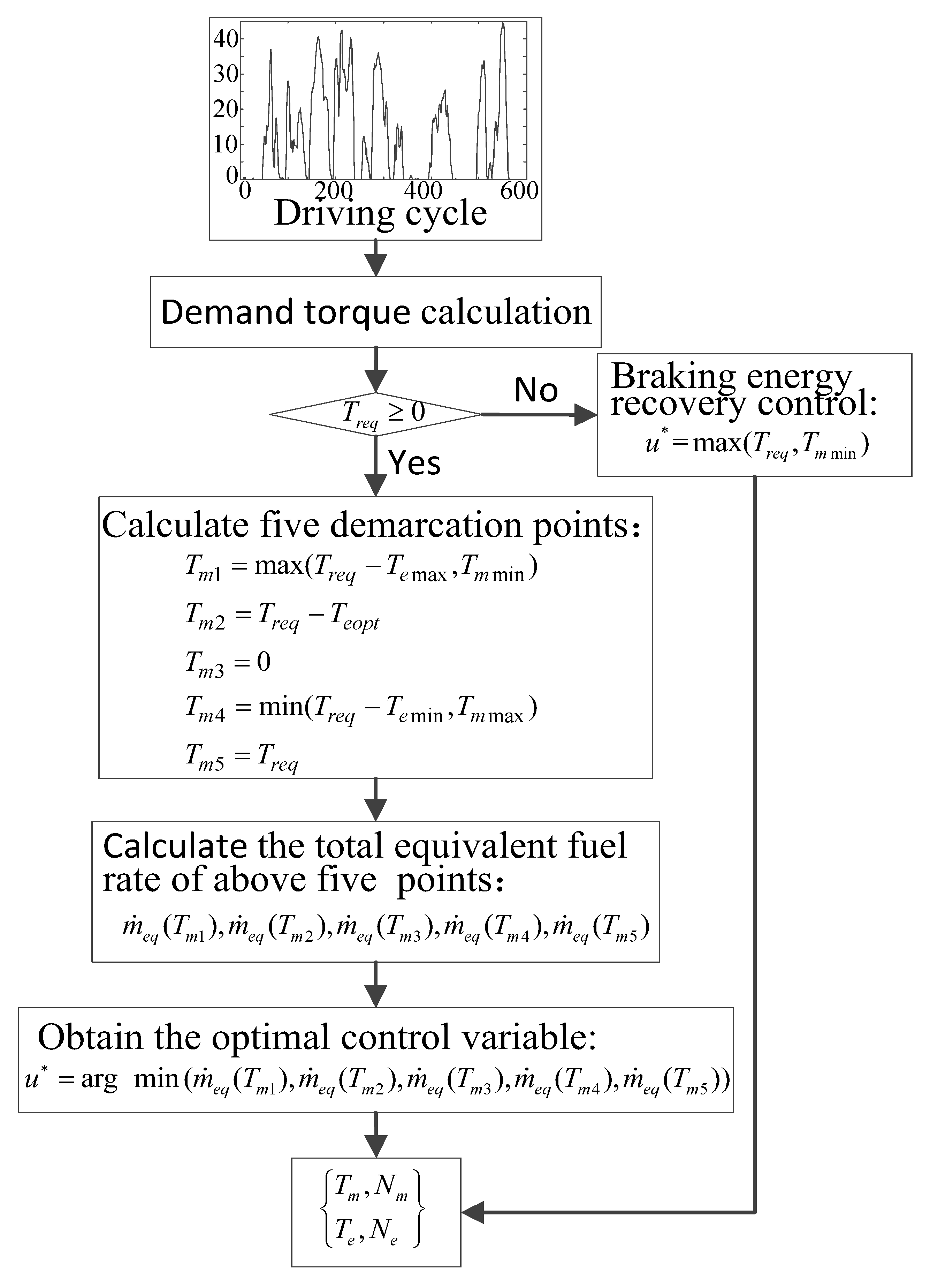
According to Equations (17) and (18), the total equivalent fuel rate is a piecewise function, which is composed of four continuous convex quadratic function. Based on the property of convex function, the total equivalent fuel rate is also a convex function, therefore the minimum value of the total equivalent fuel rate can only be obtained at points of the demarcation of the convex piecewise function. As shown in Equations (17) and (18), the demarcation points of the piecewise function are $T_m=\max (T_{req}-T_{\mathrm{e}\max },T_{\min })$,$T_m=T_{req}-T_{opt}$, $T_m=0$, $T_m=\min (T_{req}-T_{\mathrm{e}\min },T_{\max })$ and $T_m=T_{req}$. Thus, the optimal control variable can only be obtained from above five points. The optimal solution can be determined by comparing the value of the total equivalent fuel rate of the five points. Based on above conclusion, the simplified equivalent fuel consumption minimization strategy (Simplified-ECMS) is proposed.

The concept of the Simplified-ECMS is achieving the optimal solution by comparing the total equivalent fuel rate of above five points for each time instant, instead of comparing the values of every step point in the control domain, which is the principle of normal ECMS. Therefore, the Simplified-ECMS can greatly reduce the amount of calculation and shorten the time of calculation. The procedure flow chart of the Simplified-ECMS is shown in Figure 8.

To validate the effect of the Simplified-ECMS-based strategy, three energy management strategies are simulated under ten repeated NEDC driving cycles: CD-CS-based, ECMS-based and Simplified-ECMS-based. The initial SOC is set 0.95, the final SOC is set 0.25. The simulation is operated on a desktop computer with 4 gigabits of RAM and 2.3 GHz of core i3 processor. In this section, the equivalent factor is determined by trial and error method.

The simulated SOC variation trajectories under three control strategies mentioned above are shown in Figure 9, the figure shows that the SOC of Simplified-ECMS-based strategy and ECMS-based strategy declines with the increasing of driving distance, and it reaches the target SOC value at the driving end, these two SOC curves are close, which shows that the optimization effect of Simplified-ECMS-based strategy is very close to the ECMS-based strategy.

Figure 10 is the engine working points under three control strategies. According to the figure, most engine working points of Simplified-ECMS-based strategy coincide with the points of ECMS-based strategy, and these two strategies’ engine working points are almost in engine’s economic zone, while CD-CS-based strategy’s engine working points are only a few parts in the economic zone.

Table 2. Fuel consumption and calculation time under three control strategies.

Result	CD-CS	ECMS	Simplified-ECMS
fuel consumption (L)	4.812	3.964	3.967
calculation time * (s)	72.88	966.89	146.44
Final SOC	0.2502	0.250	0.2501

Note: * The calculation was completed on a desktop computer with 4 gigabits of RAM and 2.3 GHz of core i3 processor.

is the engine’s fuel consumption and calculation time of three control strategies under ten repeated NEDC driving cycles. The fuel consumption from the Simplified-ECMS-based strategy and the ECMS-based strategy are close, but the fuel consumption of the Simplified-ECMS-based strategy is obviously less than the consumption of the CD-CS-based strategy; the calculation time of the Simplified-ECMS-based strategy is obviously shorter than the ECMS-based strategy, it is close to the time of the CD-CS-based strategy, which is a real-time control strategy. Therefore, the Simplified-ECMS-based strategy can obtain excellent fuel economy, and can obviously shorten the calculation time. We can conclude that Simplified-ECMS-based strategy is more appropriate for real-time control than ECMS-based strategy.

5. Adaptive Simplified-ECMS-Based Strategy

The key for the implementation of the Simplified-ECMS-based strategy is to find the right equivalent factor, which is considered to be a balancer balancing electrical energy consumption and fuel energy consumption. A large number of scholars have conducted discussions about equivalent factor. There are mainly two kinds of equivalent factor were proposed, the fixed equivalent factor [24,26] and the adaptive equivalent factor. The former relies on prior knowledge about the driving cycle, which deters it from real-time implementation. The adaptive equivalent factor has fairly ideal performance. A commonly used approach for obtaining the adaptive equivalent factor is using a feedback controller, such as a PI controller [21,27], a fuzzy PI controller [28], a PID controller [29] and a fuzzy logic controller [30], this method mainly based on the SOC reference, which is calculated from the predicted driving horizon [25,31]. The parameters of the PI/PID and the law of fuzzy controller are hard to be chosen, and the computation load of fuzzy logic controller is still heavy, therefore, above feedback controllers are still difficult to be applied in the real vehicle. In this section, the equivalent factor optimization model is established, then, the equivalent factor is optimized off-line by the particle swarm optimization (PSO) genetic algorithm under different driving cycles, therefore, the best equivalent factor MAPs are obtained, finally, the adaptive Simplified-ECMS-based strategy is implemented based on the equivalent factor MAPs.

5.1. Equivalent Factor

As we known, the equivalent factor can be used to adjust the electrical energy consumption and fuel energy consumption. For example, if the SOC is high, more electrical energy is consumed by reducing the equivalent factor, otherwise, more fuel energy is consumed by increasing the equivalent factor. Based on knowing the preliminary change between the equivalent factor and the SOC, we can establish an initial function, which preliminarily defines above changes, and modify it according to different driving cycles, driving distances and initial SOC. The initial function is expressed as

$$\lambda (t,\mathrm{SOC})=k\cdot f(SOC)$$

(19)

where $f(SOC)$ is the initial function; $k$ is the correction coefficient of the initial function. The initial function is shown in Figure 11, as shown in the figure, the value of initial function increases with the decreasing of SOC, and the rate of increasing is different when the SOC in different regions. For example, when SOC is lower than 0.25, the value of the initial function increases fastest with the decreasing of SOC, which can defer SOC further declining.

5.2. Off-Line Optimization Based on PSO Algorithm

After determining the initial function, the equivalent factor entirely depends on the correction coefficient $k$, therefore, the energy distribution of the engine and the battery can be dynamically adjusted by only altering the correction coefficient $k$. Then, the correction coefficient $k$ becomes a key parameter of the adaptive Simplified-ECMS-based strategy, and the key parameter of this strategy is optimized by PSO algorithm because its optimization is a nonlinear global optimization process, the fitness function is expressed as

$$\{\begin{array}{l}F={\min }_{\left\{k\right\}}{\displaystyle {\int }_0^t{\dot{m}}_{ice}\left(\mathrm{t}\right)\mathrm{d}t}\\ 0.25\le SOC(\mathrm{t})\le 0.95\\ T_{\mathrm{emin}}(\mathrm{t})\le T_e(\mathrm{t})\le T_{\mathrm{emax}}(\mathrm{t})\\ T_{\mathrm{mmin}}(\mathrm{t})\le T_m(\mathrm{t})\le T_{\mathrm{mmax}}(\mathrm{t})\end{array}$$

(20)

The flow chart of $k$ optimization is shown in Figure 12, the simulation is performed under ten repeated NEDC driving cycles, the initial SOC is 0.95, the parameters of PSO are set: the size of particle swarm is 100, the maximum number of iterations is 100, the initial inertia weight 0.9, the final inertia weight is 0.4.

The optimization result is shown in Figure 13, the optimal value of $k$ is 4.38, and the optimal fuel consumption is 3.945 L. Comparison results of two equivalent factor determining methods are given in

Table 3. Comparison results of two equivalent factor determining methods.

Results	Equivalent Factor Determined by Trial and Error Method	Equivalent Factor Determined by PSO Algorithm	Saving
Fuel consumption (L)	3.967	3.945	0.55%
Final SOC	0.2501	0.2502	---

, the equivalent factor determining by PSO algorithm can saved fuel consumption by 0.55% compared to the trial and error method.

Equivalent factor is mainly affected by driving distance and initial SOC in certain driving cycle [32], then, based on Equation (19), correction coefficient $k$ is also mainly affected by the driving distance and the initial SOC in certain driving cycle, Above $k$ optimization is based on the given driving distance and initial SOC, Next, under NEDC driving cycle, the $k$ optimization is implemented one by one in different driving distance and initial SOC through off-line optimization, and the MAP figure of correction coefficient $k$ under the NEDC driving cycle, as shown in Figure 14, is obtained.

As shown in Figure 14, when the driving distance is less than the pure electric mileage, $k$ is a constant, and its value is minimum, the reason is that electrical energy is enough in this condition, a small $k$ makes driving using battery power as more as possible; when the driving distance is larger than the pure electric mileage, $k$ increases with the increasing driving distance in certain initial SOC, which can blend electric energy with the trip distance adding. $k$ reduces with the increasing initial SOC in certain driving distance, then, the opportunity of motor participation increases under this way.

5.3. Implementation of the Adaptive Simplified-ECMS-Based Strategy

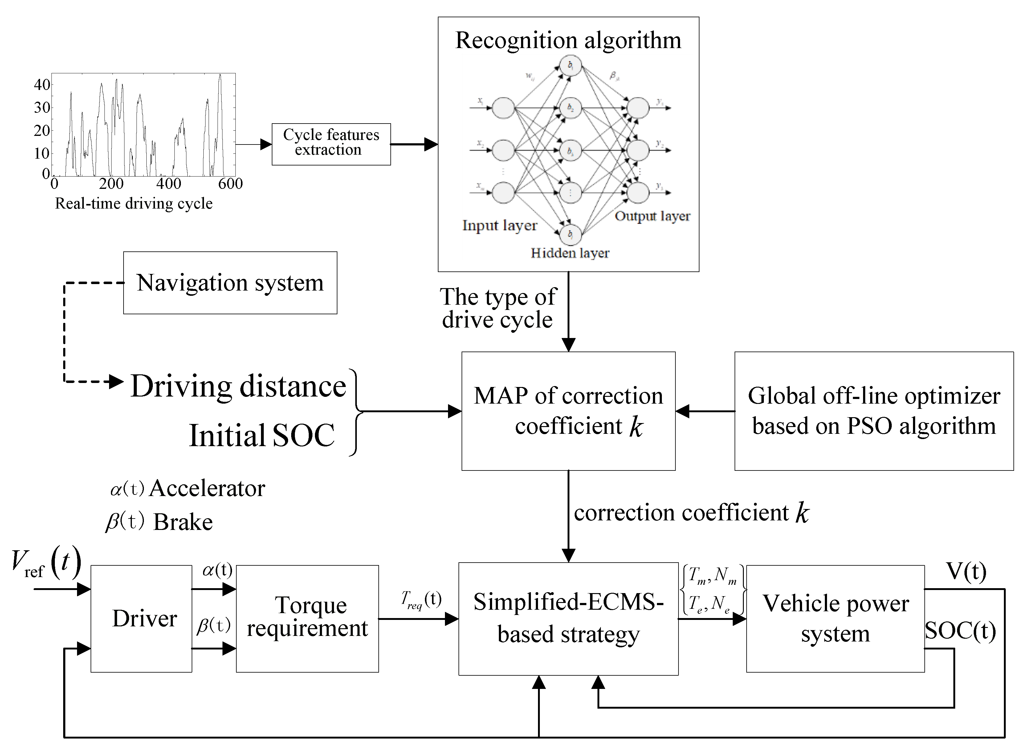
Determining the correction coefficient $k$ in actual driving conditions is a key issue for implementing adaptive Simplified-ECMS-based strategy. In the real-time control of PHEV, the $k$ could not be obtained by PSO algorithm on-line due to the great computational burden. However, the value of $k$ in different driving distances, initial SOC and driving cycles can be obtained by PSO algorithm off-line, which has been done in Section 5.2. Therefore, the control flowchart of the adaptive Simplified-ECMS-based strategy can be set in Figure 15. Firstly, the correction coefficient’s MAPs (like Figure 14) under different driving cycles are obtained by global off-line optimizer based on the PSO algorithm. Secondly, identify the type of the real driving cycle based on the recognition algorithm. Thirdly, the driving distance is gained by vehicle’s navigation system. Fourthly, extract the optimal correction coefficient $k$ from above MAPs through the obtained type of driving cycle, the driving distance and the initial SOC. Finally, Simplified-ECMS-based strategy is applied to distribute the engine and motor’s torque, and out put the optimal engine and motor’s torque to vehicle power system.

5.4. Simulation Validation of the Adaptive Simplified-ECMS-Based Strategy

Another key business for applying the adaptive Simplified-ECMS-based strategy is driving pattern recognition. Generally, the methods of the driving pattern or system recognition mainly include a fuzzy logic controller [33,34], cluster analysis [35], k-means clustering method [36], support vector machine (SVM) [37], extended support vector machine (SVM) [38], neural network [39], learning vector quantization network [40] and genetic programming (GP) for system recognition [41,42]. In this paper, extreme learning machine (ELM) is used for driving pattern recognition.

5.4.1. Driving Pattern Recognition Based on ELM

ELM is an easy and effective algorithm for single layer feed forward neural network, was first introduced by Huang et al. [43]. The structure of ELM model is shown in Figure 16.

The target of driving pattern recognition is to analyze the velocity information and classify practical driving patterns as similar standard driving cycles. Recognized driving cycles should be included in the representative driving cycle group. Six representative standard driving cycles, shown in

Table 4. Representative standard driving cycles.

Driving Cycle Type	Name	Driving Cycle Number
Urban Road	NYCC	Driving Cycle 1
	NewYorkBus	Driving Cycle 2
Suburb Road	ECE_EUDC_LOW	Driving Cycle 3
	UDDS	Driving Cycle 4
Highway Road	HWFET	Driving Cycle 5
	US06_HWY	Driving Cycle 6

and Figure 17, were selected in this paper to cover most of the different street types and driving behaviors. Therefore, in Figure 16, the output layer has six neurons that represent above six typical driving cycles. The input vector of the input layer is X = [x1, x2, …, x11], $w_{ij}$ is the weight between the ith neuron of the input layer and the jth neuron of the hidden layer. To identify the driving pattern, the eleven features were extracted from the vehicle speed during the time interval, and the eleven neurons of the input layer matched these eleven characteristic parameters: average speed ($\overline{v}$), maximum speed ($v_{\max }$), maximum acceleration ($a_{\max }$), average acceleration ($\overline{a}$), maximum deceleration ($d_{\max }$), average deceleration ($\overline{d}$), idle time factor $r_i$ (idle time/total time), acceleration time factor $r_a$ (acceleration time/total time), deceleration time factor $r_d$ (deceleration time/total time), uniform time factor $r_c$ (uniform time/total time) and idle times ($f_i$).

The training samples can be obtained based on characteristic parameters of the six typical driving cycles. If only the characteristic parameters of whole driving cycle are taken as training samples, the accuracy of training and recognition is difficult to guarantee for too little sample data. Therefore, it is preferable to divide each driving cycle into the appropriate number of 120 s overlapping shorter periods and then to extract their characteristic parameters.

Table 5. Recognition characteristics of the six typical driving cycles.

Driving Cycle	$\overline{\mathit{v}}$	${\mathbf{v}}_{\mathbf{max}}$	${\mathit{a}}_{\mathit{m}\mathit{a}\mathit{x}}$	$\overline{\mathit{a}}$	${\mathit{d}}_{\mathit{m}\mathit{a}\mathit{x}}$	$\overline{\mathit{d}}$	${\mathit{r}}_{\mathit{i}}$	${\mathit{r}}_{\mathit{a}}$	${\mathit{r}}_{\mathit{d}}$	${\mathit{r}}_{\mathit{c}}$	${\mathit{f}}_{\mathit{i}}$
1	11.41	44.6	2.68	0.62	−2.64	−0.64	0.351	0.326	0.304	0.020	18
1	7.07	36.9	2.50	0.74	−2.06	−0.72	0.433	0.283	0.258	0.025	5
1	22.64	42.5	2.68	0.68	−2.64	−0.63	0.033	0.442	0.483	0.042	2
1	10.23	36.1	2.24	0.62	−1.39	−0.54	0.308	0.325	0.358	0.008	4
1	6.26	25.4	1.43	0.38	−1.48	−0.47	0.542	0.242	0.192	0.025	5
1	10.84	44.6	1.83	0.62	−2.49	−0.90	0.437	0.336	0.227	0.000	2
1	16.45	40.6	2.50	0.70	−2.06	−0.58	0.108	0.408	0.458	0.025	3
1	19.04	42.5	2.68	0.77	−2.64	−0.65	0.142	0.383	0.433	0.042	3
1	6.04	22.1	1.61	0.50	−1.39	−0.58	0.433	0.292	0.258	0.017	5
1	8.81	33.8	1.48	0.46	−2.46	−0.71	0.417	0.333	0.242	0.008	3

shows the NYCC driving cycle divided into ten time periods. Using this method, characteristic parameters of the six driving cycles in different periods are taken as training samples.

Unlike conventional neural networks whose weights need to be tuned using the backpropagation algorithm, in ELM the weights between the input layer and the hidden layer and the biases of the hidden layer are randomly assigned. In default, sigmoid function is chosen as the activation function. Then, the ELM only needs to set the number of hidden layer nodes. In this work, this number is determined through gradually increasing the number of hidden neurons from 10 to 150 in interval of 10. The accuracy of recognition against the number of hidden neurons for ELM on the test sets, which is randomly extracted from training samples, is shown in Figure 18. It is seen that the highest accuracy has been achieved when the number of hidden neurons is between 70 and 100. In this paper, 80 hidden neurons are chosen to create the training model.

5.4.2. Simulation Validation of the Adaptive Simplified-ECMS-Based Strategy

To validate the effect of the adaptive Simplified-ECMS-based strategy, the CD-CS-based and the adaptive Simplified-ECMS-based strategy are simulated in Matlab/Simulink. The testing driving cycle, made up of Manhattan, SC03, UDDS, Japanese1015, WVUCITY and HWFET driving cycle, is structured in Figure 19a. The speed profiles from 0 to 1090 s, from 1090 to 1691 s, from 1691 to 3061 s, from 3061 to 3721 s, from 3721 to 5129 s, from 5129 to 5895 s, from 5895 to 7303 s, from 7303 to 8673 s, and from 8673 to 9763 s represent Manhattan, SC03, UDDS, Japanese1015, WVUCITY, HWFET, WVUCITY, UDDS, and Manhattan driving cycle, respectively. The speed profiles of Manhattan, SC03, UDDS, Japanese1015, WVUCITY and HWFET are obtained from ADVISOR (2002, National Renewable Energy Laboratory, Golden, CO, USA).

The ELM is used to identify the driving patterns, and the recognition result is shown in Figure 19b. From this result and combining with the speed curve of test driving cycle, ELM can recognize the types of the test driving cycle well. The simulation results of above strategies under the testing driving cycle are shown in Figure 20, Figure 21 and Figure 22, respectively.

Figure 20 is the SOC variation trajectories from the CD-CS-based and the adaptive Simplified-ECMS-based strategy. With the CD-CS-based strategy, the vehicle is driven mainly by electricity before it is fully depleted, so the SOC declines quickly in charge depleting stage, but the electrical energy of the vehicle, which is using the adaptive Simplified-ECMS-based strategy, is blended over the whole driving trip, therefore it can make the SOC dropping more slowly.

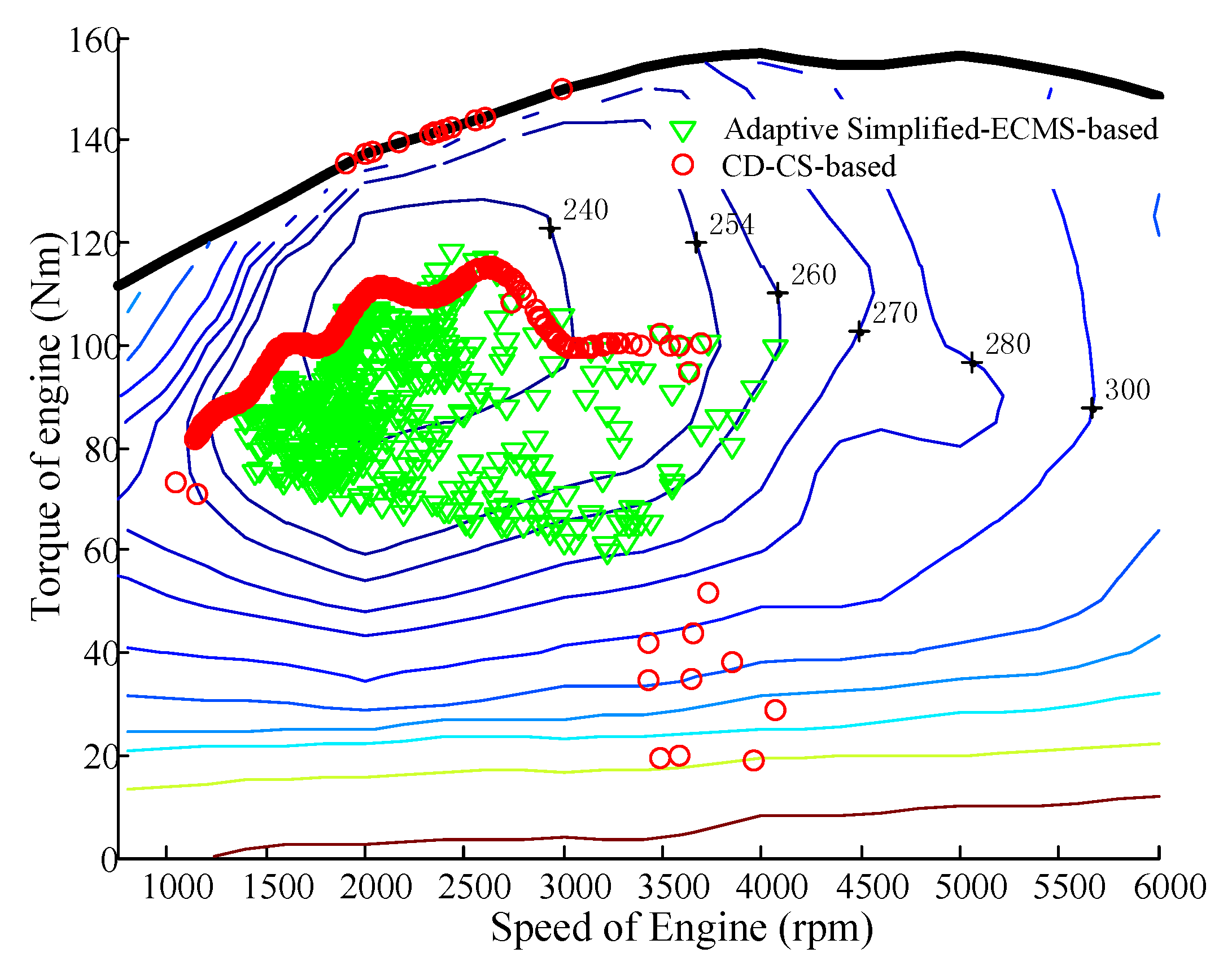
The engine operating points under the test driving cycle are shown in Figure 21. It can be seen that the adaptive Simplified-ECMS-based strategy intelligently controls engine in the low brake specific fuel consumption (BSFC) regions for any power level. In contrast, the CD-CS-based strategy operates the engine over a wider region. To some extent, the comparisons can prove that the proposed method can tune equivalent factor well according to the information of driving cycle, driving distance and initial SOC, and also can explain why the proposed method can save fuel consumption.

The fuel consumption variation trajectories from the CD-CS-based strategy and the adaptive Simplified-ECMS-based strategy are totally different, as shown in Figure 22. With the CD–CS-based strategy, the vehicle is driven almost completely by electricity before it is fully depleted, so the fuel consumption in the charge depletion stage is close to zero. Engine provides the main power after electricity is fully depleted, therefore, the fuel consumption increases rapidly after the charge depletion stage. However, the electrical energy is blended over the whole driving event when using the adaptive Simplified-ECMS-based strategy. Correspondingly, the fuel consumption accumulates with the increasing of the driving distance. The fuel consumption underthe CD-CS-based strategy is 1.874 L. The fuel consumption under the adaptive Simplified-ECMS-based strategy is 1.566 L, this strategy do help to reduce the fuel consumption significantly. The adaptive Simplified-ECMS-based strategy reduces the fuel consumption by 16.43% under the testing driving cycle, comparing to CD-CS-based strategy.

6. Road Test on the Prototype Vehicle

The Simplified-ECMS-based Strategy for PHEVs has been experimentally validated on a prototype PHEV. The parameters of the prototype vehicle are shown in Table 1. The prototype vehicle is shown in Figure 23. The vehicle’s control software is developed on the Development to Production (D2P, DEV+PROD, Germany E.ON, Essen, Germany) and Matlab/Simulink platforms.

The results of the road test have been presented in Figure 24. The velocity curve of the vehicle is shown in Figure 24a. The vehicle speed ranges from 0 to 61.58 km/h, the velocity of the test is low, the reason is that the prototype PHEV can only be tested on campus, for the sake of safety, the road test is only carried out at the low speed. The curves of five candidates’ total equivalent fuel rate are shown in Figure 24b. The driving modes include the start control mode (driving mode is equal to 0), the electric driving mode (driving mode is equal to 1), engine driving mode (driving mode is equal to 2), hybrid driving mode (driving mode is equal to 3), driving and charging mode (driving mode is equal to 4), and the regenerative braking mode (driving mode is 0.5). a1 is the start stage, so driving mode is equal to 0, the vehicle operates in the start control mode. In the a2 stage, $\min ({\dot{m}}_{eq}(T_{m1}),{\dot{m}}_{eq}(T_{m2}),{\dot{m}}_{eq}(T_{m3}),{\dot{m}}_{eq}(T_{m4}),{\dot{m}}_{eq}(T_{m5}))={\dot{m}}_{eq}(T_{m5})$ , this means the fifth candidate has the minimum total equivalent fuel rate. Therefore, the vehicle operates in the electric driving mode, and driving mode is equal to 1. Other stages can be analyzed in the same way. The engine and motor’s toque distribution during testing is shown in Figure 24c. The engine and motor’s total output torque’s response to the require torque is shown in Figure 24d, From the figure, the total output torque of the engine and motor tracks the require torque very well, which proves that the Simplified-ECMS-based Strategy can be applied to real time control completely.

7. Conclusions

The models of the engine’s fuel rate and battery’s consumption rate are approximately fitted by the piecewise function, which is made up of two quadratic functions. Then, the total equivalent fuel rate can also be expressed by piecewise function, which is a convex function actually. According to the properties of convex functions, the Simplified-ECMS-based strategy is proposed, this strategy only needs to calculate and compare five candidates’ total equivalent fuel rate to determine the optimal control for the Plug-in HEV.

CD-CS-based, ECMS-based and Simplified-ECMS-based strategies are simulated under ten repeated NEDC driving cycles, simulation results show that the Simplified-ECMS-based strategy can obtain excellent fuel economy, and shorten the calculation time obviously.

An initial function of the equivalent factor is established, then, searching the optimal equivalent factor converts to searching the optimal correction coefficient. After that, the parameter of the Simplified-ECMS-based strategy is optimized using the PSO algorithm, and the MAPs of this parameter under different driving patterns, driving distances and initial SOC are obtained.

Based on above MAPs, the adaptive Simplified-ECMS-based strategy is proposed, and the simulation is carried out to validate the control effect of this strategy. The simulation results show that the proposed strategy reduces the fuel consumption by 16.43% under the testing driving cycle, compared to CD-CS-based strategy.

Finally, the Simplified-ECMS-based strategy is validated on a prototype PHEV by a road test. The test results show that the Simplified-ECMS-based strategy can effectively distribute the engine torque and motor torque, and can be applied to real time control completely.

Currently, the adaptive Simplified-ECMS-based strategy is only verified through simulations. The next step is to perform hardware-in-the-loop test or experimental validations.

References

- Hu, X.; Martinez, C.M.; Yang, Y. Charging, power management, and battery degradation mitigation in plug-in hybrid electric vehicles: A unified cost-optimal approach. Mech. Syst. Signal Proc. 2017, 87, 4–16. [Google Scholar] [CrossRef]
- Akbari, M.; Brenna, M.; Longo, M. Optimal locating of electric vehicle charging stations by application of genetic algorithm. Sustainability 2018, 10, 1076. [Google Scholar] [CrossRef]
- Neyestani, N.; Damavandi, Y.; Godina, R.; Catalão, J.P.S. Integrating the PEVs’ traffic pattern in parking lots and charging stations in micro multi-energy systems. In Proceedings of the International Universities Power Engineering Conference, Coimbra, Portugal, 6–9 September 2016. [Google Scholar]
- Godina, R.; Paterakis, N.G.; Erdinc, O.; Rodrigues, E.M.G.; Catalão, J.P.S. Electric vehicles home charging impact on a distribution transformer in a portuguese island. In Proceedings of the 2015 International Symposium on Smart Electric Distribution Systems and Technologies (EDST), Vienna, Austria, 8–11 September 2015. [Google Scholar]
- Liu, X.; Wang, N.; Dong, D. A cost-oriented optimal model of electric vehicle taxi systems. Sustainability 2018, 10, 1557. [Google Scholar] [CrossRef]
- Hu, X.; Murgovski, N.; Johannesson, L.; Egardt, B. Energy efficiency analysis of a series plug-in hybrid electric bus with different energy management strategies and battery sizes. Appl. Energy 2013, 111, 1001–1009. [Google Scholar] [CrossRef]
- Kim, N.; Cha, S.; Peng, H. Optimal equivalent fuel consumption for hybrid electric vehicles. IEEE Trans. Veh. Technol. 2012, 20, 817–825. [Google Scholar]
- Gong, Q.; Li, Y.; Peng, Z.R. Computationally efficient optimal power management for plug-in hybrid electric vehicles with spatial domain dynamic programming. In Proceedings of the ASME 2008 Dynamic Systems and Control Conference, Ann Arbor, MI, USA, 20–22 October 2008. [Google Scholar]
- Yuan, Z.; Teng, L.; Fengchun, S. Comparative study of dynamic programming and Pontryagin’s minimum principle on energy management for a parallel hybrid electric vehicle. Energies 2013, 6, 2305–2318. [Google Scholar] [CrossRef]
- Chen, Z.; Mi, C.C.; Xu, J. Energy management for a power-split plug-in hybrid electric vehicle based on dynamic programming and neural networks. IEEE Trans. Veh. Technol. 2014, 63, 1567–1580. [Google Scholar] [CrossRef]
- Wang, X.; He, H.; Sun, F. Application study on the dynamic programming algorithm for energy management of plug-in hybrid electric vehicles. Energies 2015, 8, 3225–3244. [Google Scholar] [CrossRef]
- Martinez, C.M.; Hu, X.; Cao, D.; Velenis, E.; Gao, B.; Wellers, M. Energy Management in plug-in hybrid electric vehicles: Recent progress and a connected vehicles perspective. IEEE Trans. Veh. Technol. 2017, 66, 4534–4549. [Google Scholar] [CrossRef]
- Chen, Z.; Mi, C.C.; Xia, B. Energy management of power-split plug-in hybrid electric vehicles based on simulated annealing and Pontryagin’s minimum principle. J. Power Sources 2014, 272, 160–168. [Google Scholar] [CrossRef]
- Lin, X.; Banvait, H.; Anwar, S.; Chen, Y. Optimal energy management for a plug-in hybrid electric vehicle: Real-time controller. In Proceedings of the American Control Conference, Baltimore, MD, USA, 30 June–2 July 2010. [Google Scholar]
- Montazari-Gh, M.; Poursamad, A.; Ghalichi, B. Application of genetic algorithm for optimization of control strategy in parallel hybrid electric vehicles. J. Frankl. Inst. 2006, 343, 420–435. [Google Scholar] [CrossRef]
- Chen, Z.; Mi, C.C.; Xiong, R.; Xu, J. You, C. Energy management of a power-split plug-in hybrid electric vehicle based on genetic algorithm and quadratic programming. J. Power Sources 2014, 248, 416–426. [Google Scholar] [CrossRef]
- Hou, C.; Ouyang, M.; Xu, L. Approximate Pontryagin’s minimum principle applied to the energy management of plug-in hybrid electric vehicles. Appl. Energy 2014, 115, 174–189. [Google Scholar] [CrossRef]
- Xu, L.; Ouyang, M.; Li, J. Application of Pontryagin’s Minimal Principle to the energy management strategy of plugin fuel cell electric vehicles. Int. J. Hydrogen Energy 2013, 38, 10104–10115. [Google Scholar] [CrossRef]
- Sezer, V.; Gokasan, M.; Bogosyan, S. A novel ECMS and combined cost map approach for high-efficiency series hybrid electric vehicles. IEEE Trans. Veh. Technol. 2011, 60, 3557–3570. [Google Scholar] [CrossRef]
- Geng, B.; Mills, J.K.; Sun, D. Energy management control of microturbine-powered plug-In hybrid electric vehicles using the telemetry equivalent consumption minimization Strategy. IEEE Trans. Veh. Technol. 2011, 60, 4238–4248. [Google Scholar] [CrossRef]
- Nüesch, T.; Cerofolini, A.; Mancini, G.; Cavina, N.; Onder, C.; Guzzella, L. Equivalent consumption minimization strategy for the control of real driving NOx emissions of a diesel hybrid electric vehicle. Energies 2014, 7, 3148–3178. [Google Scholar] [CrossRef]
- Zhang, C.; Vahidi, A.; Pisu, P.; Li, X.; Tennant, K. Role of terrain preview in energy management of hybrid electric vehicles. IEEE Trans. Veh. Technol. 2010, 59, 1139–1147. [Google Scholar] [CrossRef]
- Egardt, B.; Murgovski, N.; Pourabdollah, M.; Mardh, L.J. Electromobility studies based on convex optimization: Design and control issues regarding vehicle electrification. IEEE Control Syst. Mag. 2014, 34, 32–49. [Google Scholar] [CrossRef]
- Paganelli, G.; Delprat, S.; Guerra, T.M.; Rimaux, J.; Santin, J.J. Equivalent consumption minimization strategy for parallel hybrid powertrains. In Proceedings of the IEEE 55th on Vehicular Technology Conference, Birmingham, AL, USA, 6–9 May 2002. [Google Scholar]
- Taghavipour, A.; Vajedi, M.; Azad, N.L. A comparative analysis of route-based energy management systems for PHEVs. Asian J. Control 2016, 18, 29–39. [Google Scholar] [CrossRef]
- Kim, N.W.; Lee, D.H.; Zheng, C.; Shin, C.; Seo, H.; Cha, S.W. Realization of pmp-based control for hybrid electric vehicles in a backward-looking simulation. Int. J. Automot. Technol. 2014, 15, 625–635. [Google Scholar] [CrossRef]
- Feng, T.H.; Yang, L.; Gu, Q.; Hu, Y.Q.; Yan, T.; Yan, B. A supervisory control strategy for plug-in hybrid electric vehicles based on energy demand prediction and route preview. IEEE Trans. Veh. Technol. 2015, 64, 1691–1700. [Google Scholar]
- Zhang, F.; Liu, H.; Hu, Y.; Xi, J. A supervisory control algorithm of hybrid electric vehicle based on adaptive equivalent consumption minimization strategy with fuzzy PI. Energies 2016, 9, 919. [Google Scholar] [CrossRef]
- Razavian, R.S. Design and evaluation of a real-time optimal control system for series hybrid electric vehicles. Int. J. Electr. Hybrid Veh. 2012, 4, 260–288. [Google Scholar] [CrossRef]
- Gupta, V. Energy management in parallel hybrid electric vehicles combining fuzzy logic and equivalent consumption minimization algorithms. HCTL Open Int. J. Technol. Innov. Res. 2014, 10. [Google Scholar]
- Rezaei, A.; Burl, J.B.; Zhou, B. Estimation of the ECMS equivalent factor bounds for hybrid electric vehicles. IEEE Trans. Control Syst. Technol. 2017, 99, 1–8. [Google Scholar] [CrossRef]
- Xie, S.; Li, H.; Xin, Z. A pontryagin minimum principle-based adaptive equivalent consumption minimum strategy for a plug-in hybrid electric bus on a fixed route. Energies 2017, 10, 1379. [Google Scholar] [CrossRef]
- Zhang, S.; Xiong, R. Adaptive energy management of a plug-in hybrid electric vehicle based on driving pattern recognition and dynamic programming. Appl. Energy 2015, 155, 68–78. [Google Scholar] [CrossRef]
- Chen, Z.; Xiong, R.; Cao, J. Particle swarm optimization-based optimal power management of plug-in hybrid electric vehicles considering uncertain driving conditions. Energy 2016, 96, 197–208. [Google Scholar] [CrossRef]
- Lei, Z.; Qin, D.; Liu, Y. Dynamic energy management for a novel hybrid electric system based on driving pattern recognition. Appl. Math. Model. 2017, 45, 940–954. [Google Scholar] [CrossRef]
- Montazeri-Gh, M.; Fotouhi, A. Traffic condition recognition using the k-means clustering method. Sci. Iran. 2011, 18, 930–937. [Google Scholar] [CrossRef]
- Liang, Z.; Xin, Z.; Yi, T. Intelligent energy management based on the driving cycle sensitivity identification using svm. In Proceedings of the 2009 2th International Symposium on Computational Intelligence and Design (ISCID’09), Changsha, China, 12–14 December 2009. [Google Scholar]
- Zhang, X.; Wu, G.; Dong, Z. Embedded feature-selection support vector machine for driving pattern recognition. J. Frankl. Inst. 2015, 352, 669–685. [Google Scholar] [CrossRef]
- Jeon, S.; Jo, S.; Park, Y. Multi-mode driving control of a parallel hybrid electric vehicle using driving pattern recognition. J. Dyn. Syst. Meas. Control 2002, 124, 141–149. [Google Scholar] [CrossRef]
- Langari, R.; Won, J.S. Intelligent energy management agent for a parallel hybrid vehicle-part I: System architecture and design of the driving situation identification process. IEEE Trans. Veh. Technol. 2005, 54, 925–934. [Google Scholar] [CrossRef]
- Garg, A.; Shankhwar, K.; Jiang, D.; Vijayaraghavan, V.; Panda, B.N.; Panda, S. An evolutionary framework in modelling of multi-output characteristics of the bone drilling process. Neural Comput. Appl. 2016, 10, 1233–1241. [Google Scholar] [CrossRef]
- Huang, Y.; Gao, L.; Yi, Z.; Tai, K.; Kalita, P.; Prapainainar, P.; Garg, A. An application of evolutionary system identification algorithm in modelling of energy production system. Measurement 2018, 114, 122–131. [Google Scholar] [CrossRef]
- Huang, G.B.; Zhu, Q.Y.; Siew, C.K. Extreme learning machine: Theory and applications. Neurocomputing 2006, 70, 489–501. [Google Scholar] [CrossRef] [Green Version]
Figure 1.
Parallel CVT-based PHEV powertrain system.