Seasonal Spatial Activity Patterns of Visitors with a Mobile Exercise Application at Seoraksan National Park, South Korea


1
Department of Tourism, Recreation and Sport Management, University of Florida, Gainesville, FL 32611-8208, USA
2
Cardiff Business School, College of Arts, Humanities & Social Sciences, Cardiff University, Aberconway Building, Colum Drive, Cardiff CF10 3EU, UK
*
Author to whom correspondence should be addressed.
Sustainability 2018, 10(7), 2263; https://doi.org/10.3390/su10072263
Submission received: 2 June 2018
/
Revised: 27 June 2018
/
Accepted: 27 June 2018
/
Published: 1 July 2018
(This article belongs to the Special Issue Agriculture, Landscape, Ecosystem Services and Biodiversity: New Challenges for Sustainable Development)
Abstract
:Visitors’ behavior in national parks can be influenced by seasonal variations in climate and preferred activities. Seasonality can produce different space consumption patterns, and impact visitor experience and natural resource use. The purpose of this study was to explore the seasonal spatial patterns of visitors’ activities using a mobile exercise application within the context of Seoraksan National Park in South Korea. A dataset composed of 5142 starting and ending points of 2639 activities (hiking and walking) created by 1206 mobile exercise application users (January–December 2015) were collected from a leading mobile exercise application operator. GIS-based spatial analytical techniques were used to analyze the spatial patterns of activity points across seasons and days (weekdays/weekends). Results indicated considerable seasonal and daily variations in activity distribution and hot spots (i.e., locations of potential congestion or crowding). The findings enable park managers to mitigate negative impacts to natural resources as well as enhance visitors’ experiences. Also, it allows potential visitors to decide when to visit certain sites via mobile application to ensure optimal conditions. Furthermore, the GPS-based exercise mobile application can be used as a new methodological approach to understand spatio-temporal patterns of visitors’ behavior within national parks and other natural protected areas.
1. Introduction
It is a global trend that natural protected areas, including national parks, have become major tourist attractions with eight billion annual visitors [1]. More specifically, national parks are valued by visitors due to the diverse recreation and tourism opportunities, as well as their natural and cultural resources [2,3]. With increasing demand and continual influx, park management agencies are faced with challenging options to develop more specific and measurable indicators that are central to management frameworks, and to ensure sustainable use that includes optimal visitor experience and resource protection (VERP) [4,5,6,7]. As noted by Manning [8], “indicators of quality are measurable, manageable variables that define the quality of visitor experiences and natural/cultural resources” (p. 93). Once standards and indicators of quality have been established, these can be monitored and managed within the scope of a park’s management plan to confirm that standards and indicators of quality are being preserved [9].
Tourism and recreational activities in national parks are seasonal phenomena due to climate variability that influences visitation [10,11,12]. Climate is an important factor in park-based tourism [6], as climate variability can influence physical resources that are considered tourist attractions [7]. Furthermore, visitors are very dependent on weather [13], as seasonal variation in conditions (e.g., temperature and wind) may affect activities and behaviors in national parks [14]. Seasonality can also have myriad negative impacts on the natural environment, as well as the visitor experience due to congestion or crowding issues, especially during the peak season [10,12,13]. Therefore, understanding seasonal patterns of park visitation is a prerequisite to forecast and manage park resources and enhance visitors’ experiences. As a result, several national park studies have examined the effects of seasonality on park visitation [10,11,14]. For example, Jones and Scott [10] studied seasonality and tourists’ visitation to Canada’s national parks, and identified expected increases due to an extended warm season, especially during the spring and fall seasons. Likewise, Scott et al. [11] also examined at Waterton Lakes National Park in Canada, and forecasted annual visitation to increase from 6% to 10% in the 2020s, and from 10% to 36% in the 2050s. In Australia, Hadwen et al. [14] identified key factors of seasonal visitation to 23 protected or natural parks across all six climate zones. They indicated that seasonal visits in equatorial, tropical, desert, grassland, and temperate zones were driven by climate, while visits to alpine and sub-alpine areas were influenced by natural and institutional factors (i.e., holiday periods).
Different seasonal visitation to tourist destinations, including national parks, generates seasonal activity areas which are popular during the high and off-season [12]. Even during the high season, differences in visitations and relevant activity areas might occur between weekdays and weekends [15]. Additionally, seasonal activity areas are based on the distributions of visitors’ activities. Thus, an examination of the seasonal spatial patterns of visitors’ activities in national parks is a managerial necessity to effectively manage congestion and/or crowding that are essential to optimize visitors’ experience. Furthermore, park managers should be able to provide visitors with useful information about seasonal and daily activity areas, such as visit and/or avoidance of certain areas under specific temporal conditions.
Prior studies have typically used global positioning system GPS-based tracking techniques to collect data on the spatio-temporal patterns of visitation in national parks and other tourist destinations [16,17,18,19,20,21,22]. Beeco et al. [16,17] used GPS tracking methods to assess the spatio-temporal patterns of visitor use, and identified the hot spots for runners, hikers, mountain bikers, and horseback riders in a local forest in Clemson, South Carolina, USA. Similarly, D’Antonio et al. [18] investigated the utility of GPS tracking methods to understand the spatio-temporal patterns of visitor use in various protected areas in the USA—Yosemite National Park, Bear Lake Corridor of Rocky Mountain National Park, and the Teton Range. Likewise, Hallo et al. [19] also noted the usefulness and functionality of GPS tacking methods, and assessed the spatial and temporal movement patterns of tourists in Sumter National Forest, USA. Lai et al. [20] used a GPS tracking method to assess visitors’ recreational tracking in Pokfulam County Park, Hong Kong. Similarly, Orellana et al. [21] used a GPS tracking method to analyze the spatio-temporal movement patterns of visitor flows in Dwingelderveld National Park, Netherlands. Collectively, these studies conclude that GPS-based tracking methods provide a more reliable, accurate, and precise dataset to describe visitor use patterns than traditional survey techniques.
Although GPS-based tracking methods have enabled researchers and practitioners to understand the spatio-temporal dimensions of visitors’ behavior, previous studies have not captured seasonal and spatial variability for an extended period due to limited sample sizes and short data collection periods. Furthermore, due to the limited battery life and data storage of tracking devices, previous GPS-based methods have noted difficulties in tracking visitors’ behavior within a backcountry or multi-day trip setting [20]. However, the recent introduction of GPS-based mobile applications such as outdoor health and exercise application has overcome the sampling and time constraints of traditional tracking methods [23]. Essentially, mobile exercise applications are software programs that work on mobile devices such as smartphones and tablet computers, and are intended to assist individuals to exercise systematically [24,25]. Specifically, the accurate and rich spatio-temporal data extracted from mobile exercise applications enable researchers to accurately determine visitors’ movement patterns across time and space, which compensates for the limitations in previous methods [26].
Due to the widespread use of smartphones, GPS-based mobile exercise applications, once activated by individual users can track app users’ real outdoor activities and generate accurate time and location information [23,26]. Given the potential benefits of a GPS-based mobile application, to the best of our knowledge, there is a lack of empirical research on its use and application for park management. Therefore, this study aimed to explore the seasonal and daily spatial patterns of visitors’ activities that were tracked and recorded by numerous mobile exercise application users at Seorakan National Park (SNP), South Korea. The findings of this study can assist park managers to better understand spatial variability of visitor flow across seasons and days, which further provides additional comprehensive seasonal geographic indicators to facilitate sustainable park management.
2. Materials and Methods
2.1. Study Area: Seoraksan National Park (SNP), South Korea
SNP is the fifth established national park, and is located within Inje Gun, Yangyang Gun, Sokcho Si, and Goseong Gun in Gangwon Province, South Korea. SNP was chosen as the study area because it is one of the most famous and highly visited parks, and is also a designated UNESCO Biosphere Reserve [27]. The distributions of attractions and visitor facilities inclusive of parking lots, campgrounds, information centers, and toilets, are illustrated in Figure 1. According to the Korean National Park Service [28], SNP attracted almost 4 million visitors in 2015, to experience a variety of natural and cultural attractions. Such a massive volume of visitation causes congestion and crowding that not only compromises visitors’ quality of experience, but also creates environmental impacts (i.e., soil erosion, damage to vegetation/heritage properties, water pollution, and increased fire frequency) [27,28]. Consequently, maintaining sustainability of park resources, along with ensuring visitors’ optimal experience, are key operational priorities of managers. Hence, this study can provide managers with a guideline to operate a more effective management system, and remedy resource damage from congestion and/or crowding at specific time periods (i.e., season and weekdays/weekends) and locations.
2.2. Data Collection
The GPS-based mobile application is regarded as an appropriate digital tracking technology that offer highly accurate and successive information about time and space [23,26]. This study used a depersonalized GPS-based mobile application dataset from “Tranggle”, which is the most popular outdoor mobile exercise application (https://www.tranggle.com) in South Korea. The depersonalized dataset maintains anonymity of all exercise application users, and the operator provides generalized data, including activity type, time, and the GPS coordinates of the place in which an activity occurs. Due to the numerous locational points for each activity, two points—starting and ending GPS coordinates—of one activity were extracted from the Tranggle database. The starting and ending points are the most important locational information for a specific hiking trail [29]. We assume that the starting point represents the point of interest for each activity, and its ending point can be similar to the point of origin—in the case of a round trip—or a different point—in the case of one-way trip. Most starting and ending points can be located on trails or across other places.
The final sample consisted of 2639 activities and 5142 starting and ending points—136 ambiguous outlier points located outside the study area were excluded from the initial 5278 points (2639 activities × 2 points)—recorded by 1206 participants from 1 January 2015 to 31 December 2015. The refined dataset showed that each participant, on average, visited SNP 2.19 times during the 1-year period. Most participants used the Tranggle app for hiking (2489, 94.3%), walking (106, 4.0%), jogging (19, 0.7%), bicycling (18, 0.7%) and other activities (7, 0.3%).
Such an activity dataset was exported into a point shape file (.shp) in a geographic information system (GIS). Nicholls [30] defined a shape file as a digital vector storage format for the geographical representation of a layer of spatial data. Geographic data, such as park boundaries and airphoto were downloaded from Biz-GIS, which supports spatial analysis and GIS applications for business and policy decisions in South Korea [31]. In this study, all GIS point shape files were projected and displayed in the Korean 1985 Katech (TM128) projection. It should be noted that the use of GIS-based mapping and spatial analysis is an evolving tool to understand visitors’ spatial behaviors in park and protected area settings [32].
2.3. Data Analysis
In order to identify seasonal activity areas, it is critical to define the optimal cell size to aggregate visitors’ activities that occur within a large park [33]. This study employed a 3 × 3 km cell as its unit of analysis based on Smallwood et al.’s [34] previous study. As a result, the study area included 69 cells. Figure 2 illustrates the locations of mountain trails, cell numbers and boundaries.
Since the seasonal spatial patterns of visitors’ activities encompasses an intricate process that requires a sequence of activities, a methodology flowchart for data analyses was formulated (see Figure 3).
Data analysis consisted of eight steps, which were implemented via ArcGIS (version 10.4.1., ESRI Redlands, NY, USA) and the ArcGIS Spatial Statistics Tool extension. All steps of seasonal spatial pattern analyses of visitors’ activities were also conducted during weekdays and weekends. First, to determine the seasonal activity patterns of visitors, 5142 point shape files were categorized based on season: spring (March–May), summer (June–August), fall (September–November), and winter (December–February). Second, the categorized point shape files for each season were divided into weekdays (Monday–Friday) and weekends (Saturday–Sunday) to determine weekdays/weekends activity patterns of visitors.
Third, seasonal distribution of activity points was assessed. Specifically, the central tendency (i.e., mean center and median center) and distributional trend (i.e., standard deviational ellipse) were measured. Spatial centrographic analysis and standard deviational ellipse analysis were used to measure and compare the seasonal mean centers, median centers, and standard deviational ellipses.
Fourth, nearest neighbor analysis (NNA) was used to explore the spatial patterns of activity points by calculating a nearest neighbor ratio (NNR). NNR is defined as the ratio of the observed mean distance to the expected mean distance between the features [35,36,37]. According to Wall et al. [38], the point pattern reveals a clustered distribution when the value of NNR is less than 1. If the value of NNR is greater than 1, the point pattern indicates a regular distribution. If the value of NNR is 1, the point pattern exhibits complete spatial randomness (CSR).
Fifth, the study area with 69 cells (3 × 3 km) and all point shape files in each cell were aggregated. This step was a prerequisite for the subsequent spatial autocorrelation and hot spot analyses of seasonal activity areas. Sixth, spatial autocorrelation analyses via global Moran’s I statistic were used to reveal the seasonal spatial patterns of activity areas. Global Moran’s I statistic has been commonly used to measure spatial clustering [39] based on Tobler’s First Law of Geography [40]. The global Moran’s I statistic is measured as follows:
where wij is the connectivity spatial weight between cell i and cell j (e.g., wij = 1 if cell i and cell j are adjacent; otherwise, wij = 0), xi is the number of activity points at cell i, xj is the number of activity points at cell j, μ is the average number of activity points, and N is the total number of cell units (in this study, n: 69). The range of global Moran’s I statistic lies between −1 and 1. A value of 1 exhibits a perfect positive autocorrelation, representing a pattern in which similar values occur in adjacent cells. A value of 0 exhibits CSR. A value of −1 exhibits a perfect negative autocorrelation, representing pattern in which high (or low) values are consistently located next to low (high) values [39,41,42].
Seventh, Getis-Ord statistic (hereafter, statistic) was employed to identify where the significant hot spots of seasonal activity were located in the study area. The hot spot analysis using the statistic has been commonly used in urban studies, particularly to identify significant hot spots of traffic accidents [43] or crime [44]. This approach has also been recently applied in tourism research [45]. The analysis was also based on Tobler’s [40] First Law of Geography. As an index of local spatial autocorrelation, the statistic was appropriate to identify cluster structures of high or low concentration [46]. A simple equation of the statistic is noted as follows:
where is the statistic that addresses the spatial dependence of the number of activity points in cell i of all n (n = 69) cells, is the number of activity points for each cell j, is the weight value between cell i and cell j, and n is the total number of cells. The standardized statistic generates z-scores that illustrates the number of activity points by cell with either high or low cluster value. This occurs spatially, and also measures statistical significance. The Z () statistic is noted as follows:
The null hypothesis is CSR. If the Z() value is positive, the high values’ distribution is clustered more spatially. In contrast, if the Z() value is negative, the low values’ distribution is clustered more spatially [46]. Lastly, areas of potential congestion and crowding in SNP were identified.
3. Results
3.1. Seasonal Spatial Patterns of Visitors’ Activities
3.1.1. Pattern of Visitors’ Activities
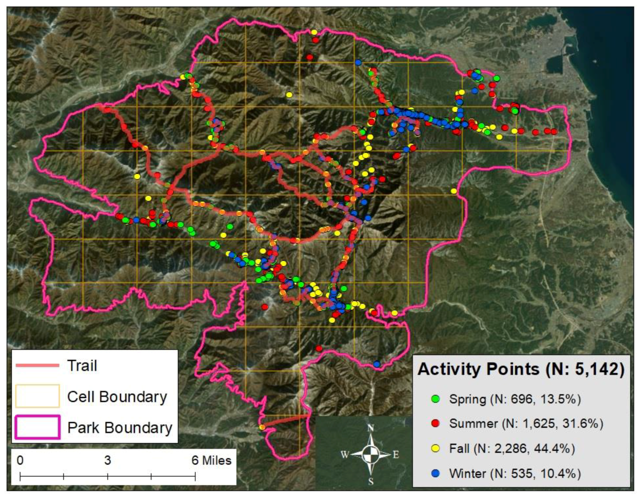
The seasonal distribution of activity points in SNP is illustrated in Figure 4. The largest number of activity points occurred in the fall season (September–November), while the smallest during the winter (December–February). More specifically, 696 (13.5%) of the 5142 activity points occurred in spring (March–May), 1625 (31.6%) in summer (June–August), 2286 (44.4%) in fall, and 535 (10.4%) in winter. These findings indicate the existence of seasonal effects of visitation in SNP (see Table 1). Furthermore, the starting and ending points of all activities were identified across and outside trails. The results demonstrate that visitors’ activities may start and end on the trails—which could be closely monitored by park authorities—or outside the trails, which poses challenges.
3.1.2. Central Tendency of Visitors’ Activities
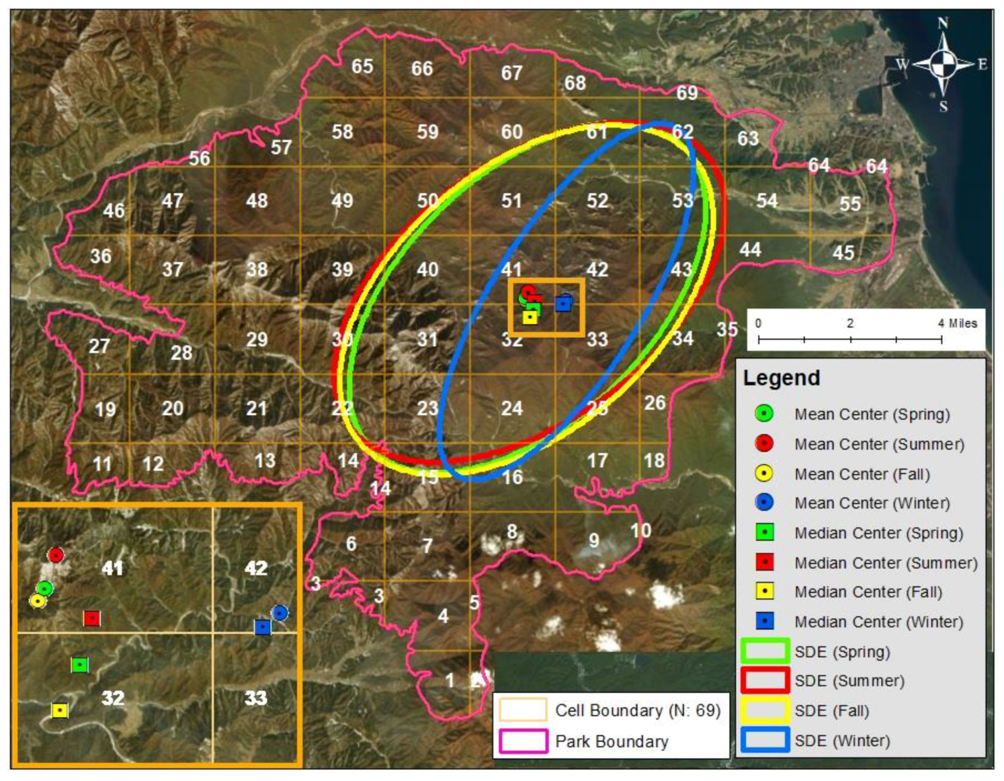
The mean and median centers for spring, summer, and fall were all located in cell 41 (i.e., mean centers for spring and fall; mean and median centers for summer) and cell 32 (i.e., median centers for spring and fall) (see Figure 5). However, the mean and median centers for winter were in cell 42. These findings indicate that while visitors’ activities during the winter were concentrated in the eastern region, they were mainly focused in the central region during the spring, summer, and fall seasons. In addition, standard deviational ellipses indicated that all seasonal distribution of activity points had a similar directional trend. Essentially, visitors’ seasonal activities were concentrated around the southwest axis in the northeast across all seasons. Table 2 reports that the largest area of standard deviational ellipse occurred in fall (44.01 sq mi), followed by those in summer (43.28 sq mi), spring (40.19 sq mi), and winter (22.82 sq mi). Thus, these results indicate the different seasonal spatial boundaries of visitors’ activities within SNP.
3.1.3. Point Patterns of Visitors’ Activities
The results of NNA for all seasonal distribution of activity points are summarized in Table 3. The values of NNR for all seasons were less than 1, which confirmed that the distribution of all seasonal activity points was significantly clustered.
3.1.4. Clustering of Activity Areas
Table 4 provides the values of global Moran’s I for seasonal activity areas (cells) across the 69 cells. The global Moran’s I values for all seasons were statistically significant (0.05 and 0.1 significance levels) and positive. These findings indicate positive spatial autocorrelation of seasonal activity areas that imply a tendency toward spatial clustering of seasonal activity areas whereby cells which exhibit high (or low) levels of visitors’ activity tend to be situated next to cells with similarly high (or low) levels of visitors’ activity.
3.1.5. Activity Hot Spots
The location and type of seasonal activity hot spots are illustrated in Figure 6. The results are also reported in Table 5, which indicates change in the number of cells that exhibit each of the seven outcomes of hot spot analyses (hot spot [99%], hot spot [95%], hot spot [90%], cold spot [99%], cold spot [95%], cold spot [90%], and not statistically significant). Interestingly, only hot spots were identified; no cold spots existed.
Specifically, 7 out of 69 cells were statistically significant in spring, which indicated that 7 activity hot spots (99% [3], 95% [3], 90% [1]) existed during the spring season. The detailed tourist attractions are identified in each cell area as follows:
- Cell 8: Oknyeo Waterfall, Sasigol Valley.
- Cell 16: Osaek Spring, Geumgangmun, Jujeongol Valley, Yongso Waterfall.
- Cell 23: Soseung Waterfall, Hangyeryeong Hill.
- Cell 24: Seorak Waterfall, Dokjugol Valley.
- Cell 42: Yangpok Waterfall.
- Cell 52: Shinheungsa Valley, Gwongeumseong Peak, Geunganggul Cave, Waseondae Rock.
- Cell 61: Heundeulbawi Rock, Ulsanbawi Rock.
During the summer season, 7 cells were identified as activity hot spots. The summer hot spots were similar to the spring hot spots, except for cell 16. Basically, cell 16 was replaced by cell 31: where Geoncheongol Valley, Gwittaegicheong Peak, and Baekun Waterfall are located. In the fall season, the number of significant cells increased to 8, with the addition of cell 6 to the 7 hot spots of the summer, or cell 31 to the 7 hot spots of the spring. Overall, this suggests that visitors’ activity areas during the fall become wider than those during the spring and summer seasons. Finally, during the winter, a total of 6 significant cells were identified and cells 23 and 31 were no longer significant.
3.2. Seasonal Spatial Patterns of Visitors’ Activities during Weekdays and Weekends
3.2.1. Visitors’ Activities during Weekdays and Weekends
The distribution of activity points was obtained via sub-division of the temporal unit from season to two daily formats: weekdays (Monday–Friday) and weekends (Saturday–Sunday). The seasonal distribution of activity points during weekdays and weekends is summarized in Table 6.
Visitors’ activities were concentrated largely during weekends for all four seasons. From a daily perspective, among the 5142 activity points, the largest number of activity points (1316, or 25.5%) were observed during fall weekends, while the smallest number (180, or 3.5%) were identified for spring weekdays. Specifically, 516 (74.2%) of 696 activity points were observed during spring weekends, 1157 (71.2%) of 1625 during the summer, 1316 (57.5%) of 2286 for fall, and 318 (59.5%) of 535 for the winter season. These findings indicate that, although the weekend effects of visitation were illustrated through each season, they were more pronounced during the spring and summer than for the fall and winter.
3.2.2. Central Tendency of Visitors’ Activities during Weekdays and Weekends
Figure 7 illustrates that the seasonal central tendency of activity points varies during weekdays and weekends. For weekdays, the mean and median centers for spring, summer, and fall were all located in cell 41 (i.e., mean centers for spring, summer, and fall; median center for summer) and cell 32 (i.e., median centers for spring and fall). But, the mean and median centers for the winter were in cell 42. These findings indicate that while visitors’ activities during the spring, summer, and fall were concentrated in the central region, they were mostly focused in the east region during the winter.
For weekends, the mean and median centers for summer and fall were all located in cell 41 (i.e., mean centers for summer and fall) and cell 32 (i.e., median centers for summer and fall). But, the median centers for spring and winter were in cell 42 (i.e., median center for spring) and cell 33 (i.e., median center for winter). These findings indicate that while visitors’ activities in the summer and fall occurred in the central region, they were focused in the east region during the spring and winter. In addition, seasonal standard deviational ellipses during weekdays and weekends denoted that all seasonal distribution of activity points had a similar directional trend. Specifically, visitors’ seasonal activities were concentrated around the southwest axis in the northeast.
Areas of seasonal standard deviational ellipses during weekdays and weekends are summarized in Table 7. The largest area of standard deviational ellipse occurred during weekdays in the fall, while the smallest during weekdays during the winter season. For weekdays, the areas of seasonal standard deviational ellipses were 34.03 sq mi (spring), 44.38 sq mi (summer), 45.45 sq mi (fall), and 22.15 sq mi (winter). For weekends, the areas of seasonal standard deviational ellipses were 41.41 sq mi (spring), 42.19 sq mi (summer), 40.86 sq mi (fall), and 23.01 sq mi (winter). These findings also indicate the different seasonal spatial boundaries of visitors’ activities during weekdays and weekends. Specifically, visitors’ activities tend to be spatially distributed during weekdays in summer and fall, and weekends in spring and winter.
3.2.3. Point Patterns of Visitors’ Activities during Weekdays and Weekends
The results of NNA for all seasonal distributions of activity points during weekdays and weekends are summarized in Table 8. The values of NNR for all seasons during weekdays and weekends were less than 1, which implied that the distribution of all seasonal activities during weekdays and weekends were significantly clustered.
3.2.4. Clustering of Activity Areas during Weekdays and Weekends
Table 9 summarizes that the values of global Moran’s I for seasonal activity areas during weekdays and weekends across the 69 cells in the SNP. The global Moran’s I values for all seasons during weekdays and weekends were statistically significant (0.05 level: weekdays/weekends for summer and fall; 0.1 level: weekdays/weekends for spring and winter). These findings indicate positive spatial autocorrelation of activity areas across season and day. That is, there existed a tendency toward the spatial clustering of seasonal activity areas during weekdays and weekends in which cells that exhibited high (or low) levels of visitors’ activity intensity tended to be situated next to cells with similar high (or low) levels of visitors’ activity intensity.
3.2.5. Activity Hot Spots during Weekdays and Weekends
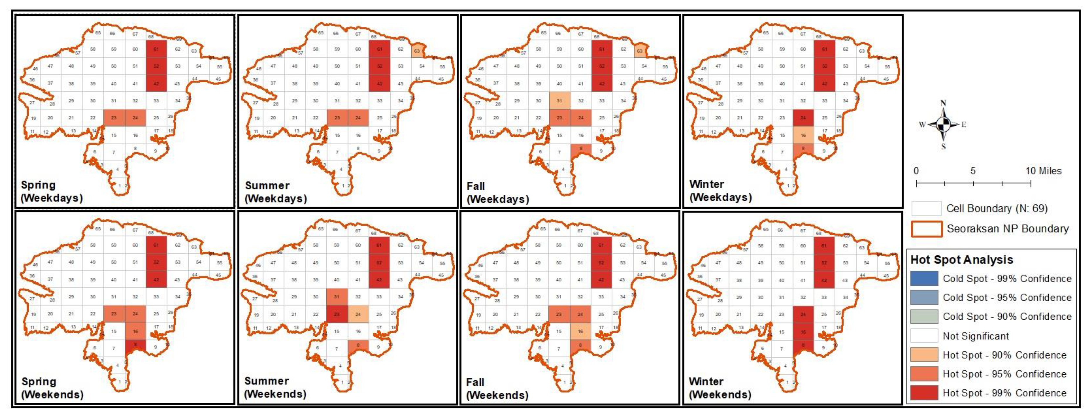
The location and type of seasonal activity hot spots during weekdays and weekends are illustrated and summarized in Figure 8 and Table 10, respectively. The number of significant activity hot spots during weekends were typically greater than those of weekdays hot spots. The findings indicated that weekend visitors were located densely in more areas. Although there were some differences in the location of activity hot spots between weekdays and weekends for all four seasons, the results were similar to those of the seasonal activity hot spots. Seasonal activity hot spots during weekdays and weekends were also identified (see Table 11). Cells 24, 42, 52, and 61 were the most visited hot spot areas both across the four seasons and during weekdays and weekends, while cell 63 was visited mostly during summer weekdays only.
3.3. Summary of Results
Table 12 summarizes the analysis techniques and findings related to the seasonal spatial patterns of visitors’ activities in SNP. The results indicated robust seasonal effects of visitation, and considerable seasonal variations in activity distribution and relevant hot spots. These findings were identified from two temporal perspectives: (1) seasonal and (2) mixed with season and day (weekdays and weekends).
4. Discussion and Implications
4.1. Discussion
Using a GPS-based mobile exercise application dataset, this study examined the seasonal spatial patterns of visitors’ activities in SNP, South Korea. To achieve this purpose, several GIS-based spatial analytical techniques were used to explore the seasonal spatial patterns of activity points and areas during weekdays and weekends. As illustrated in Table 1, there were seasonal effects of visitors’ activity and visitation, with the fall season (September–November) as the peak season. This finding could be explained by the ‘fall foliage’ effect during the peak season. SNP has one of the best fall foliage sites in the country which begins in late September. Also, this park is the first fall foliage mountain site, and initially attracts most visitors [27,28]. Rich colors, in combination with plenty of natural (e.g., rocks, forests, wildlife, hot springs) and cultural (e.g., ancient Shilla-era temples) sites, make SNP as a main attraction during the fall season. According to a Korean national tourism survey (2016), September (about 12.9%) was the most popular month for domestic travel, and nature/landscape appreciation (about 26.7%) was one of the main activities during domestic travel. Such results also support the importance of seasonal effects on visitors’ activity and visitation. Furthermore, this seasonal variation of visitation is consistent with previous national park studies which have identified the influence of variation in climate and visitation [10,11]. For example, Jones and Scott [10] identified that climate not only influences tourism and recreation activities, but also the length of stay and quality of experience. Hence, findings of this study provide further evidence of a seasonality effect as illustrated in the context of SNP.
This study finds that there were considerable seasonal variations in activity distribution and relevant hot spots. As summarized in Table 12, the largest spatial activity boundary and number of activity hot spots occurred in the fall, while the smallest occurred during the winter season (also see Table 2 and Table 5). These findings could be explained by seasonal climate variability, which can influence visitors’ resource use and spatial behavior [10]. Furthermore, seasonal variation in weather conditions, including temperature and wind, can affect visitors’ spatial movement and behavior in national parks [14]. As shown in Table 11, seasonal variations in activity hot spots occurred in cell 16 (Osaek Spring/Jujeongol Valley), cell 31 (Geoncheongol Valley/Baekun Waterfall), and cell 63 (Jubongsan Peak). For instance, since cell 16 is very notable for hot spring and fall foliage; cell 16 was found to be frequently visited during spring, fall, and winter. The reason why cell 16 was not popular during the summer can be explained by the seasonal climate and safety issues. Specifically, the park management’s official website identifies Jujeongol valley in cell 16 as a dangerous area, where “rock falls” may occur due to heavy rains during the summer season. These empirical findings support Ahas et al.’s [12] argument that seasonality can produce different visitor space consumption patterns in parks and tourist destinations.
Another finding is that there were considerable variations in activity distribution and relevant hot spots between weekdays and weekends. This result could be explained by the weekend effects of outdoor activities. As individuals have elevated feelings of freedom and closeness during the weekends periods [47], they are more likely to engage in their preferred activities and spend time with friends and/or family members. Thus, different spatial activity boundaries and behaviors during weekdays and weekends might be associated with temporal contexts, as individuals tend to visit distant and larger parks. This study recommends that further studies could collect individual level data via a visitor survey to further understand how and why spatial variability of park visitors differs during weekdays and weekends.
4.2. Implications
This study provides several important implications to visitor experience and resource protection framework (VERP) that is essential for sustainable park management. Our findings reinforce the VERP framework, which was formulated by the U.S. National Park Service to protect park resources, as well as to optimize visitors’ experiences [48]. An essential purpose of protected areas, including a national park, is not only to protect and conserve biodiversity, but also to provide visitors an opportunity to experience and interact with natural and cultural resources [49]. Understanding the spatio-temporal patterns of visitation can contribute to visitor monitoring, as well as management of environmental impacts. Our framework is designed to explore the seasonal spatial patterns of visitors’ activities in SNP (Figure 3), and offers comprehensive measurements of the spatio-temporal park visitations which can be incorporated into the VERP framework. In addition, this research also extends the literature on park management and outdoor recreation. Prior park management studies have been limited to identify “how to maintain the quality of park resources and visitor experiences” based on contemporary park management or planning frameworks. However, our methodological framework has widened this research focus to encompass the spatio-temporal element.
This study also suggests that a GPS-based mobile exercise application can help park managers to monitor spatio-temporal information more accurately, such as specific locations of visitors and density at a specific site. Such in-depth monitoring and predictive analytics are only possible via the use of ordinary visitors’ real-time activity data. For instance, accumulated visitors’ movement data can provide an important ‘early warning’ indicator of crowding and other issues experienced during a certain time and place [19]. Figure 9 illustrates the potential congestion or crowding of parts of the study area (A: Heundeulbawi Rock to Ulsanbawi Rock; B1: Min Park to Shinheung Temple; B2: Mini Park to Gwongeumseong; C: Huiungak Shelter Area; D: Huiungak Shelter to Daecheongbong; E: Osaek Spring Area).
Figure 10 further illustrates the spatial distribution of visitors’ activity density and risky points. The Korean National Park Service defines risky points as being related to falling-rocks, risk of structure collapse, or lightning. As of 2016, 33 risky points existed in SNP. By overlapping the density of visitors’ activities and risky points, park management can identify the specific locations of potential risky trails or warning areas (e.g., Osaek Spring Area in SNP). That is, based on the spatio-temporal visitation information, managers can establish a visitor management framework and control visitors’ resource use in SNP to ensure safety. For instance, park visitations can be controlled in the identified congested or warning areas when forest fires occur frequently (spring and fall), heavy rains (summer), or heavy snow falls (winter). Lastly, information on the seasonal hot spots of park visitors during weekdays and weekends also can provide locations with potential congestion or crowding issues per daily basis (e.g., weekdays and weekends).
The findings of this study also can be applied, along with the national park visitor information system designed to enhance visitors’ experience with a predictive geographical insight into which locations are crowded during a specific season and day. The quality of visitors’ experience is compromised due to crowdedness, and seasonality is a key critical component to assess in national parks [5,8,10]. Essentially, access to information can encourage enhanced action [50]. Therefore, information about park visitors’ activity hot spots (i.e., locations of potential congestion or crowding) across different seasons and days allow visitors to decide whether to visit specific sites at a specific time via GPS-based mobile application (see Figure 11). The use of GPS-based mobile application offers visitors a viable opportunity to compile useful real-time data information as it highlights locations where potential crowding and congestion may occur.
Because park visitors’ behavior can be influenced by seasonal variations in climate and preferred activities [10,11], information of seasonal activity hot spots during weekdays and weekends can also contribute to monitoring systems designed to protect natural and historic/cultural resources. Such information may be utilized by management agencies to allocate financial budgets and human resources more effectively by pinpointing the locations of congestion and/or crowded sites (see Figure 12). To achieve a balance between conservation and use of resources, park management also need to determine why visitors use certain sites or resources less frequently during a particular season(s).
As the preferences and activities of park visitors change over time, the findings of this study could provide insights for current and future planning/management to ensure sustainability of the park and its environmental resources. Within this context, the determination of existing visitors’ preferred sites enables managers to understand potential preferences of visitors, as well as implement dispersal initiatives to minimize pressure on specific locations that are routinely or seasonally crowded [51].
This study has implications to mitigate potential visitor conflicts in national parks. The management of conflict is important, as visitors’ activities tend to spatially coincide [52]. In addition, if visitors’ activities and the natural environment are not properly managed, conflict might occur among/between visitor groups and other stakeholders [53,54]. Thus, understanding the sites preferred by visitors should be intensively managed.
5. Limitations and Future Studies
Despite the methodological and practical implications of this study, several limitations can be identified. First, the findings are limited to a single national park (SNP) and cannot be generalized. Park visitors’ activities can be affected by their level of access to preferred settings [55]. Each national park has its own color and specific settings that can create different seasonal spatial patterns of visitors’ flows and activities. So, future studies should be conducted in other types of park areas, such as marine protected areas to compare the seasonal spatial patterns of visitors’ activities with consideration of the heterogeneity of each type of national park. Second, this study was not able to identify activity hot spots at different times of the day. Spatio-temporal dynamics of park visitors’ flows can reveal different space consumption patterns at different times of day (morning, afternoon and evening) during weekdays and weekends. So, future research should focus to explore the spatio-temporal patterns of visitors’ activities at different times of the day during weekdays and weekends. Third, although this study identified the location of sites with potential crowding or congestion issues in SNP, the meaning of crowding or congestion was not clearly defined. Crowding issues are major concerns that management should investigate. In addition, crowding might occur with too many visitors simultaneously in one place or on a given day and time. Thus, future studies should quantitatively measure the level of crowding at different time scales. Fourth, this study was not able to identify visitors’ preferences for their recreational activities that are essential to establish long-term management plans. Hence, a survey-based data collection could be combined with GPS-based visitation data and GIS information for future research. Lastly, due to limited data availability, only two data points of one activity—starting and ending—were used for the analysis. This results in an exclusion of all the locational data of each activity. Therefore, future studies could incorporate detailed locational points during a specific activity journey, which could facilitate the formulation of a complete illustration of the spatio-temporal patterns of park visitations.
6. Conclusions
This exploratory study examined the seasonal spatial patterns of visitors’ activities in the SNP. Despite the importance to understand seasonal spatial patterns of visitors’ activities, to our knowledge, no empirical studies have been conducted in this line of inquiry. Based on the utility of a large dataset of GPS-based mobile exercise application users’ visitations, this study examined the seasonal spatial patterns of visitors’ activities via several geospatial analytical techniques (e.g., spatial centrographic analysis, NNA, spatial autocorrelation analysis, hot spot analysis and kernel density estimation), in combination with GIS-based mapping. Such a new methodological framework allows for more comprehensive measurements of visitors’ spatio-temporal behaviors in national parks. Results indicated that there were considerable seasonal and weekdays/weekends variations in activity distribution and areas. The findings can contribute to aspects of management, whose main goals are to protect park resources and enhance visitor experiences. The findings broaden the scope of research questions with additional spatio-temporal insights into visitors’ activities. The use of a GPS-based mobile application in combination with GIS-based spatial analytical techniques is an emerging area of research that has major significance for management in national parks and other protected areas. We hope that this study will stimulate park researchers and managers to levy additional emphasis to seasonal spatial activity patterns of visitors via GPS-based mobile application users.
Author Contributions
All authors conceived and designed the research. J.K. and B.T. wrote Section 1, Section 2.2, Section 2.3, Section 3.1, Section 3.2, Section 5 and Section 6. S.J. collected the dataset and wrote Section 4. E.Y. analyzed the data and wrote Section 2.1.
Funding
The authors received no specific funding for this work.
Acknowledgments
The authors are thankful to Chi-Kuk Jang, CEO of Tranggle, for providing a sample dataset of GPS-based outdoor mobile exercise application. In addition, publication of this article was funded by the University of Florida Open Access Publishing Fund.
Conflicts of Interest
The authors declare no conflict of interest.
References
- Balmford, A.; Green, J.M.H.; Anderson, M.; Beresford, J.; Huang, C.; Naidoo, R.; Walpole, M.; Manica, A. Walk on the wild side: Estimating the global magnitude of visits to protected areas. PLoS Biol. 2015, 13. [Google Scholar] [CrossRef] [PubMed]
- Espinosa, T.; Vaske, J.J.; Donnelly, M.P. The politics of U.S. National park unit creation: The influence of electoral competition, political control, and presidential election years. J. Park Recreat. Adm. 2017, 35, 113–122. [Google Scholar] [CrossRef]
- Thapa, B. Why did they not visit? Examining structural constraints to visit Kafue National Park, Zambia. J. Ecotour. 2012, 11, 74–83. [Google Scholar] [CrossRef]
- Gundersen, V.; Mehmetoglu, M.; Inge Vistad, O.; Andersen, O. Linking visitor motivation with attitude towards management restrictions on use in a national park. J. Outdoor Recreat. Tour. 2015, 9, 77–86. [Google Scholar] [CrossRef] [Green Version]
- Manning, R.; Lawson, S.; Valliere, W. Multiple manifestations of crowding in outdoor recreation: A study of the relative importance of crowding-related indicators using indifference curves. Leisure/Loisir 2009, 33, 637–658. [Google Scholar] [CrossRef]
- Chaminuka, P.; Groeneveld, R.A.; Selomane, A.O.; van Ierland, E.C. Tourist preferences for ecotourism in rural communities adjacent to Kruger National Park: A choice experiment approach. Tour. Manag. 2012, 33, 168–176. [Google Scholar] [CrossRef]
- Trakolis, D. Perceptions, preferences, and reactions of local inhabitants in Vikos-Aoos National Park, Greece. Environ. Manag. 2001, 28, 665–676. [Google Scholar] [CrossRef] [PubMed]
- Manning, R. Visitor experience and resource protection: A framework for managing the carrying capacity of national parks. J. Park Recreat. Adm. 2001, 19, 93–108. [Google Scholar]
- Newman, P.; Manning, R.; Dennis, D.; McKonly, W. Informing carrying capacity decision making in Yosemite National Park, USA using stated choice modeling. J. Park Recreat. Admi. 2005, 23, 75–89. [Google Scholar]
- Jones, B.; Scott, D. Climate change, seasonality and visitation to Canada’s National Parks. J. Park Recreat. Adm. 2006, 24, 42–62. [Google Scholar]
- Scott, D.; Jones, B.; Konopek, J. Implications of climate and environmental change for nature-based tourism in the Canadian Rocky Mountains: A case study of Waterton Lakes National Park. Tour. Manag. 2007, 28, 570–579. [Google Scholar] [CrossRef]
- Ahas, R.; Aasa, A.; Mark, Ü.; Pae, T.; Kull, A. Seasonal tourism spaces in Estonia: Case study with mobile positioning data. Tour. Manag. 2007, 28, 898–910. [Google Scholar] [CrossRef]
- Reimann, M.; Lamp, M.-L.; Palang, H. Tourism impacts and local communities in Estonian National Parks. Scand. J. Hosp. Tour. 2011, 11, 87–99. [Google Scholar] [CrossRef]
- Hadwen, W.L.; Arthington, A.H.; Boon, P.I.; Taylor, B.; Fellows, C.S. Do climatic or institutional factors drive seasonal patterns of tourism visitation to protected areas across diverse climate zones in Eastern Australia? Tour. Geogr. 2011, 13, 187–208. [Google Scholar] [CrossRef]
- Pelletier, F. Effects of tourist activities on ungulate behaviour in a mountain protected area. J. Mt. Ecol. 2006, 8, 15–19. [Google Scholar]
- Beeco, J.A.; Hallo, J.C.; English, W.R.; Giumetti, G.W. The importance of spatial nested data in understanding the relationship between visitor use and landscape impacts. Appl. Geogr. 2013, 45, 147–157. [Google Scholar] [CrossRef]
- Beeco, J.A.; Hallo, J.C.; Brownlee, M.T.J. GPS Visitor tracking and recreation suitability mapping: Tools for understanding and managing visitor use. Landsc. Urban Plan. 2014, 127, 136–145. [Google Scholar] [CrossRef]
- D’Antonio, A.; Monz, C.; Lawson, S.; Newman, P.; Pettebone, D.; Courtemanch, A. GPS-based measurements of backcountry visitors in parks and protected areas: Examples of methods and applications from three case studies. J. Park Recreat. Adm. Fall 2010, 28, 42–60. [Google Scholar]
- Hallo, J.C.; Beeco, J.A.; Goetcheus, C.; McGee, J.; McGehee, N.G.; Norman, W.C. GPS as a method for assessing spatial and temporal use distributions of nature-based tourists. J. Travel Res. 2012, 51, 591–606. [Google Scholar] [CrossRef]
- Lai, P.C.; Li, C.L.; Chan, K.W.; Kwong, K.H. An assessment of GPS and GIS in recreational tracking. J. Park Recreat. Adm. 2007, 25, 128–139. [Google Scholar]
- Orellana, D.; Bregt, A.K.; Ligtenberg, A.; Wachowicz, M. Exploring visitor movement patterns in natural recreational areas. Tour. Manag. 2012, 33, 672–682. [Google Scholar] [CrossRef]
- Ligtenberg, A.; Van Marwijk, R.; Moelans, B.; Kuijpers, B. Recognizing patterns of movements in visitor flows in nature areas. In Proceedings of the 4th International Conference on Monotoring and Management of Visitor Flows in Recreational and Protected Areas, Montecatini Terme, Italy, 14–19 October 2018; Raschi, A., Trampetti, S., Eds.; [Google Scholar]
- Korpilo, S.; Virtanen, T.; Lehvävirta, S. Smartphone GPS tracking—Inexpensive and efficient data collection on recreational movement. Landsc. Urban Plan. 2017, 157, 608–617. [Google Scholar] [CrossRef]
- Sama, P.R.; Eapen, Z.J.; Weinfurt, K.P.; Shah, B.R.; Schulman, K.A. An evaluation of mobile health application tools. JMIR mHealth uHealth 2014, 2, e19. [Google Scholar] [CrossRef] [PubMed]
- Litman, L.; Rosen, Z.; Spierer, D.; Weinberger-Litman, S.; Goldschein, A.; Robinson, J. Mobile exercise apps and increased leisure time exercise activity: A moderated mediation analysis of the role of self-efficacy and barriers. J. Med. Internet Res. 2015, 17, e195. [Google Scholar] [CrossRef] [PubMed]
- Yun, H.J.; Park, M.H. Time–space movement of festival visitors in rural areas using a smart phone application. Asia Pacific J. Tour. Res. 2015, 20, 1246–1265. [Google Scholar] [CrossRef]
- Seo, C.W.; Choi, T.Y.; Choi, Y.S.; Kim, D.Y. A study on wildlife habitat suitability modeling for Goral (Nemorhaedus caudatus raddeanus) in Seoraksan National Park. J. Korea Soc. Envir. Res. Tech. 2008, 11, 28–38. [Google Scholar]
- Korea National Park Service. Available online: http://english.knps.or.kr/ (accessed on 31 December 2017).
- Flax, M.; Kariwo, S.; Chamaillé, A.; Michaelis, S. The best hiking trails in Cape Town 2018. The Inside Guide. Available online: https://insideguide.co.za/cape-town/hiking-trails/ (accessed on 29 May 2017).
- Nicholls, S. Measuring the accessibility and equity of public parks: A case study using GIS. Manag. Leis. 2001, 6, 201–219. [Google Scholar] [CrossRef]
- Biz-GIS. Available online: http://www.biz-gis.com/?ckattempt=1 (accessed on 21 June 2018).
- Kidd, A.M.; D’Antonio, A.; Monz, C.; Heaslip, K.; Taff, D.; Newman, P. A GPS-based classification of visitors’ vehicular behavior in a protected area setting. J. Park Recreat. Adm. 2018, 36, 69–89. [Google Scholar] [CrossRef]
- Sidman, C.F.; Fik, T.J. Modeling spatial patterns of recreational boaters: Vessel, behavioral, and geographic considerations. Leis. Sci. 2005, 27, 175–189. [Google Scholar] [CrossRef]
- Smallwood, C.B.; Beckley, L.E.; Moore, S.A.; Kobryn, H.T. Assessing patterns of recreational use in large marine parks: A case study from Ningaloo Marine Park, Australia. Ocean Coast. Manag. 2011, 54, 330–340. [Google Scholar] [CrossRef] [Green Version]
- Mitchell, A. The ESRI Guide to GIS Analysis, Volume 1: Geographic Patterns and Relationships; ESRI: Redlands, CA, USA, 2005. [Google Scholar]
- Kim, J. Measuring the Equity of Recreation Opportunity: A Spatial Statistical Approach. Ph.D. Thesis, Michigan State University, East Lansing, MI, USA, 2015. Unpublished thesis. [Google Scholar]
- Rogerson, P. Statistical Methods for Geography: A Student’s Guide; Sage Publications Inc.: Thousand Oaks, CA, USA, 2001. [Google Scholar]
- Wall, G.; Dudycha, D.; Hutchinson, J. Point pattern analyses of accommodation in Toronto. Ann. Tour. Res. 1985, 12, 603–618. [Google Scholar] [CrossRef]
- Kang, S.; Kim, J.; Nicholls, S. National tourism policy and spatial patterns of domestic tourism in South Korea. J. Travel Res. 2014, 53, 791–804. [Google Scholar] [CrossRef]
- Tobler, W.R. A computer movie simulation urban growth in Detroit Region. Econ. Geogr. 1970, 46, 234–240. [Google Scholar] [CrossRef]
- Jang, S.; Kim, J.; von Zedtwitz, M. The importance of spatial agglomeration in product innovation: A microgeography perspective. J. Bus. Res. 2017, 78, 143–154. [Google Scholar] [CrossRef]
- Jang, S.; Kim, J. Remedying food policy invisibility with spatial intersectionality: A case study in the Detroit Metropolitan Area. J. Public Policy Mark. 2018, 37, 167–187. [Google Scholar] [CrossRef]
- Kingham, S.; Sabel, C.E.; Bartie, P. The impact of the “school run” on road traffic accidents: A spatio-temporal analysis. J. Transp. Geogr. 2011, 19, 705–711. [Google Scholar] [CrossRef]
- Craglia, M.; Haining, R.; Wiles, P. A comparative evaluation of approaches to urban crime pattern analysis. Urban Stud. 2000, 37, 711–729. [Google Scholar] [CrossRef]
- García-Palomares, J.C.; Gutiérrez, J.; Mínguez, C. Identification of tourist hot spots based on social networks: A comparative analysis of European metropolises using photo-sharing services and GIS. Appl. Geogr. 2015, 63, 408–417. [Google Scholar] [CrossRef]
- Getis, A.; Ord, J.K. The analysis of spatial association by use of distance statistics. Geogr. Anal. 1992, 24, 189–206. [Google Scholar] [CrossRef]
- Bertram, C.; Meyerhoff, J.; Rehdanz, K.; Wüstemann, H. Differences in the recreational value of urban parks between weekdays and weekends: A discrete choice analysis. Landsc. Urban Plan. 2017, 159, 5–14. [Google Scholar] [CrossRef]
- Manning, R.E.; Lime, D.W.; Hof, M.; Freimund, W.A. The visitor experience and resource protection (VERP) process: The application of carrying capacity to Arches National Park. Georg. Wrig. Forum. 1995, 12, 41–55. [Google Scholar]
- Schliephack, J.; Moyle, B.; Weiler, B. Visitor expectations of contact with staff at a protected site. Ann. Leis. Res. 2013, 16, 160–174. [Google Scholar] [CrossRef] [Green Version]
- Yang, B.; Madden, M.; Kim, J.; Jordan, T.R. Geospatial analysis of barrier island beach availability to tourists. Tour. Manag. 2012, 33, 840–854. [Google Scholar] [CrossRef]
- Moyle, B.D.; Scherrer, P.; Weiler, B.; Wilson, E.; Caldicott, R.; Nielsen, N. Assessing preferences of potential visitors for nature-based experiences in protected areas. Tour. Manag. 2017, 62, 29–41. [Google Scholar] [CrossRef]
- Wolf, I.D.; Brown, G.; Wohlfart, T. Applying public participation GIS (PPGIS) to inform and manage visitor conflict along multi-use trails. J. Sustain. Tour. 2018, 26, 470–495. [Google Scholar] [CrossRef]
- Albritton, R.; Stein, T.; Thapa, B. Exploring conflict and tolerance between and within off-highway vehicle recreationists. J. Park Recreat. Adm. 2009, 27, 54–72. [Google Scholar]
- Rossi, S.D.; Pickering, C.M.; Byrne, J.A. Not in our park! Local community perceptions of recreational activities in peri-urban national parks. Australas. J. Environ. Manag. 2016, 23, 245–264. [Google Scholar] [CrossRef]
- Manning, R.E. Diversity in a democracy: Expanding the recreation opportunity spectrum. Leis. Sci. 1985, 7, 377–399. [Google Scholar] [CrossRef]
Figure 1.
Study area.

Figure 2.
Cell number in SNP.

Figure 3.
Methodology flowchart.

Figure 4.
Seasonal distribution of activity points in SNP.

Figure 5.
Seasonal central tendency and direction of activity points in SNP.

Figure 6.
Spatial distribution of seasonal activity hot spots.

Figure 7.
Central tendency and direction of activity points during weekdays and weekends.

Figure 8.
Spatial distribution of activity hot spots during weekdays and weekends.

Figure 9.
Locations of potential congestion and/or crowding in SNP.

Figure 10.
Spatial distribution of visitors’ activity density and risky points in SNP.

Figure 11.
Real-time national park crowding information system using web GIS and smartphone.

Figure 12.
Type of seasonal activity hot spots.


Table 1.
Seasonal number of activity points in SNP (N = 5142).
| Season | Number of Activity Points (%) |
|---|---|
| Spring (March–May) | 696 (13.5%) |
| Summer (June–August) | 1625 (31.6%) |
| Fall (September–November) | 2286 (44.4%) |
| Winter (December–February) | 535 (10.4%) |
Table 2.
Seasonal area of standard deviational ellipse in SNP.
| Season | Area (Unit: sq mi) |
|---|---|
| Spring (March–May) | 40.19 |
| Summer (June–August) | 43.28 |
| Fall (September–November) | 44.01 |
| Winter (December–February) | 22.82 |
Table 3.
Summary of seasonal nearest neighbor analysis.
| Season | Observed MD | Expected MD | NNR | p-Value | Clustered |
|---|---|---|---|---|---|
| Spring (March–May) | 36.78 | 320.05 | 0.11 | <0.01 | Yes |
| Summer (June–August) | 36.21 | 238.50 | 0.15 | <0.01 | Yes |
| Fall (September–November) | 33.74 | 204.30 | 0.16 | <0.01 | Yes |
| Winter (December–February) | 51.92 | 344.32 | 0.15 | <0.01 | Yes |
Note. MD: Medan distance; NNR: Nearest neighbor ratio.
Table 4.
Global Moran’s I values for spatial autocorrelation of seasonal activity areas.
| Season | Global Moran’s I | p-Value | Clustered |
|---|---|---|---|
| Spring (March–May) | 0.06 | <0.1 | Yes |
| Summer (June–August) | 0.21 | <0.05 | Yes |
| Fall (September-November) | 0.19 | <0.05 | Yes |
| Winter (December–February) | 0.02 | <0.1 | Yes |
Table 5.
Results of seasonal activity hot spot analysis.
| Type of Cluster | z-Score | CI (p-Value) | Frequency (%) | |||
|---|---|---|---|---|---|---|
| Spring | Summer | Fall | Winter | |||
| Hot spot (High clustering + High value) | >2.58 | 99% (<0.01) | 3 (4.3) | 3 (4.3) | 3 (4.3) | 3 (4.3) |
| 1.96 ~ 2.58 | 95% (<0.5) | 3 (4.3) | 2 (2.9) | 3 (4.3) | 2 (2.9) | |
| 1.65 ~ 1.96 | 90% (<0.1) | 1 (1.4) | 2 (2.9) | 2 (2.9) | 1 (1.4) | |
| CSR | −1.65 ~ 1.65 | Not Significant | 62 (89.9) | 62 (89.9) | 61 (88.4) | 63 (91.3) |
| Cold spot (High clustering + Low value) | −1.96 ~ −1.65 | 90% (<0.1) | 0 (0.0) | 0 (0.0) | 0 (0.0) | 0 (0.0) |
| −2.58 ~ −1.96 | 95% (<0.05) | 0 (0.0) | 0 (0.0) | 0 (0.0) | 0 (0.0) | |
| <−2.58 | 99% (<0.01) | 0 (0.0) | 0 (0.0) | 0 (0.0) | 0 (0.0) | |
| Total (%) | 69 (100.0) | 69 (100.0) | 69 (100.0) | 69 (100.0) | ||
Note. CI: Confidence Interval; CSR: Complete Spatial Randomness.
Table 6.
Number of activity points during weekdays and weekends.
| Season | Day | Number of Activity Points (%) | Total (%) |
|---|---|---|---|
| Spring (March–May) | Weekdays | 180 (25.8%) | 696 |
| Weekends | 516 (74.2%) | (100.0) | |
| Summer (June–August) | Weekdays | 468 (28.8%) | 1625 |
| Weekends | 1157 (71.2%) | (100.0) | |
| Fall (September–November) | Weekdays | 970 (42.5%) | 2286 |
| Weekends | 1316 (57.5%) | (100.0) | |
| Winter (December–February) | Weekdays | 217 (40.5%) | 535 |
| Weekends | 318 (59.5%) | (100.0) |
Table 7.
Area of standard deviational ellipse across season and day.
| Season | Day | Area (sq mi) |
|---|---|---|
| Spring (March–May) | Weekdays | 34.03 |
| Weekends | 41.41 | |
| Summer (June–August) | Weekdays | 44.38 |
| Weekends | 42.19 | |
| Fall (September–November) | Weekdays | 45.45 |
| Weekends | 40.86 | |
| Winter (December–February) | Weekdays | 22.15 |
| Weekends | 23.01 |
Table 8.
Summary of nearest neighbor analysis during weekdays and weekends.
| Season | Day | Observed MD | Expected MD | NNR | p-Value | Clustered |
|---|---|---|---|---|---|---|
| Spring | Weekdays | 78.00 | 541.21 | 0.14 | <0.01 | Yes |
| Weekends | 40.38 | 360.17 | 0.11 | <0.01 | Yes | |
| Summer | Weekdays | 61.86 | 380.11 | 0.16 | <0.01 | Yes |
| Weekends | 45.67 | 280.79 | 0.16 | <0.01 | Yes | |
| Fall | Weekdays | 40.05 | 300.54 | 0.13 | <0.01 | Yes |
| Weekends | 46.73 | 225.98 | 0.20 | <0.01 | Yes | |
| Winter | Weekdays | 119.92 | 484.17 | 0.24 | <0.01 | Yes |
| Weekends | 53.89 | 416.10 | 0.12 | <0.01 | Yes |
Note. MD: Medan distance; NNR: Nearest neighbor ratio.
Table 9.
Global Moran’s I values for spatial autocorrelation of activity areas during weekdays and weekends.
Table 9.
Global Moran’s I values for spatial autocorrelation of activity areas during weekdays and weekends.
| Season | Day | Global Moran’s I | p-Value | Clustered |
|---|---|---|---|---|
| Spring (March–May) | Weekdays | 0.04 | <0.1 | Yes |
| Weekends | 0.05 | <0.1 | Yes | |
| Summer (June–August) | Weekdays | 0.15 | <0.05 | Yes |
| Weekends | 0.24 | <0.05 | Yes | |
| Fall (September–November) | Weekdays | 0.13 | <0.05 | Yes |
| Weekends | 0.21 | <0.05 | Yes | |
| Winter (December–February) | Weekdays | 0.01 | <0.1 | Yes |
| Weekends | 0.02 | <0.1 | Yes |
Table 10.
Results of activity hot spot analysis during weekdays and weekends.
| SC | z-Score | CI (p-Value) | Frequency (%) | |||||||
|---|---|---|---|---|---|---|---|---|---|---|
| Spring | Summer | Fall | Winter | |||||||
| WD | WE | WD | WE | WD | WE | WD | WE | |||
| Hot Spot (HC+HV) | >2.58 | 99% (<0.01) | 3 (4.3) | 3 (4.3) | 3 (4.3) | 4 (5.7) | 3 (4.3) | 3 (4.3) | 4 (5.7) | 6 (8.6) |
| 1.96~2.58 | 95% (<0.5) | 2 (2.9) | 1 (1.4) | 2 (2.9) | 2 (2.9) | 3 (4.3) | 3 (4.3) | 1 (1.4) | 0 (0.0) | |
| 1.65~1.96 | 90% (<0.1) | 0 (0.0) | 3 (4.3) | 1 (1.4) | 1 (1.4) | 2 (2.9) | 1 (1.4) | 1 (1.4) | 0 (0.0) | |
| CSR | −1.65~1.65 | NS | 64 (92.7) | 62 (89.9) | 63 (91.3) | 62 (89.9) | 61 (88.4) | 62 (89.9) | 63 (91.3) | 63 (91.3) |
| Total (%) | 69 (100.0) | 69 (100.0) | 69 (100.0) | 69 (100.0) | 69 (100.0) | 69 (100.0) | 69 (100.0) | 69 (100.0) | ||
Note. No cold spot was identified. SC: Spatial clustering; HC: High clustering; HV: High value; CI: Confidence interval; CSR: Complete spatial randomness; NS: Not significant; WD: Weekdays; WE: Weekends.
Table 11.
Seasonal activity hot spot during weekdays and weekends.
| Cell | Major Attraction | Spring | Summer | Fall | Winter | ||||
|---|---|---|---|---|---|---|---|---|---|
| WD | WE | WD | WE | WD | WE | WD | WE | ||
| 8 | Oknyeo Waterfall/Sasigol Valley | ● | ● | ● | ● | ● | ● | ||
| 16 | Osaek Spring/Jujeongol Valley | ● | ● | ● | ● | ||||
| 23 | Soseung Waterfall/Hangyeryeong Hill | ● | ● | ● | ● | ● | ● | ||
| 24 | Seorak Waterfall/Dokjugol Valley | ● | ● | ● | ● | ● | ● | ● | ● |
| 31 | Geoncheongol Valley/Baekun Waterfall | ● | ● | ||||||
| 42 | Yangpok Waterfall | ● | ● | ● | ● | ● | ● | ● | ● |
| 52 | Shinheungsa/Gwongeumseong Peak | ● | ● | ● | ● | ● | ● | ● | ● |
| 61 | Heundeulbawi Rock/Ulsanbawi Rock | ● | ● | ● | ● | ● | ● | ● | ● |
| 63 | Jubongsan Peak | ● | |||||||
Note. WD: Weekdays; WE: Weekends; Cells with no seasonal hot spots during weekdays and weekends are 1–7, 9–15, 17–22, 25–30, 32–41, 43–51, 53–60, 62, and 64–69.
Table 12.
Summary of seasonal spatial pattern analyses.
| Temporality | Type of Analysis | Analysis Technique (Figure and Table) | Findings |
|---|---|---|---|
| Seasonal | Distribution of Activity Points | Frequency (Figure 4, Table 1) | The largest number of activity points occurred during the fall, the smallest in the winter. |
| Seasonal | Central Tendency of Visitors’ Activities | Spatial Centrographic Analysis, Standard Deviational Ellipse Analysis (Figure 5, Table 2) | The largest area of standard deviational ellipse occurred in the fall, followed by summer, spring, and winter. |
| Seasonal | Point Patterns of Visitors’ Activities | Nearest Neighbor Analysis (Table 3) | The distribution of all seasonal activity points was significantly clustered. |
| Seasonal | Clustering of Activity Areas | Spatial Autocorrelation Analysis (Table 4) | There existed a tendency towards the spatial clustering of seasonal activity areas such as hot spots and cold spots. |
| Seasonal | Activity Hot Spots | Spatial Hot Spot Analysis (Figure 6, Table 5) | 7 out of 69 cells belonged to the activity hot spots in the spring and summer, 8 in fall and 6 in the winter. |
| Seasonal + Daily | Distribution of Activity Points | Frequency (Table 6) | Visitors’ activities were concentrated largely during weekends for all four seasons. |
| Seasonal + Daily | Central Tendency of Visitors’ Activities | Spatial Centrographic Analysis, Standard Deviational Ellipse Analysis (Figure 7, Table 7) | The largest area of standard deviational ellipse occurred during weekdays in the fall, while the smallest during weekdays in the winter. |
| Seasonal + Daily | Point Patterns of Visitors’ Activities | Nearest Neighbor Analysis (Table 8) | The distribution of all seasonal activities during weekdays and weekends were significantly clustered. |
| Seasonal + Daily | Clustering of Activity Areas | Spatial Autocorrelation Analysis (Table 9) | There existed a tendency toward the spatial clustering of seasonal activity areas during weekdays and weekends. |
| Seasonal + Daily | Activity Hot Spots | Spatial Hot Spot Analysis (Figure 8, Table 10, Table 11) | The number of significant activity hot spots during weekends was greater than hot spots for the weekdays. |
© 2018 by the authors. Licensee MDPI, Basel, Switzerland. This article is an open access article distributed under the terms and conditions of the Creative Commons Attribution (CC BY) license (http://creativecommons.org/licenses/by/4.0/).
Share and Cite
MDPI and ACS Style
Kim, J.; Thapa, B.; Jang, S.; Yang, E. Seasonal Spatial Activity Patterns of Visitors with a Mobile Exercise Application at Seoraksan National Park, South Korea. Sustainability 2018, 10, 2263. https://doi.org/10.3390/su10072263
AMA Style
Kim J, Thapa B, Jang S, Yang E. Seasonal Spatial Activity Patterns of Visitors with a Mobile Exercise Application at Seoraksan National Park, South Korea. Sustainability. 2018; 10(7):2263. https://doi.org/10.3390/su10072263
Chicago/Turabian StyleKim, Jinwon, Brijesh Thapa, Seongsoo Jang, and Eunjung Yang. 2018. "Seasonal Spatial Activity Patterns of Visitors with a Mobile Exercise Application at Seoraksan National Park, South Korea" Sustainability 10, no. 7: 2263. https://doi.org/10.3390/su10072263
Note that from the first issue of 2016, this journal uses article numbers instead of page numbers. See further details here.