The Effect of Environmental Regulation on Employment in China: Empirical Research Based on Individual-Level Data

Abstract

This paper argues that the scale effect and substitution effect in the labor demand for environmental regulations should not be ignored in the pursuit of environmental improvements. It is necessary to analyze the influential mechanism of environmental regulations on employment. Based on the pooled cross-section data combined by CHIP (Chinese Household Income Project) data and macro data at the city level, this paper investigates the impacts of environmental regulations on an individual’s employment probability in China. The results show that there exists a U-shaped relationship between environmental regulations and an individual’s employment probability. The employment effect on workers from different regions and industries or with different hukou (Household Registration System) is heterogeneous. Specifically, the regulations are more stringent in the east, more significant in secondary and tertiary industries, and stronger on urban workers’ employment. The findings are robust to alternative measures.

1. Introduction

With the increasing deterioration of the environment in China in recent years, the Chinese government cannot continue to ignore the importance of environmental protection when committing to economic growth. However, scholars cannot reach a consensus about whether environmental regulations policies affect employment or if China can obtain a “Double Dividend Effect” which means the mitigation of pollution emissions and stimulation of employment creation [1].

According to the “Pollution Haven Hypothesis”, if pollution-intensive enterprises are incapable of promoting industrial upgrades or cannot afford their costs, they tend to agglomerate in countries or regions with looser regulations to avoid stricter environmental regulations. Therefore, environmental regulations will change the spatial layout of industries and then lead to the change of total employment and its structures in places where polluted industries transfer in/out. The effect is similar to the scale effect of the labor demand for environmental regulations [2]. A few studies have proven this hypothesis [3,4,5]. However, properly designed environmental regulations can trigger innovation that partially or fully offset their compliance costs, especially for energy-intensive enterprises. As environmental regulation intensity increases in China, other factors of production (like labor) will be used instead of natural resources. This means a substitution effect in the labor demand for environmental regulations, which is called the “Porter Hypothesis” [6]. Ambec et al. (2013) give a theoretical review for this hypothesis [7]. The previous researches mostly focus on the scale effect instead of the substitution effect described by the “Porter Hypothesis” [8,9]. In addition, environmental regulations increase marginal costs of enterprise management. The decreased labor demand in these enterprises is often accompanied by an increase in the labor demand in environmental regulation activities, and it also triggers technological innovations in enterprises for the consideration of the role of substitution in terms of flexibility [10]. Yan et al. (2012) found that there exists two thresholds when environmental regulations were set as the threshold variable using a nonlinear threshold panel data model and industry level data from China. Most areas of China do not reach this threshold, which suggests that the increase in intensity of environmental regulations will promote employment in the affected sectors [11].

2. Literature Review

Some studies analyze the effect of environmental regulations from the perspective of regulatory costs, like productivity slowdown, inflation, and unemployment. With the signing of the Kyoto protocol in 2005, US forced a series of green policies to meet the requirements of it, which made the biggest polluters suffer large negative shocks accompanied by the increase in systematic risk [12]. Ryan (2012) evaluated the welfare costs of the 1990 Amendments to the Clean Air Act on the U.S. Portland cement industry. He found that the Amendments significantly increased the sunk costs of entry, leading to a loss of between $810 million and $3.2 billion in product market surplus [13]. The strengthening of emission standards in the early 1990s led to a persistent decline in employment in the affected sectors, and the newly regulated polluting sector fell by more than 15 percent in the ten years following the change in regulations [14]. As the pollution tax induces significant reduction in employment of regulated industries accompanied by an increase in the unregulated ones, the net effect of regulation policies on overall employment is limited, either in the long-run or short-run [15]. The increase of production cost and slowdown in productivity growth of more-regulated industries in US are attributed to environmental regulations during 1998–2011, especially smaller firms [16]. In China, researchers also find a remarkable negative effect of environmental regulations on employment in the short run but no sufficient evidence to prove the existence of long-term effects [17,18]. Some studies have investigated the impact of environmental regulations on foreign trade and found that it will alter a country’s comparative advantage and trading patterns [19,20,21,22]. Some other papers find that the long-run tradeoff between the intensity of environmental regulations and employment growth does not exist [23,24,25,26], some surveys even indicate a positive attitude on environmental protection efforts from union members of industries regulated dramatically [27].

The literature review above generally shows the negative effects of regulations on industrial employment in the short term but positive effects in the long term. That is to say, there exists a “U” type relationship between environmental regulations and regional employment [28,29,30,31]. Considering China’s problems (like the difficulties in obtaining employment for graduates, regional development imbalances, and urban-rural dual structures), the analysis of the influential path of this effect is indispensable.

The goal of this paper is to assess the effects of changes in regulatory stringency over time on employment using worker-level statistics. To test whether the “U” type relationship between environmental regulations and regional employment still exists in worker-level statistics, the quadratic term of regulations is added to the model and regional various situations are also discussed. Some policy recommendations will be given to obtain the double dividend effect.

This paper makes following contributions. First, it works within the framework of Cahuc (2004) [32] and Cole (2008) [23] to assess the scale effect and substitution effect of environmental regulations on the probability of individual employment. Second, it investigates the heterogeneity of Chinese environmental regulations in different regions, industries, and the hukou of labor. The Household Registration System (the hukou system) dates back to ancient times. The current form came into being in 1958. Under this system, each citizen was divided into agricultural or non-agricultural hukous. People with a non-agricultural hukou will have access to benefits not available to those who are not, like urban residents can receive public services such as medical care and compulsory education for their children. Internal migration was also restricted by the government, rural residents usually have only to farm in his registered location without other options. This system led to a binary structure in the social economy, including an aggravated social stratification and a huge gap between urban and rural areas. Third, previous studies have usually focused on the macro level employment, and environmental regulation indexes are mostly based on provincial data. This paper builds indexes of environmental regulations on the city-level, which will be more accurate in measuring regulatory intensity. Moreover, work-level data will supplement and advance existing research in this field.

The remainder of this paper is organized as follows. Section 3 introduces the background of Chinese environmental pollution and provides a theoretical framework about the mechanism that models the impact of environmental regulations on employment. It then outlines the econometric specifications, including data considerations in Section 3.3 and Section 3.4. Section 4 provides the results and conclusions will be presented in Section 5.

3. Materials and Methods

3.1. Background of Environmental Regulations in China

Over the past decades, the environmental quality in China has increasingly deteriorated. Based on the monitoring data of groundwater quality from 6124 monitoring sites in 235 prefecture-level and above cities in China, only 10.1% of the cities obtain a grade of good [33]. In Yale University’s 2016 Environmental Performance Index (EPI), China is one of the worst performers (ranked 109 out of 180 countries) with respect to its water quality [34]. The Environmental Analysis Report of China jointly issued by the Asian Development Bank and Tsinghua University on 14 January 2013 shows that seven of the world’s ten most polluted cities are in China. The percentage of the 500 big cities in China that meets the air quality standards of the World Health Organization (WHO) is less than 1%. However, the Chinese government has been actively controlling air pollution with fiscal and administrative means. The increasingly polluted environment has affected our quality of life. It has led to high economic and societal costs and it constitutes an obstacle to the long-term sustainable development of the economy.

As early as the beginning of 1980’s, environmental protection had already been classified as the fundamental state policy [35]. After the introduction of the Law of Environmental Protection of China in 1989, the National People’s Congress and its standing committee have instigated 29 laws about environmental and resources protection, including the Prevention and Cure Law on Water Pollution, the Atmospheric Pollution Prevention Law, the Environmental Pollution Prevention and Control Law of Solid Wastes, and others [36]. Environmental regulations have accompanied environmental pollution over the past decades.

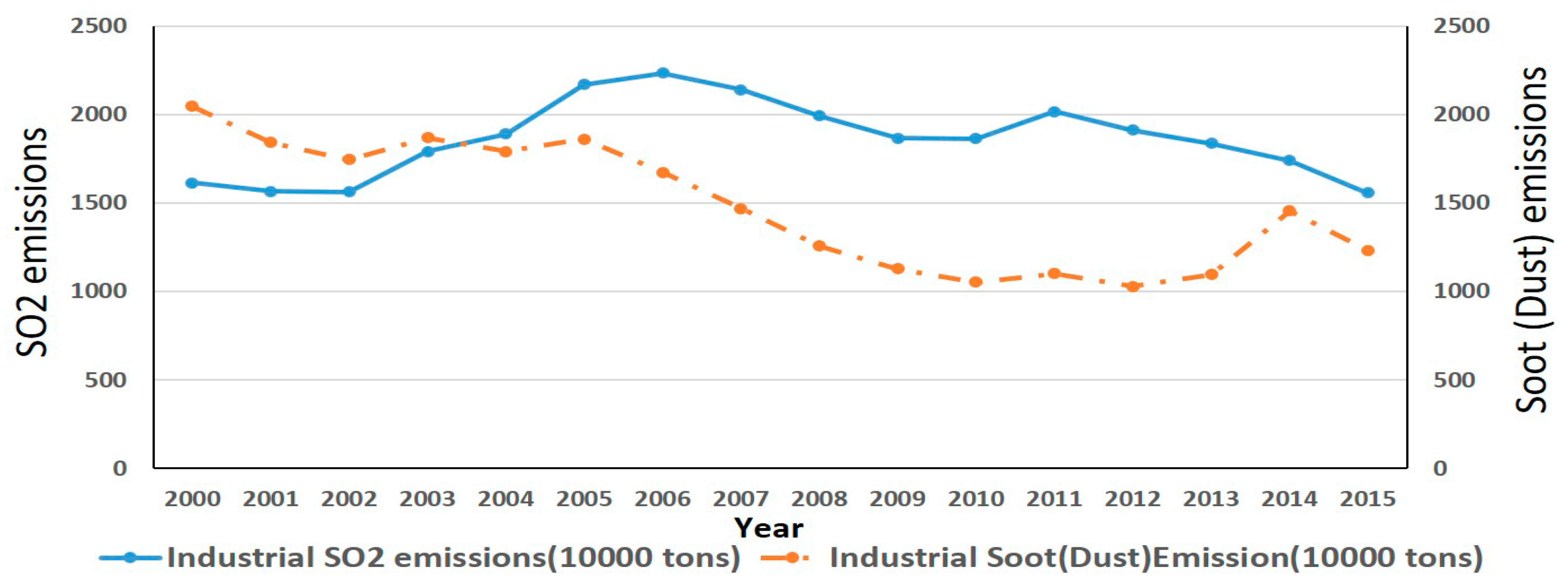
Emissions of industrial dust (soot) and SO₂ actually started to decline after 2005 (see Figure 1), although their absolute values are still high. Actually, the Chinese government had tried to reduce SO₂ emissions since 2007 in preparation for the 2008 Beijing Olympics. In Aug 2012, targeted energy conservation and emission reductions were proposed as part of the Chinese government’s 12th Five-year Plan (2011–2015). The Air Pollution Prevention and Control Action Plan issued by the State Council in 2013 aimed at reducing air pollution with specific targets. For example, by 2017, the urban concentration of inhalable particles should decrease by 10% compared with 2012 levels. The coexistence of rapid national economic growth and improved environmental conditions shows that Chinese environmental regulations and improved energy efficiency have played certain roles in this process.

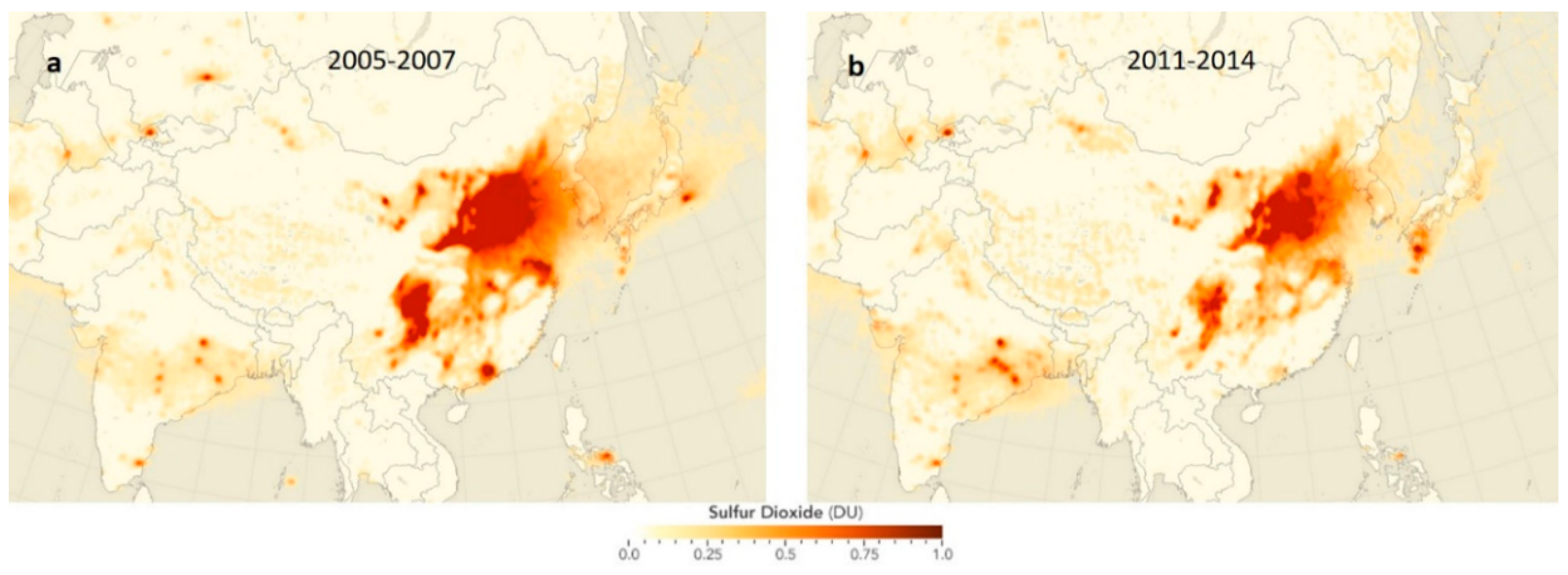
Foreign observational data also confirms declining SO₂ emissions in China (see Figure 2). The reduction of SO₂ is significant (about a 60% reduction from 2012 to 2015), although SO₂ levels in China remain the highest in the world [37,38]. This change shows that Chinese environmental regulation policies aiming at improving air quality have functioned well.

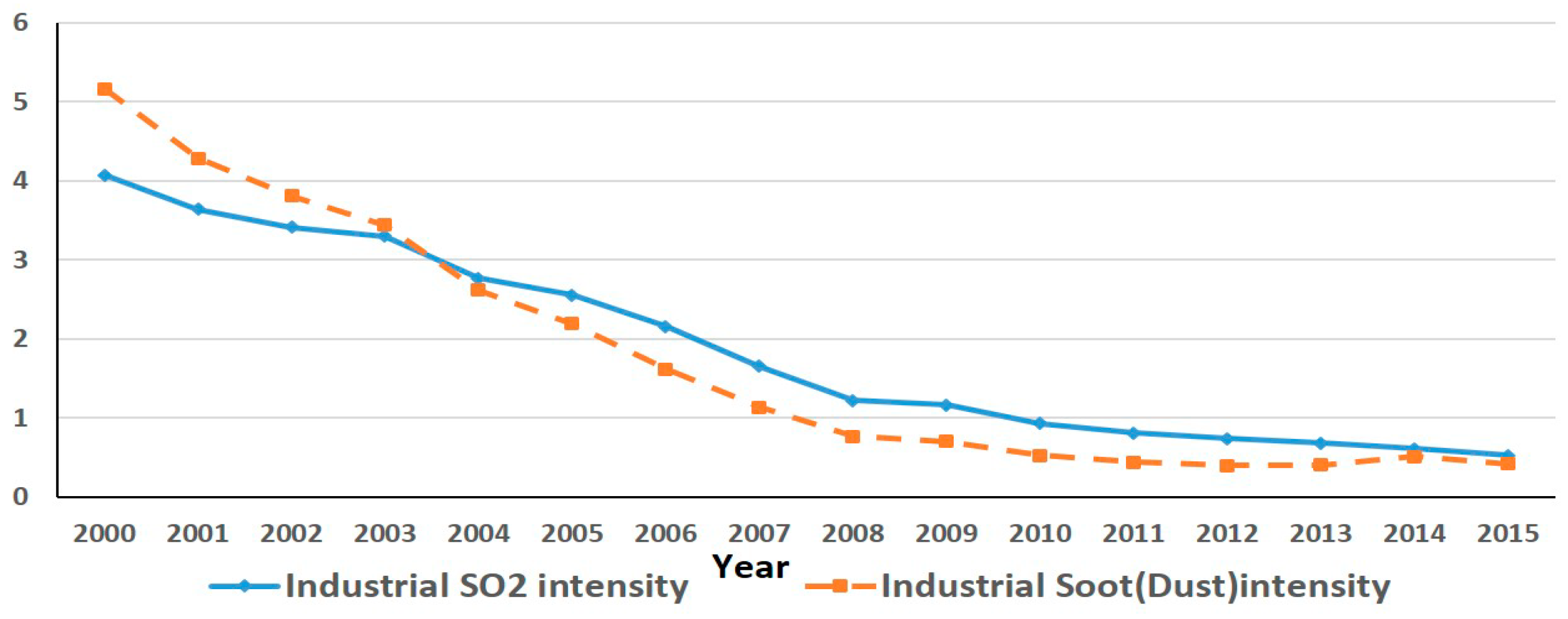
Apart from the decrease in absolute value, the change in relative level also indicates a similar trend in environmental regulations. This study combines pollution emissions with economic indexes to illustrate the pollution situation (see Figure 3), it’s clear that both intensities have been falling during the period, which further confirms the previous statements.

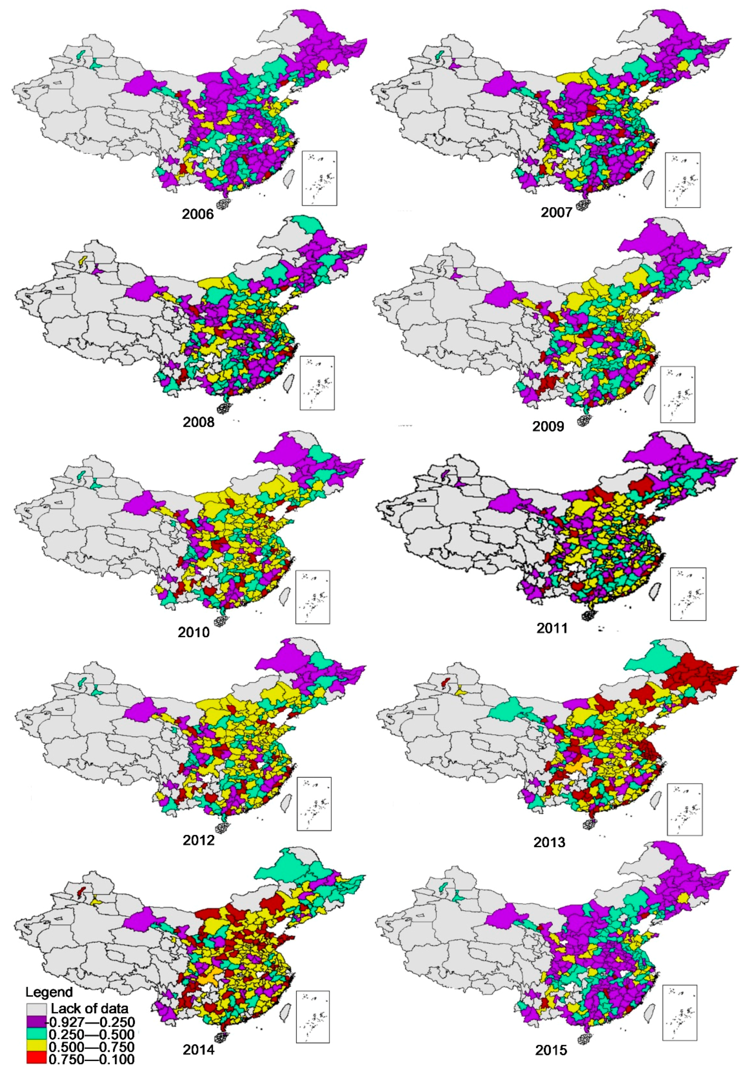
To examine specific changes in the intensity of environmental regulations, we plot the intensity over time for each pollutant (see Figure 4). The figure reveals that environmental regulations have been more stringent since 1990s. Then, what is the price for achieving this? Is the impact of environmental regulations on employment positive or negative in China?

3.2. The U-Shaped Relationship between Environmental Regulations and Employment

In the context of increasing intensity of environmental regulations, the economic growth pattern cannot adapt to it in the short term due to the development inertia, which eventually leads to a drop in the employment absorption capacity. According to the statistical data of China’s Ministry of Human Resources and Social Security in 2016, 13.14 million new jobs in urban areas were created. This is an increase of approximately 0.15 percent year-on-year, and the fourth straight year of remaining over 13 million. At the same time, there were approximately 15 million new unemployed youth who all need jobs, which indicates that the employment gap is large, especially considering those who cannot find a job over the years. In fact, urban registered unemployment in China hit 9 million in 2010. The unemployment rate has held at approximately 4 percent since then. Since Chinese unemployment registration system is deficient, a large gap exists between the registration and the actual condition.

In addition to the quantity contradiction, structural contradiction also affects the job market, which often manifests as more new jobs are created without enough qualified employees accompanied by the upgrade of the industrial structure. Therefore, it is necessary to account for the influence on the job market exerted by the government’s environmental regulations when formulating the policies. We cannot achieved this without a detailed understanding of the complex linkages between environmental regulations and the job market.

Previous researches have addressed the connection between environmental regulations and economy-wide employment. Since worker-level analyses are rare, this paper evaluates the effects of the regulations on worker-level employment. This theoretical model builds on the works of Cahuc (2004) [32] and Cole (2008) [23], in which pollution emissions were regarded as one production factor, and its price can be represented by environmental regulations. When environmental regulations become more stringent, the pollution costs of enterprises will be higher. This signal leads to a series of adjustments in production modes and employment. Based on this assumption, we build the partial equilibrium production model. This model supposes that: First, an enterprise has N kinds of production factors, including labor inputs, pollution inputs, and other inputs (like capital, technology etc. all represented by “other” for simplicity). Second, the intensity of regulations equals the pollution costs. Third, polluting enterprises will be regulated by the government through levying taxes, on carbon emissions or other polluting activities according to discharge standards. These punishments will directly increase the pollution costs. In other words, enterprises will choose the optimal combination of production factors in a given level of output that is determined by profit maximization. For simplicity, take a Cobb–Douglas production function to describe the enterprise’s production activities.

$$y_0=W^a{L}_0^{\beta }{T}^{\gamma },0<\alpha ,\beta ,\gamma <1$$

(1)

where $y_0$ denotes the output of the polluting enterprise, W denotes the pollution input, $L_0$ denotes the labor input, and T represents all other inputs. α, β, and γ are the pollution-elasticity, labor-elasticity and other factors’ elasticity, respectively ($0<\alpha ,\beta ,\gamma <1$). Enterprises select the level of W to maximize profit r:

$$MAX\left(r\right)=P{W}^a{L}_0^{\beta }{T}^{\gamma }-CW-V_0{L}_0-QT$$

(2)

where P denotes the price of products made by enterprises, $V_0$ represents the price of labor, Q denotes the price of other input factors, and C is the price of W. With the increasing intensity of environmental regulations, pollution costs will be higher, which increases C. There is a positive relationship between C and the intensity of environmental regulations. After the partial derivative of function MAX(r) with respect to the variable W, $L_0$ and T, we can get Equation (3) according to profit maximization.

$$L_0=\frac{\beta }{\alpha V_0}CW$$

(3)

Our measurement of the relationship between regulatory stringency and employment growth is based on the assumption that when environmental regulations are tightened, each enterprise faces a proportional rise in costs and will reduce its initial labor employment. It can be shown that:

$$\frac{d{L}_0}{dC}=\frac{\beta }{\alpha V_0}W\left(1-{\theta }_{WC}\right)$$

(4)

where ${\theta }_{WC}=-\left(\frac{C}{W}\right)\ast \left(\frac{dW}{dC}\right)$ represents the price elasticity of pollution inputs. Since C is already defined, it refers to the intensity of environmental regulations. ${\theta }_{WC}$ denotes the price elasticity of pollution inputs. When regulations are tightened, enterprises will reduce expenditures on pollution. Therefore, $dW/dC<0$. We add a minus sign in Equation (4) to make sure that ${\theta }_{WC}$ is non-negative. Equation (4) can be decomposed into two parts. First, $\beta W/\alpha V_0$ represents the employment change caused by the change in the relative price between $C$ and $L_0$, and we can call it the substitution effect. Second, $\left(\beta W/\alpha V_0\right){\theta }_{WC}$ represents the employment change caused by the change of enterprises’ production scales under the regulations, and we call this change the scale effect. These two effects have opposite signs.

The effect of $L_0$ on C is determined by ${\theta }_{WC}$. When ${\theta }_{WC}>$ 1, then $\beta W/\alpha V_0<\left(\beta W/\alpha V_0\right){\theta }_{WC}$ and the scale effect is bigger than the substitution effect. $d{L}_0/dC<0$, which implies that the effect of $L_0$ on C is negative. When ${\theta }_{WC}<1$, then $\beta W/\alpha V_0>\left(\beta W/\alpha V_0\right)$. $d{L}_0/dC>0$, and the effect is positive. Considering the economic meaning of ${\theta }_{WC}$, at the initial stage of environmental regulations, enterprises have to expand its pollution prevention investments to meet the regulatory standards. However, the quantity of this investment gradually diminishes, and the proportional decrease will be bigger than the increase in regulatory stringency. Therefore, ${\theta }_{WC}>1$. As regulations become more stringent, enterprises do not need to invest as much as the initial stage in pollution prevention. Since the room for decreasing pollution prevention investments is limited, the increasing degree of regulatory stringency will be bigger. Therefore, ${\theta }_{WC}<1$. The effect of a stringent environmental regulation policy can be summarized as follows. As environmental pollution intensity increases, ${\theta }_{WC}$ will change from $>$1 to $<$1 and $d{L}_0/dC<0$ will be replaced by $d{L}_0/dC>0$. In other words, the employment growth that accompanies the increase in environmental controls will be better after the deterioration in the initial stage.

After the analyses above, it could be found that there exists two effects of regulations on employment: the scale effect and the substitution effect. Increasing regulatory stringency will simultaneously create both, but the substitution effect is initially smaller than the scale effect, then bigger with the increase of investment in pollution prevention. That is to say, environmental regulations will increase an individual’s employment probability when the regulatory stringency reaches a given level. Therefore, there exists a “U” type relationship between environmental regulations and an individual’s employment probability.

Is the reality of China consistent with this? If the “U” relationship is true, are there any differences of the position of different regions of China in this U-shaped curve? Does industrial heterogeneity of the effect of regulations on an individual’s employment probability exist? These questions will be discussed in the empirical part of this paper.

3.3. Data Collection

The data about individual employment comes from the Chinese Household Income Project (CHIP) database [39]. This database covers income and expenditure information in 1988, 1995, 2002, 2007, 2008, and 2013. These are called CHIP1988, CHIP1995, CHIP2002, CHIP2007, CHIP2008, and CHIP2013, respectively. The CHIP survey consists of three parts: the Urban Household Survey, the Rural Household Survey, and the Migrant Household Survey. Considering that the survey did not cover rural-to-urban migrants before 2002 and the information absence, this paper chooses CHIP2007, CHIP2008, and CHIP2013 data as the data sources. The 2007 and 2008 surveys are also a part of the larger RUMiC (Rural-Urban Migrants in China) survey project. Both contain 5000 households in the migration sample, 8000 households in the rural sample, and 5000 households in the urban sample. The data comes from interviews with questionnaires designed by the project team.

For the surveys of urban local households and rural-urban migrant households, nine provinces were selected as the survey target in 2007 and 2008. They were Shanghai, Jiangsu, Zhejiang, and Guangdong from eastern China; Anhui, Henan, and Hubei from central China, and Chongqing and Sichuan from western China. The rural household survey also covered nine provinces. Differing from the urban and migrant’s surveys, Shanghai was excluded, while Hebei was included. The CHIP 2013 sample was selected by the systematic sampling method in the east, center and west. It contains 14 provinces. They are Beijing, Liaoning, Jiangsu, Shandong, and Guangdong from eastern China, Shanxi, Anhui, Henan, Hubei, Hunan, and Chongqing from central China, and Sichuan, Yunnan, and Gansu from western China. This provided a total of 126 cities, 234 counties, 18,948 households, and 64,777 individuals. In this, there are 7175 urban households, 11,013 rural households, and 760 migrant households. As CHIP focuses on the employment situation and the income and expenditure information, it has been widely accepted by scholars aiming at researching Chinese employment and income problems, like Bishop and Liu, 2008 [40]; Chen and Feng, 2011 [41]; Bishop et al., 2014 [42]; Gao et al., 2015 [43] and Li et al., 2017 [44]. That is also the primary reason that we choose CHIP as the input instead of others. Besides, CHIP also covers a survey of rural-to-urban migrants that makes it have the advantage of comparing different subsamples in the same topic then contributing to forming a comprehensive understanding of it. Other macro level data come from the China City Statistical Yearbook and the China Statistical Yearbook.

3.4. Econometric Model

An individual’s employment probability is defined as:

$$ur{e}_{ijt}={\alpha }_0+{\alpha }_{1}e{r}_{jt}+{\alpha }_{2}er{2}_{jt}+\beta X_{ijt}+{\delta }_j+{\mu }_t+{ϵ}_{ijt}$$

(5)

$$\begin{array}{l}{X}_{ijt}={\beta }_{0}lnsecondar{y}_{jt}+{\beta }_{1}lnope{n}_{jt}+{\beta }_{2}lnfa{i}_{jt}+{\beta }_{3}lnl{p}_{jt}\\ +{\beta }_{4}lnrgd{p}_{jt}+{\beta }_{5}lnf{e}_{jt}+{\beta }_{6}lninfr{a}_{jt}+{\beta }_{7}lnp{d}_{jt}\\ +{\beta }_{8}gende{r}_{ijt}+{\beta }_{9}ag{e}_{ijt}+{\beta }_{10}age{2}_{ijt}+{\beta }_{11}ma{r}_{ijt}\\ +{\beta }_{12}na{t}_{ijt}+{\beta }_{13}he{a}_{ijt}+{\beta }_{14}ed{u}_{ijt}\end{array}$$

(6)

where i denotes an individual, j denotes a city, t denotes the year, and $ur{e}_{ijt}$ (the dependent variable) is a dummy variable that denotes employment status (employed = 1, unemployed = 0). Those “not in the labor force” are eliminated from the sample data, which exclude retirees, students, homemakers, women who are pregnant or in maternity leave, and people on long-term sick leave. The age ranges are from 16 to 60 for men and 16 to 55 for women. $e{r}_{jt}$ represents the intensity of environmental regulations. Various methods can be used to measure it, including the emission density of different contaminants [45], the pollutant emissions volume per unit of output [46], a comprehensive index composed of multiple pollution indicators [47,48], a proxy index like per capita GDP [21,49] or cases of administrative penalty related to environmental protection [28,50]. The second method actually measures the pollution intensity without excluding the effect of technological and industrial factors. The third one is significantly affected by the weight of different indexes. Since per capita GDP, as an environmental regulation index, will be better among different countries than different regions of a country, the last one still has a lack of consensus. Xu and Song (2010) found that regions with higher average incomes does not necessarily have higher levels of environmental regulations [51]. Therefore, this study chooses the first method and adopts the emission density of sulfur dioxide (SO₂) in each city as the measurement index. Most studies establish a provincial index that measures the level of environmental regulations. Considering the imbalances in regional development, economic levels vary a lot within a province, the index used in this paper established at the city level will be more accurate and convincing.

$$e{r}_{jt}=\frac{\mathrm{Volume}\mathrm{of}\mathrm{Industrial}\mathrm{SO}2\mathrm{Removed}}{\mathrm{Volume}\mathrm{of}\mathrm{Industrial}\mathrm{SO}2\mathrm{Produced}}\ast 100\%$$

(7)

The data about industrial SO₂ emissions come from the China City Statistical Yearbook [52], $er{2}_{jt}$ is the quadratic term of the regulatory intensity. ${\delta }_j$ is an unobservable variable that is irrelevant to time. ${\mu }_t$ denotes the time dummy, and ${ϵ}_{ijt}$ is the error term. In Equation (6), $X_{ijt}$ represents the other factors that will affect $ur{e}_{ijt}$, including two categories: individual demographic characteristic and macro-level data. First, gender is represented by $gende{r}_{ijt}$ (man = 1, woman = 0). Age is represented by $ag{e}_{ijt}$ and its quadratic term $age{2}_{ijt}$ (unit is %). Nationality is represented by $na{t}_{ijt}$ (Han = 0, Minority = 1). $ma{r}_{ijt}$ denotes the marital status (single = 0, not single = 1). $ed{u}_{ijt}$ denotes years of formal education (excluding the number of years skipped or failed). Finally, $he{a}_{ijt}$ denotes one’s health condition (good = 1, not good = 0).

Next is the macro-level data. Fixed asset investments are denoted by $fa{i}_{jt}$, which is measured as the ratio between total investments in fixed assets in urban areas and GDP of each city. Fixed asset investments are one of the most important forces for economic growth and fostering job creation in China. The variable $f{e}_{jt}$ denotes government expenditure and is measured by the ratio between municipal expenditures and GDP. Due to the strong control of Chinese government over the economy, government expenditures are the main tool to achieve this, which then affects employment. Previous literatures have proven that, in the long run, an increase in public investment contributes to employment remarkably [53].

The variable $l{p}_{jt}$ denotes labor productivity measured by the ratio between annual gross output of all industrial enterprises above a designated size deflated by the GDP deflator (2000 as the base year) and the annual average number of workers in each city. Productivity growth has a positive impact on corporate profits but a significant negative effect on the labor demand per unit product. Therefore, labor productivity growth has a significant negative effect on employment growth [54].

The variable $rgd{p}_{jt}$ denotes the developmental level of the regional economy measured by the real GDP (2000 as the base year) of each city. A higher economic development level often means more jobs created.

The variable $secondar{y}_{jt}$ denotes the industrial structure measured by the share of second industrial output value to GDP. Different industries have different effects on employment [55]. A higher share of the second industry often means more jobs.

The variable $ope{n}_{jt}$ represents openness measured by the ratio between total actual FDI and the GDP of different cities. In an open economy, international investments will simultaneously create absorption and crowd-out effects. On one hand, foreign-capital enterprises will bring investments that will create more employment opportunities. On the other hand, it will diminish domestic investment and stimulate improved production efficiency, which have a negative effect on domestic employment. $infr{a}_{jt}$ and $p{d}_{jt}$ are used to measure regional infrastructure and urban population density. $infr{a}_{jt}$ represents the per capita area of paved roads in city. Since, enterprises are more likely to invest in a city with a higher infrastructure level, thereby more jobs will be created in these cities.

All macro-level data come from the China City Statistical Yearbook [52] and the China Statistical Yearbook [56]. To avoid the nonnormality and heteroscedasticity of variances, data of this level are logarithmically transformed.

In order to discuss the effects of regional and industrial heterogeneity, cities involved are divided into eastern, central, and western regions according to the standard released by the National Bureau of Statistics (NBS) of China in 2003. The industry classification standard comes from CHIP2013 that includes 20 Industries. The specific classification information and the matches between Chinese industries and US two-digit industries can be found in Table S1. The data sources and the meaning of indexes can be found in

Table 1. Data sources and brief descriptive statistics ¹.

Variables	Definition	Source	Obs.	Mean	SD	Max	Mini
$ur{e}_{ijt}$	Employment status	CHIP	67,364	0.991	0.094	1	0
$e{r}_{jt}$	Intensity of environmental regulations	China City Statistical Yearbook	267	0.462	0.267	0.998	0
$gende{r}_{ijt}$	Gender	CHIP	67,364	0.609	0.488	1	0
$ag{e}_{ijt}$	Age	CHIP	67,364	36.531	10.793	60	16
$ma{r}_{ijt}$	Marriage	CHIP	67,364	0.760	0.427	1	0
$ed{u}_{ijt}$	Education	CHIP	55,285	10.231	3.271	35	0
$na{t}_{ijt}$	Nationality	CHIP	67,364	0.019	0.135	1	0
$he{a}_{ijt}$	Health status	CHIP	67,364	0.984	0.125	1	0
$fa{i}_{jt}$	Fixed asset investments	China City Statistical Yearbook	271	0.635	0.252	2.026	0.120
$l{p}_{jt}$	Labor productivity	China City Statistical Yearbook	270	49.989	58.721	363.255	0.056
$rgd{p}_{jt}$	Municipal real GDP	China City Statistical Yearbook	272	1592.255	1927.201	11,731.700	122.851
$secondar{y}_{jt}$	Industrial structure	China Statistical Yearbook	250	0.495	0.092	0.746	0.217
$ope{n}_{jt}$	Openness	China City Statistical Yearbook	265	0.026	0.022	0.112	0.0001
$f{e}_{jt}$	Government expenditures	China Statistical Yearbook	271	0.150	0.082	0.701	0.058
$infr{a}_{jt}$	Infrastructure level	China City Statistical Yearbook	252	15.256	6.488	38.200	0.390
$p{d}_{jt}$	Population density	China Statistical Yearbook	271	558.131	344.082	2616.230	5.710

¹ The data source of summary statistics comes from author calculation, the year range covers 2007, 2008, and 2013. SD represents standard deviation.

.

Table 1 shows that most observations have a job, and their education is over junior middle school. Openness varies greatly across the sample, the smallest one is 0.25, 0.19, and 0.12 percent of the size of the largest ones in 2007, 2008, and 2013, respectively. Most individuals are married and of the Han nationality. We also find that China’s economic level varies across regions. The highest city’s real GDP is approximately 83.76, 78.73, and 75.77 times bigger than the lowest one in 2007, 2008, and 2013, respectively.

4. Results

4.1. General Results

As CHIP2007, CHIP2008, and CHIP2013 are used in this paper and merged into a pooled crossed-section regression data, and the dependent variable is a dummy variable. The model (Equation (5)) is estimated using the probit model and year and region dummies are included in all estimations. The general results could be found in Appendix A. The reported coefficients represent the marginal effect of variables at mean (

Table A1. Determinants of an individual’s probability of being employed.

Variable	Probit Estimation			Probit Estimation with One Year Lagged
	(1)	(2)	(3)	(4)	(5)	(6)
$e{r}_{jt}$	−0.0170 ***			−0.0196 ***
	(0.263)			(0.308)
$er{2}_{jt}$	0.0165 ***			0.0234 ***
	(0.254)			(0.342)
$er{b}_{jt}$		−0.0862 ***			−0.0415 **
		(1.378)			(0.890)
$erb{2}_{jt}$		0.0558 ***			0.0320 **
		(0.883)			(0.673)
$er{s}_{jt}$			−0.0050 ***			−0.0036 **
			(0.079)			(0.077)
$ers{2}_{jt}$			0.0003			0.0003
			(0.018)			(0.022)
$gende{r}_{ijt}$	0.0012	0.0012	0.0012	0.0012 *	0.0014 *	0.0014 *
	(0.035)	(0.035)	(0.035)	(0.035)	(0.035)	(0.035)
$ag{e}_{jt}$	0.00009	0.00007	0.0001	0.00012	0.00007	0.0001
	(0.013)	(0.013)	(0.013)	(0.014)	(0.014)	(0.014)
$age{2}_{jt}$	−0.00031	−0.00028	−0.0003	−0.00032	−0.00028	−0.0003
	(0.016)	(0.016)	(0.016)	(0.017)	(0.017)	(0.017)
$ma{r}_{ijt}$	0.0018	0.0018	0.0018	0.0016	0.0019	0.0018
	(0.060)	(0.060)	(0.060)	(0.061)	(0.061)	(0.061)
$na{t}_{ijt}$	−0.0059 ***	−0.0057 ***	−0.0057 ***	−0.0037 **	−0.0049 **	−0.0046 **
	(0.090)	(0.090)	(0.090)	(0.091)	(0.091)	(0.091)
$he{a}_{ijt}$	0.0084 ***	0.0085 ***	0.0084 ***	0.0076 ***	0.0089 ***	0.0090 ***
	(0.092)	(0.092)	(0.092)	(0.092)	(0.091)	(0.091)
$ed{u}_{ijt}$	0.0003 ***	0.0003 ***	0.0004 ***	0.0003 ***	0.0003 ***	0.0004 ***
	(0.005)	(0.005)	(0.005)	(0.005)	(0.005)	(0.005)
$lnsecondar{y}_{jt}$	0.0015	0.0013	0.0034	0.0047 **	0.0037	0.0072 ***
	(0.101)	(0.103)	(0.109)	(0.116)	(0.117)	(0.116)
$lnope{n}_{jt}$	0.0005	0.0003	0.0001	−0.00001	−0.0001	−0.0002
	(0.022)	(0.021)	(0.021)	(0.021)	(0.021)	(0.022)
$lnfa{i}_{jt}$	−0.0025 *	−0.0023 *	−0.0022	−0.0015	−0.0011	−0.0018
	(0.061)	(0.060)	(0.063)	(0.070)	(0.069)	(0.071)
$lnl{p}_{jt}$	0.0000	0.0002	−0.0002	0.0006	0.0006	0.0006
	(0.016)	(0.016)	(0.016)	(0.019)	(0.019)	(0.019)
$lnrgd{p}_{jt}$	0.0016 **	0.0013 **	0.0004	0.0008	0.0004	−0.0001
	(0.030)	(0.031)	(0.030)	(0.038)	(0.037)	(0.037)
$lnf{e}_{jt}$	0.0018	0.0022	0.0028 *	−0.0004	−0.0019	−0.0001
	(0.071)	(0.072)	(0.075)	(0.098)	(0.095)	(0.100)
$lninfr{a}_{jt}$	0.0011	0.0016 **	0.0008	0.0027 ***	0.0033 ***	0.0027 ***
	(0.036)	(0.034)	(0.039)	(0.041)	(0.044)	(0.042)
$lnp{d}_{jt}$	−0.0005	−0.0002	−0.0010	0.0011 *	0.0001	0.0003
	(0.025)	(0.025)	(0.030)	(0.035)	(0.023)	(0.039)
mc	Control	Control	Control	Control	Control	Control
pc	Control	Control	Control	Control	Control	Control
2008 year dummy	Control	Control	Control	Control	Control	Control
2013 year dummy	Control	Control	Control	Control	Control	Control
Constant	1.610 **	2.823 ***	1.695 **	0.384	1.616 **	0.669
	(0.707)	(0.840)	(0.707)	(0.742)	(0.772)	(0.746)
pseudo R2	0.039	0.038	0.043	0.047	0.042	0.046
Obs.	54298	54298	54298	51502	51785	51432

Note: Determinants of an individual’s probability of being employed. Source: own estimations from survey data. The numbers in parentheses are robust standard errors. * significant at 10% level; ** significant at 5% level; *** significant at 1% level. Mc represents municipality dummy (Yes = 1, No = 0), pc represents provincial capital dummy (Yes = 1, No = 0), which is the same to other estimations. The dependent variable is $ur{e}_{ijt}$. Regression models are estimated using Equation (5).

). Column (1) reports that regulatory intensity measured by the proportion of industrial SO₂ removed ($e{r}_{jt}$) has a significantly negative effect on an individual’s employment probability at the 1% level. The coefficient of the quadratic term of the regulation intensity ($er{2}_{jt}$) is significantly positive at the 1% level too, which proves that the U-shaped curve exists between environmental regulations and an individual’s employment probability. We can find the knee point of this U-shaped curve, which is approximately 0.515 according to the coefficients $e{r}_{jt}$ and $er{2}_{jt}$. Compared with the average regional regulatory intensity of 2013, we find that the average intensity of environmental regulations in most cities are already in the upward phase of the U-shaped curve. From a regional perspective, those still in the downward phase were mainly located in western China. (The precise results are shown in

Table 2. Regional intensity of environmental regulation statistics in 2013.

$\mathit{e}{\mathit{r}}_{\mathit{j}\mathit{t}}$	Obs.	Mean	SD	Max	Mini 1
National	278	0.5943	0.2913	0.9983	−0.9267
Eastern Region	96	0.6569	0.2222	0.9983	0
Central Region	98	0.6008	0.3185	0.9871	−0.7484
Western Region	84	0.5150	0.3118	0.9815	−0.9267

¹ The minimum value appears negative, which means that the volume of SO₂ produced is less than the volume removed in some cities. The reason leading to this strange situation is that some industrial enterprises store or conceal part of the SO₂ produced to complete the assessment of local governments.

). Table A1 also shows that men have an advantage over women in finding a job, although the gap is narrow. A healthy body also significantly improves the probability of being employed. One more year of education increases the probability of being employed by 0.03%. The coefficients of age and its quadratic term suggest that the relationship between a worker’s age and the probability of being employed is an inverted U-shape. The coefficients of $lnsecondar{y}_{jt}$, $lnope{n}_{jt}$, $lnf{e}_{jt}$, and $lnrgd{p}_{jt}$ (respectively represent the logarithm of $secondar{y}_{jt}$, $ope{n}_{jt}$, $f{e}_{jt}$ and $rgd{p}_{jt}$) are positive, which are consistent with our expectations. The result shows that improved infrastructure is a favorable factor for increasing employment probability. However, the coefficient of $lnfa{i}_{jt}$ is not consistent with our prior expectations, which indicates that the effect of fixed assets investments on employment growth varies among different periods.

Considering that environmental regulations usually cannot have an immediate influence upon employment, this lag may underestimates the effect of environmental regulations. To avoid the interference, we use all macro independent variables with one year lagged to replace the original ones. The regression results are shown in column (4) of Table A1, which proves that the “U” type relationship still exists.

4.2. Robustness Check

Endogeneity is a potential problem for some of our regulation indexes. For example, the regional unemployment rate could be endogenously determined by pollution intensity rather than the other way around. It could be argued that those cities with high economic activities that attract workers through higher salaries usually have poorer environmental quality and high environmental regulations [57]. Endogeneity concerns should be examined in the results. We choose a substitution index as the instrumental variable of environmental regulation. The proportion of industrial soot removed ($er{b}_{jt}$) is measured by the ratio between the volume of industrial soot removed and the volume of industrial soot produced:

$$er{b}_{jt}=\frac{\mathrm{Volume}\mathrm{of}\mathrm{Industrial}\mathrm{Soot}\mathrm{Removed}}{\mathrm{Volume}\mathrm{of}\mathrm{Industrial}\mathrm{Soot}\mathrm{Produced}}\ast 100\%$$

(8)

Column (2) (Table A1) reports the results of the probit model with $er{b}_{jt}$ as the regulatory intensity. Column (5) (Table A1) reports the probit estimation with one year lagged based on CHIP2007, CHIP2008, and CHIP2013 with this index. They all show that there is a “U” type relationship between environmental regulations and an individual’s probability of being employed. Therefore, our conclusion is robust.

The index selection above is not, to a degree, a systematic reflection of environmental regulations. Therefore, following Wang and Liu (2014) [58], we set a comprehensive measurement index. Specifically, the linear weighted sum method is used to set a comprehensive index of environmental regulation intensity ($er{s}_{jt}$) based on the proportion of industrial SO₂ and soot removed. First, we standardize $e{r}_{jt}$ and $er{b}_{jt}$:

$$p{r}_{jk}^s=\left[p{r}_{jk}-\min \left(p{r}_k\right)\right]/\left[\max \left(p{r}_k\right)-\min \left(p{r}_k\right)\right]$$

(9)

where $p{r}_{jk}$ represents the proportion of pollutant k removed in city j. $\max \left(p{r}_k\right)$ and $\min \left(p{r}_k\right)$ represent the maximum and minimum of $p{r}_{jk}$, respectively. $p{r}_{jk}^s$ denotes the standardized value of $p{r}_{jk}$. Second, as the share of industrial SO₂ and soot emission varies in different cities, the emission levels of different pollutants are different, even within a city. It is necessary to endow different weights for each pollution emission index of each city, so as to get a precise description of the change of regulatory intensity of each city. Here, we set an adjustment coefficient ($A_{jk}$) as the weight:

$$A_{jk}=\frac{p{e}_{jk}}{{{\displaystyle \sum }}_{j}p{e}_{jk}}/\frac{gd{p}_j}{{{\displaystyle \sum }}_{j}gd{p}_j}$$

(10)

This coefficient means that the ratio between the proportion of the emission volume of pollutant k to the total emissions in China and the rate of GDP of city j to national GDP. The intensity of environmental regulations of one city will be stronger than others with the same $e{r}_t$ or $er{b}_t$ if the emission volume of SO₂ or soot is relatively larger when we add this coefficient into our indexes. Since the proportion of removed SO₂ or soot is an absolute value and GDP reflects the scale and level of economic development of one city, the combination of both can more objectively reflect the regulatory intensity of different cities. Therefore, $er{s}_{jt}$ can be expressed as:

$$er{s}_{jt}=\left({{\displaystyle \sum }}_{k=1}^2{A}_{jk}p{r}_{jk}^s\right)/2$$

(11)

Column (3) and (6) in Table A1 report the results of the probit model with $er{s}_{jt}$ as the regulatory intensity. Column (6) reports results of the regression variables with one year lagged. They all show that there still exists a “U” type relationship between environmental regulations and an individual’s probability of being employed. It further confirms the robustness of our conclusion.

4.3. Heterogeneity Checks

4.3.1. Is There Heterogeneity in the Regulatory Effects across Regions?

This subsection explores whether the regulatory effects vary across different regions. As the level of economic development is highly imbalanced among the three regions, it is necessary to consider local situations and the position of different cities is in a downward or upward phase of the U-shaped curve. It (Table 2) presents the differences in regional regulatory intensity in 2013.

Table 2 suggests that the eastern and central regions are already in the upward phase of the U-shaped curve (value of the knee point approximately 0.515), but the western is near the knee point. The double dividend effect of the positive relationship between productivity growth and employment growth still does not appear in the western area, which is coincident with Lu (2011) [59]. Therefore, the tradeoff between employment and the environment should be weighed carefully in different regions.

According to Li’s classification method (2016) of high-pollution industries, the value of high-pollution industrial production is relatively higher. It could be found that the value of industrial production of pollution-intensive industries (including coal mining and dressing, ferrous metals mining and dressing, nonferrous metals mining and dressing, farm products processing, textile industry, paper making and paper products, petroleum processing, coking and nuclear fuel processing, raw chemical materials and chemical products, chemical fibers, nonmetal mineral products, smelting and pressing of ferrous metals, smelting and pressing of non-ferrous metals and electric power, heat power production and supply) in the eastern region is approximately 2.8 and 5.3 times greater than the central and western regions, respectively, during 2007–2013 [30]. Therefore, the average regulation in the eastern region is more stringent. However, the standard deviation is larger in the central region, which indicates a vast internal diversity within the central region, and this difference between different regions is not accidental. When we use different colors to represent the values of $e{r}_{jt}$ of each city in the map (Figure 5), it shows that the difference in the regulatory intensity index among central cities is larger, and the overall intensity of environmental regulations increased from 2006 to 2014. During this time, we can also find that the environmental regulations of eastern cities are more stringent.

Table A2. Heterogeneity in the regulatory effects across regions.

Variable	Eastern Region	Central Region	Western Region
$e{r}_{jt}$	−0.0188 **	−0.0120	0.0124
	(0.552)	(0.461)	(0.866)
$er{2}_{jt}$	0.0153 **	0.0183	−0.0043
	(0.452)	(0.546)	(0.888)
$gende{r}_{ijt}$	0.0013	0.0015	0.0002
	(0.055)	(0.054)	(0.086)
$ag{e}_{jt}$	−0.00008	0.00011	0.00045
	(0.022)	(0.021)	(0.028)
$age{2}_{jt}$	0.0001	−0.0005	−0.0009
	(0.027)	(0.025)	(0.035)
$ma{r}_{ijt}$	0.0007	0.0014	0.0042 *
	(0.093)	(0.097)	(0.133)
$na{t}_{ijt}$	−0.0036 *	−0.0077 *	−0.0055
	(0.137)	(0.144)	(0.266)
$he{a}_{ijt}$	0.0090 ***	0.0089 **	0.0037
	(0.149)	(0.142)	(0.215)
$ed{u}_{ijt}$	0.0004 ***	0.0003	0.0003
	(0.009)	(0.007)	(0.012)
$lnsecondar{y}_{jt}$	−0.0031	−0.0031	−0.0076
	(0.165)	(0.202)	(0.612)
$lnope{n}_{jt}$	−0.0001	0.0020 **	0.0020
	(0.047)	(0.035)	(0.076)
$lnfa{i}_{jt}$	0.0032 **	0.0019	−0.0016
	(0.098)	(0.143)	(0.209)
$lnl{p}_{jt}$	−0.00008	0.0029 **	−0.0015 *
	(0.024)	(0.045)	(0.051)
$lnrgd{p}_{jt}$	0.0003	0.0011	−0.0070 **
	(0.059)	(0.064)	(0.162)
$lnf{e}_{jt}$	−0.0003	−0.0141 **	−0.0064 *
	(0.113)	(0.200)	(0.212)
$lninfr{a}_{jt}$	0.0003	0.0121 ***	−0.0033
	(0.058)	(0.091)	(0.256)
$lnp{d}_{jt}$	0.0031 ***	0.0018	−0.0013
	(0.069)	(0.065)	(0.098)
mc	Control	Control	Control
pc	Control	Control	Control
2008 year dummy	Control	Control	Control
2013 year dummy	Control	Control	Control
Constant	0.720	1.544	8.642 **
	(1.241)	(1.170)	(4.067)
pseudo R2	0.058	0.045	0.061
Obs.	26602	18025	9671

Note: Heterogeneity in the regulatory effects across regions. Source: own estimations from survey data. The numbers in parentheses are robust standard errors. * significant at 10% level; ** significant at 5% level; *** significant at 1% level. The dependent variable is $ur{e}_{ijt}$. Regression models are estimated using Equation (5).

(Appendix A) displays the principal results of the effects of environmental regulations on an individual’s probability of being employed across regions.

The results suggest that the “U” type relationship between the intensity of environmental regulations and an individual’s probability of being employed exist in the eastern and central regions, although the estimation of the central region is not significant. For the western region, the employment probability follows an insignificant inverted U-shaped pattern related to the intensity of environmental regulations.

This result indirectly reflects the imbalance in regional economic development. It can be stated that regardless of per capita added value of the industry or the proportion of employment, the eastern region is higher than the central and western regions. Moreover, the government executive abilities in the eastern region are higher. New regulatory policies can be effectively carried out, whereas economic growth trumps green priorities in the western and central regions. Therefore, those policies will not function well or will totally lose their regulatory functions. The probability of being employed in the eastern region is more sensitive to the changes in regulatory intensity.

With respect to the western region, the industrial structure is not diverse enough. The proportion of high-pollution, high energy-consuming industries is relatively lower. Therefore, the pollution intensity is weaker. As environmental regulations become increasingly stringent, more eastern and central enterprises tend to transfer their factories to the west, which may lead to a “Pollution Haven”. However, when the intensity of regulations meets a given threshold level, their cost savings due to weaker regulatory intensity cannot cover the extra expenses of production in the west. Then, they will relocate to eastern or central cities, resulting in a decrease of employment opportunities. The estimation (Table A2) shows that the value of the knee point of the western region is approximately 1.45, far above the average regulatory intensity. Thus more stringent regulations will benefit the employment of the western cities.

The difference of environmental regulatory intensity among cities poses new challenges to the equilibrium development among regions. More low-value-added and traditional industries will be forced to transfer to the western region when they cannot adjust to the regulatory intensity in the eastern and middle regions. Divergent regulatory policies aimed at different regional situations should be adopted to obtain a double dividend effect. Meanwhile, the local government should form a long-term perspective about the effect of environmental regulations on employment. This trade-off between employment and environmental protection must be given great emphasis.

4.3.2. Is There Heterogeneity in the Regulatory Effects across Industries?

Do the regulatory effects vary by industry due to the differences in the utilization of resources, pollution emissions, technological level, bargaining power, and others among industries? This subsection explores this heterogeneity in reference to the industrial classification standard made by CHIP2013. As the estimated result of the probit model is in accordance with the Linear Probability Model (LPM), and for the convenience of the comparison of different coefficients and identifying the average treatment effect [60], we use the LPM to conduct the regression analysis of these 19 respective industries (The sample from the industry of International Organizations is so small that we eliminate it from our model.). Each row in

Table A3. Heterogeneity in the regulatory effects across industries.

Industry & Code	$\mathit{e}{\mathit{r}}_{\mathit{j}\mathit{t}}$	$\mathit{e}\mathit{r}{\mathbf{2}}_{\mathit{j}\mathit{t}}$	R2	Obs.	Industry & Code	$\mathit{e}{\mathit{r}}_{\mathit{j}\mathit{t}}$	$\mathit{e}\mathit{r}{\mathbf{2}}_{\mathit{j}\mathit{t}}$	R2	Obs.
01. Agriculture, forestry, animal production and hunting, fishing	−0.0325	0.0524	0.026	1007	11. Real estate	0.1202	−0.1224	0.038	863
	(−0.066)	−0.063				(−0.105)	(−0.122)
02. Mining and quarrying	0.0148	0.0242	0.025	766	12. Leasing and business services	−0.0172	0.0104	0.012	1182
	(−0.093)	(−0.078)				(−0.065)	(−0.064)
03. Manufacturing	−0.0157	0.0191 **	0.004	12937	13. Scientific research, technical services	−0.0309	0.0327	0.055	771
	(−0.010)	(−0.009)				(−0.047)	(−0.054)
04. Production and distribution of electricity heating power, gas and water	0.0338	−0.0223	0.026	993	14. Management of water conservancy, environment and public facilities	0.138	−0.2066 *	0.081	399
	(−0.067)	(−0.055)				(−0.086)	(−0.121)
05. Construction	−0.0382*	0.0108	0.019	5798	15. Household services, repair and other services	−0.0232	0.0223	0.011	5348
	(−0.021)	(−0.021)				(−0.031)	(−0.029)
06. Transportation, warehousing and post	−0.0215	0.0274	0.013	3721	16. Education	−0.0646*	0.0505	0.019	1708
	(−0.029)	(−0.028)				(−0.036)	(−0.037)
07. Information transmission, computer services and software	−0.0062	0.0059	0.024	1238	17. Health, social work	0.0479	−0.0454	0.01	1404
	(−0.014)	(−0.023)				(−0.036)	(−0.036)
08. Wholesale and retail trade	−0.0253	0.0415 *	0.01	7813	18. Culture, sports and entertainment	−0.0231	0.0176	0.029	729
	(−0.022)	(−0.022)				(−0.048)	(−0.042)
09. Hotels and catering services	−0.0428	0.0422	0.011	4089	19. Public management social security and social organization	−0.006	0.0021	0.016	2606
	(−0.030)	(−0.032)				(−0.007)	(−0.014)
10. Finance and Insurance	0.0504	−0.0532	0.029	913
	(−0.050)	(−0.065)

Note: Heterogeneity in the regulatory effects across industries. Source: own estimations from survey data. The numbers in parentheses are standard errors. * significant at 10% level; ** significant at 5% level; *** significant at 1% level. The dependent variable is $ur{e}_{ijt}$. Regression models are estimated using Equation (5). The results of other control variables are not presented here because of space considerations.

(Appendix A) pertains to an industry. This allows us to compare the differences of the regulatory effects in each of the relevant industries.

The “U” type relationship between environmental regulations and an individual’s probability of being employed still exists in most industries. The effects of regulations are particularly significant in industries like manufacturing, the wholesale and retail trade, construction, the management of water conservancy, environmental and public facilities, and education. However, the employment probability follows an inverted U-shaped pattern related to environmental regulations in service industries like finance and insurance, real estate, the management of water conservancy, environmental and public facilities, health, and social work. This is consistent with our expectation. As most service industries do not produce emissions and are expanding in China, at the same time, most workers are likely to transfer to these industries from those strongly affected by environmental regulations. There exists positive short run effects of environmental regulations on these service industries until the point where the level of environmental regulations meet the knee point of each industry. While the results also show that with the increase of environmental regulation intensity, an individual’s probability of being employed in mining and quarrying industry will increase instead of a U-shaped pattern. The reason may be that traditional pollution-intensive industries are regarded as a major regulating object during the early stages of pollution regulation, which in turn contributes to them becoming pioneer in industrial upgrading. It can be found that China’s environmental protection laws and regulations were aimed at industries like electricity, coal, steel, cement, non-ferrous metals, coke, and other pollution-intensive industries during the early stages, such as Guidance Directory of Industrial Restructuring of 2005, 2007, and 2011 and The Temporary Provision Rules for Promotion of Adjustment of Industrial Structure which was deliberated on and passed by the executive meeting of the State Council in March 2008, etc. On one hand, those regulations placed great stress on the involved industries’ sustainability, on the other hand, they also made them gain first-mover advantage in industrial transformation and upgrading, the elasticity coefficient of employment in this industry to the change of environmental regulations is relatively smaller, and even positive under certain conditions. When these 19 industries are divided into three categories according to the “Regulation on Classification of Three Sectors (GB/T 4754—2011)” promulgated by NBS in 2012 (the specific classification details can be found in Table S2), the results (

Table 3. Heterogeneity in the regulatory effects by three strata of industry ^1,2.

Variable	Primary Industry	Secondary Industry	Tertiary Industry
$e{r}_{jt}$	−0.01836	−0.01491 *	−0.01489 *
	(1.513)	(0.437)	(0.350)
$er{2}_{jt}$	0.03540	0.01302 *	0.01551 **
	(1.590)	(0.405)	(0.346)
mc	Control	Control	Control
pc	Control	Control	Control
2008 year dummy	Control	Control	Control
2013 year dummy	Control	Control	Control
Constant	−6.7662	1.1003	1.9887 **
	(4.536)	(1.353)	(0.875)
pseudo R2	0.137	0.059	0.036
Obs.	1007	20,494	32,797

¹ The numbers in parentheses are robust standard errors. * significant at 10% level; ** significant at 5% level; *** significant at 1% level. ² The reported results represent the marginal effect of variables, which are estimated by the probit model and other control variables are not presented here because of space considerations.

) support the existence of a “U” type relationship in three categories, but it is not significant in primary industry. Since primary industry produces relatively little pollution, the impacts of environmental regulations on employment in these industries are quite limited. Therefore, after removing samples related to primary industry, the significant “U” type relationship in secondary and tertiary industry further confirms our conclusion.

The heterogeneity among industries illustrates the mobility of labor between industries. Generally, industries such as the production and distribution of electricity heating power, gas and water, the management of water conservancy, environmental and public facilities, health, and social work are controlled by governmental organizations or public institutions that are in a position of market dominance to some degree. Their anti-risk capacity helps to free them from policy shocks, and the effects of regulations are limited. In addition, these industries have a close relationship with the government, and their bargaining power enables them to negotiate the regulatory conditions. All these factors make them more attractive to workers due to more steady jobs than those in other industries.

While competitive industries like manufacturing, construction, wholesale, and retail trade are exposed to the impacts of regulations, in the short run, the increasing regulatory stringency will raise the operating costs of these industries. This will in turn downsize their production scale or force them to exit the market. Workers in these industries will transfer to others that face less stringent regulations. Therefore, more labor flows to service industries, government organizations, and public institutions. In the long term, when various traditional industries finish upgrading the industrial structure and adjust to the limits of regulations, emerging industries transformed from the traditional ones will create more new jobs, and a backflow of labor will occur in these industries. That is why we can see the inverted U-shaped curve between the intensity of environmental regulations and the probability of being employed in finance and insurance, real estate, and other service industries, governmental organizations, and public institutions. Most rural migrant workers engage in manufacturing and construction [61], in which the effect of environmental regulations on employment is very significant. It is crucial to analyze the heterogeneity in the regulatory effects across groups of labor, especially rural migrant workers.

4.3.3. Is There Heterogeneity in the Regulatory Effects across Hukou of Labor?

The household registration system, the separated labor market resulting from the urban-rural dual structure, and the differences of social insurance, information acquisition, and employment opportunities for different hukou lead to a noticeable gap in available job resources, career stability, and anti-risk capacity. Usually, urban-hukou employees are relatively highly skilled and possess employment security and longer average years of education, which strengthen their anti-risk capacities. Therefore, the effect of regulations is weaker on them compared with rural-hukou employees whose jobs are often not stable. The risk of non-agricultural employment is principally relieved by the rationality of farmer households. Owing to constraints imposed by the urban-rural dual structure and the land equalization system as the basic relationships of property, the endogenous rationality of agricultural households and rural communities can internalize external risks. This means that hundreds of millions of rural migrant workers undertake this risk with risk-free assets (land distributed equally through non-market ways in each family-unit) [62].

Table 4. Heterogeneity in the regulatory effects across different hukous of labor ^1,2.

Variable	Rural Male	Rural Female	Migrant Male	Migrant Female	Urban Male	Urban Female
	(1)	(2)	(3)	(4)	(5)	(6)
$e{r}_{jt}$	−0.0042	−0.0031	−0.0002	−0.0017 ***	−0.0406 ***	−0.0636 ***
	(0.471)	(0.579)	(3.387)	(4.830)	(0.578)	(0.863)
$er{2}_{jt}$	0.0032	0.0042	0.00007	0.0016 ***	0.0418 ***	0.0586 ***
	(0.455)	(0.520)	(2.966)	(5.359)	(0.579)	(0.868)
mc	Control	Control	Control	Control	Control	Control
pc	Control	Control	Control	Control	Control	Control
2008 year dummy	Control	Control	Control	Control	Control	Control
2013 year dummy	Control	Control	Control	Control	Control	Control
Constant	3.8947 **	1.6625	2.3954	−1.6354	−2.2718	0.1423
	(1.816)	(1.987)	(6.839)	(7.496)	(1.539)	(1.891)
pseudo R2	0.084	0.050	0.290	0.368	0.067	0.053
Obs.	13,595	8242	7037	4616	12,064	8555

¹ The numbers in parentheses are robust standard errors. * significant at 10% level; ** significant at 5% level; *** significant at 1% level. ² The reported results represent the marginal effect of variables which are estimated by the probit model. Other control variables are not presented here because of space considerations.

provides estimated results of different hukous of labor using Equation (5). Columns (1)–(2) and (3)–(4) display the employment probability changes caused by different regulatory intensities with farmers and rural migrant workers. Those coefficients indicate that the “U” type relationship between environmental regulations and an individual’s employment probability still exist. Columns (5)–(6) present the results of urban workers, which shows a significant “U” type relationship.

Specifically, the effects of environmental regulations on the employment probability of rural workers, regardless of gender, are not significant. It can be explained that most rural workers occupy primary industries that do not produce SO₂, soot, dust, or other pollutants. Therefore, increasing intensity of environmental regulations will have little influence on the employment of this industry. However, the results indicate that migrant female workers experience a stronger impact from environmental regulations than males. This proves that, to a certain extent, gender inequality still exists in the job market. Moreover, most migrant workers are temporary workers that do not have labor contracts with enterprises. According to the data obtained from annual Investigation Report on Rural Migrant Workers in China [61], the proportion of migrant workers don’t have a labor contract with employers is 56.1%, 58.7%, 62%, 63.8%, and 64.9% in 2012, 2013, 2014, 2015, and 2016, respectively, which shows an upward tendency. When environmental regulations become more stringent, employers tend to improve the production technology or downsize their factories to save costs, which all have negative effects on employment. Due to their disadvantages in labor productivity and social status, migrant female workers are more likely to be fired. For urban workers, they usually do not own any land to internalize external risks, and the majority of their occupations belong to manufacturing and construction (more than 40%), which are the primary targets of environmental regulations. Therefore, it is no surprise to find a significant influence of environmental regulations on urban workers’ employment. These differences are consistent with our expectations, indicating that urban workers are more vulnerable to environmental regulations.

This result also warns us of the differing effects of environmental regulations on different hukou of labor. Pertinent regulatory policies aimed at urban and rural areas should be taken into account.

5. Discussion and Conclusions

Environmental protections are becoming more important to individuals and, to some degree, have become an indispensable component of the improvement of life quality. The Chinese government has changed the notion that always pays attention to economic growth and ignores the costs of environmental destruction. Therefore, regulatory environmental management is becoming a new indicator for the government’s performance appraisals. However, we should notice that investment in the treatment of environment pollution will increase with the rise of pollution levels, but the double dividend effect will not occur until the regulatory intensity reaches the knee point value of the U-shaped curve between the regulatory intensity and an individual’s employment probability. In the short run, the negative effects of regulations on employment may be a constraint imposed on policymakers at all levels. This paper estimates the effects of environmental regulations on an individual’s employment probability with worker-level data from CHIP2007, CHIP2008, and CHIP2013. The principal finding is that the employment probability follows a U-shaped pattern related to environmental regulatory intensity in China. When accounting for heterogeneity in the regulation effects across different regions, industries, and groups of labor, we find that the effects of regulations are particularly harsh on an individuals’ employment probability in the eastern region, secondary and tertiary industry, and among urban workers.

Our study of environmental regulations in different industries suggests that the “U” type relationship between environmental regulations and an individual’s employment probability still exists in most industries. For service industries like finance and insurance, real estate, management of water conservancy, environmental and public facilities, health, and social work, the “U” type relationship turns into an inverted U-shaped one. When 19 industries are divided into three categories, the results suggest that the “U” type relationship still exists in all of them, but it is not significant in primary industry.

Finally, our results suggest that the regulatory effects are different across three different hukous of workers; generally, the effects of regulations on urban and migrant female workers are fiercer.

The management of environmental regulations should focus on environmental improvement along with various factors like economics, the environment, and people’s livelihoods. This paper stresses the importance of coordinating the relationship between environmental regulations and employment with developmental foresight.

Subsidy policies and other incentives may be alternatives to actively guide more affected industries (like manufacturing and construction) to improve their production technology. The heterogeneity in the regulation effects across regions demands specific regulatory policies. Environmental regulations will contribute to industrial restructuring and upgrading when they are properly used.