Numerical Simulation and In-Situ Measurement of Ground-Borne Vibration Due to Subway System

Abstract

A coupled finite element–infinite element boundary method performed by the harmonic analysis based on the commercial software ABAQUS was verified by comparing it with the thin layer method to address the issue of subway induced vibration, a major environmental concern in urban areas. In addition, an interface program was developed to automatically read the simulation result files in the harmonic analysis, and then put the data into MATLAB, achieving the frequency domain analysis. Moreover, a site measurement was performed on a practical engineering track bed-tunnel lining-surrounding formation located on Line 2, Shanghai Metro and rich vibration data were acquired. Then, the corresponding simulation model was established and the numerical results were compared with the measured data based on the developed program, which was verified applicable for the practical engineering of subway induced vibration on the soft site. The proposed prediction formula of the vibration level, by comparison with the measurement, is applicable for the prediction in subway induced vibration. The results show that there exists a vibration amplifying zone a certain distance to the tunnel under high frequency loads due to the wave propagation and reflection. Finally, a parametric study was conducted in an elastic half-space simulation to investigate the influence of model widths and depths with infinite element boundary on the numerical results. The higher performance of the combined finite element–infinite element boundary method, which can decrease the model sizes in widths and heights 50% effectively, was demonstrated. Consequently, the coupled finite element–infinite element boundary method and developed frequency analysis with interface program provide rational numerical methods for the models of subway induced vibration.

1. Introduction

In recent decades, with the rapid development of urban modernization, the impact of traffic system induced vibration on urban life and working environment has been brought to public attention since vibration has been listed as one of the seven major environmental hazards in the world [1]. Subways, key parts of the urban traffic, are highly demanding on the environment, particularly in major cities, e.g., Shanghai and Beijing, China. Therefore, the vibration induced by the passage of underground trains is a major environmental concern in urban areas [2].

The influences of subway induced vibration is mainly reflected in the following areas: the influence of vibration on the surrounding buildings, especially historical architecture, such as the collapse of the old church caused by vibration. Vibration may also interfere with sensitive equipment used in scientific research and high-tech industries [3]. Moreover, vibration and secondary noise affect people’s work, life and even their health. Whole-body human exposure to vibration indoors has been evaluated in the frequency range 1–80 Hz [4], which is consistent with the range of subway induced vibration [2]. Therefore, it is imperative to focus on the subway induced vibration.

Great efforts have been made on the measurements of subway induced vibration to study the vibration characteristics, the vibration causes, the propagation path and the controlling means [5]. Vibration measurements are performed on the building foundation slab and in open fields adjacent to the building [3], the subway train-induced vibrations [6], viaduct track and nearby ground [7]. Vibration measurement systems are various, including a remote system for the online monitoring [8], real-time monitoring of adjacent cross operation subway [9], and field monitoring at permafrost testing section [10]. Moreover, effective measures to mitigate vibration are developed and suggested based on field or test results, such as a floating stab tracks [11], rail pads [12], and wave barrier backfill material [13]. Besides, track vibration isolation [14] and energy-absorbing rubber [15,16] are effective strategies to mitigate the rail-way infrastructure issues, and structural resonant behavior can be avoided [17,18,19]. Moreover, structural vibration control methods [20,21,22], such as tuned mass damper [23,24,25], nonlinear energy sink [26,27], particle damper [28,29,30], etc., may also be applied to suppress subway induced vibrations.

Some interrelated research, theoretical studies and numerical analysis of subway induced vibration have recently received attention [31]. Numerical modeling includes: two dimensional (2D) models [32], two-and-a-half-dimensional (2.5D) models [33] and three-dimensional (3D) models [34]. 2D analytical methods have the advantage of high computational efficiency and are suitable for simple geometries. 2.5D models have received wide concern and many studies have been performed, including on the 2.5D finite/infinite element approach [35] and the 2.5D finite element coupled boundary element BEM model [36]. Other novel numerical methods, such as a closed-form semi-analytical solution in a half-space [37], have also been developed for the prediction of subway induced vibrations. 3D models have high accuracy, however, are more computationally expensive [38].

It has proven effective to combine numerical studies together with experimental results in studies on the subway induced vibration. Chiacchiari [39] discussed measurement methods for rail corrugation and proposed an application method for rail irregularities. Kaynia [40] performed a measurement of the vibration induced railway embankment by high speed trains and developed a rigorous numerical model for the prediction of ground response.

It can be seen from the above studies that the issue of subway induced vibration is a sustainable topic, causing annoyance and adverse physical, physiological, and psychological effects on humans in dense urban environments [5]. Consequently, the adopted approaches and methods in the vibration mitigation must be sustainable to reduce damage and adverse effects on humans, and it is of great significance to focuses on methods to enhance the sustainability in design of newly built metro depots.

Based on the basic principles of the infinite element method, a coupled finite element–infinite element boundary method that combines the finite element method in the key areas and infinite element method in the far field is introduced in Section 2 to address the issue of subway induced vibration. Then, the finite element method performed by the harmonic analysis based on the commercial software ABAQUS is verified by comparing with the thin layer method. An interface program is developed to realize the frequency domain calculation on the MATLAB platform and it is verified by the transfer function method. In Section 3, a field measurement of practical engineering is performed on a track bed-tunnel lining-surrounding formation located on Line 2, Shanghai Metro, and the corresponding simulation model is established based on the coupled method. The numerical results of vibration level and spectrum characteristic, obtained by the developed interface programs, are discussed. Then, a simplified prediction formula of ground vibration level is proposed based on the measurement results. Finally, parametric study is conducted in an elastic half-space simulation to investigate the influence of model widths and depths with the combined method on the numerical results in Section 4.

2. Numerical Methods of Subway Induced Environmental Vibration

2.1. Basic Principles and Realization of Infinite Element Method in Programs

Infinite element, a special kind of finite element, is a unit that tends to infinity geometrically. It is an effective supplement to the finite element in dealing with the unbounded domain issues, and can be seamlessly connected to the finite element.

The directionality is the big difference between infinite and finite units and the two sides cannot intersect in the infinite direction. Therefore, the infinite element must be divergent in the infinite direction mathematically. Only under these conditions can the quantities be monotonic in the process of tending towards infinity. In the dynamic analysis of infinite large medium (e.g., foundations), artificial boundary is affected by the wave reflection, and therefore the energy is transmitted back to the analytical zone and cannot be propagated to infinity. Damping force is introduced to absorb the radiant energy of planar body wave in the infinite boundary.

The damping stress is introduced to the boundary of $x=L$ and can be expressed as follows:

$${\sigma }_{xx}=-d_p{\dot{u}}_x,{\sigma }_{xy}=-d_s{\dot{u}}_y,{\sigma }_{xz}=-d_s{\dot{u}}_z$$

(1)

where ${\dot{u}}_x$, ${\dot{u}}_y$ and ${\dot{u}}_z$ are the vibration velocities in $x$, $y$ and $z$ direction, respectively.

The constants $d_p$ and $d_s$, proportional to the velocity, are selected to avoid the energy reflection of longitudinal and shear waves to the infinite zones. They are generally expressed as:

$$d_p=\frac{\lambda +2G}{c_p}=\rho c_p$$

(2)

$$d_s=\rho c_s$$

(3)

where $c_p$ and $c_s$ are the propagation velocities of longitudinal wave and transverse wave, respectively.

The infinite elements include plain strain element, plain stress element, axial symmetry element and three-dimensional infinite element in ABAQUS program. The first surface of the infinite element is required to be the interface between finite element and infinite element to ensure the direction of the infinite element extending from near field to far field. In addition, the infinite elements cannot be intersected with each other in the extension direction.

The coupled finite–infinite–infinite element boundary is performed in the numerical analysis. The focused areas of interest (near field) are simulated by finite elements and the far field by infinite elements [41]. Finite elements with certain nodes are firstly defined, and the unit type is then changed in INP file to accomplish the definition of infinite elements, which cannot be defined directly in ABAQUS program. The simulation model is conducted in the harmonic analysis based on the commercial software ABAQUS.

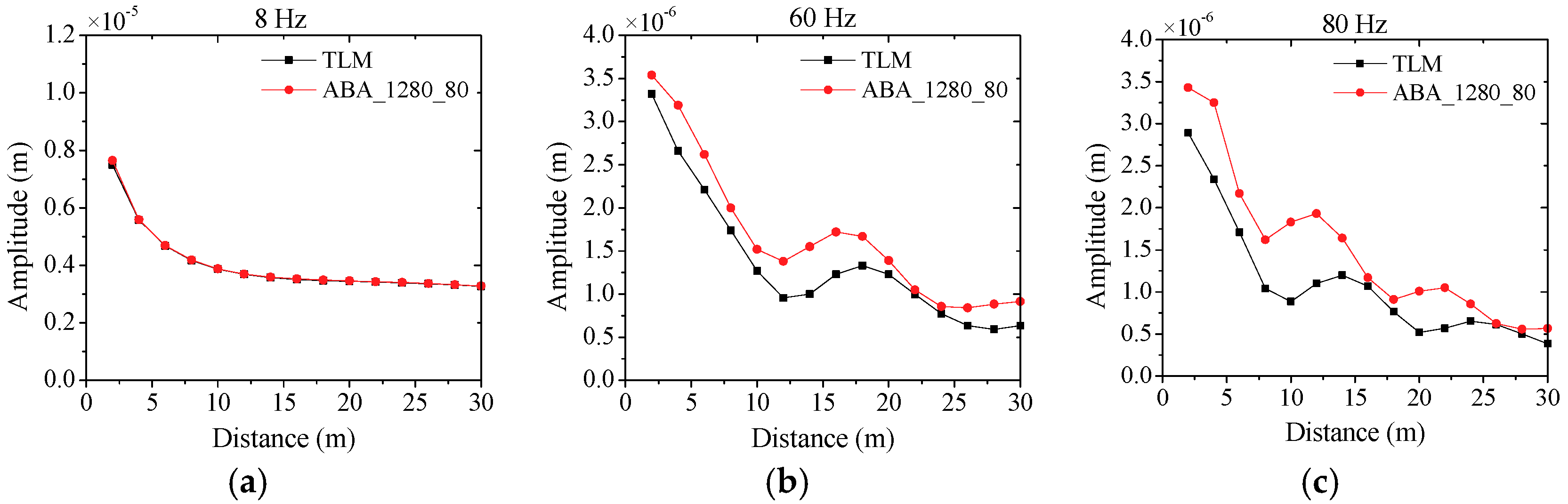
2.2. Verification of Infinite Element Method in Programs

It is an effective way to test the applicability of the presented model in different methods. The proposed finite element coupled infinite element boundary method in ABAQUS software is compared with the thin layer method (TLM), a semi-analytical and semi-numerical approach for the analysis of elastic wave propagation in stratified media [42].

An elastic half-space simulation is taken as an example in the subway induced vibration models. The basic parameters of the numerical model are as follows: the mass density ρ is 2000 kg/m³; shear wave velocity Cs is 500 m/s; Poisson’s ratio $\mu$ is 0.4; and the material damping ratio ξ of soil is 0.05. The depth of soil layer is 80 m and the base is assumed as fixed rock. The two-dimensional numerical model is built and half-structure is utilized based on symmetry in the present study. The cosine function $F=F_0\cos \left(2\pi ft\right)$, with the amplitude $F_0$ 5 kN, is applied to the models, and the applied frequency range $f$ is from 1 Hz to 80 Hz according to the required frequency band under the subway-induced vibration. The ground evaluation points are within the range of 2–30 m from the distance of load application with total 15 points and 2 m interval and the vertical vibrating displacement of these points are obtained and discussed in this section.

The base of the numerical model is fixed and the horizontal degrees are constrained on the right side. The model can be expressed as L_H, where L denotes the width of the model and H is the height (depth). The model 1280_80 notes the model width is 1280 m and the depth is 80 m. ABAQUS is abbreviated to ABA in the numerical figures.

Figure 1 presents the comparison attenuation curves at the typical frequencies of TLM and ABAQUS results with element dimension 1 m, which can be drawn that the numerical results of the two methods are similar under the low frequency load, such as 8 Hz. There are differences under the high frequency load due to the larger element dimensions. However, the differences become smaller with the finer element dimensions [35,41] in ABAQUS software, as shown in Figure 2, indicating that the finite element method is verified applicable in ABAQUS software.

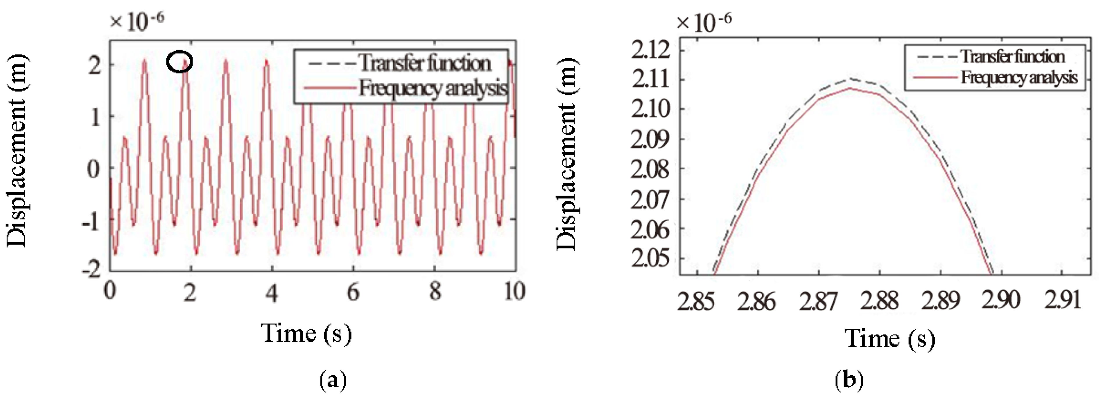
2.3. The Realization of Infinite Element Method in the Frequency Domain

To make the simulation results statistically significant, many excitations are applied to the two-dimensional, or more complex, models in the subway induced vibration, since the subway incentive is a random process. The required calculation process becomes time-consuming in the time domain analysis. Moreover, the frequency characteristics of the vibration is important in the subway induced vibration. Therefore, the numerical analysis conducted in the frequency domain is of great significance. The frequency analysis is a process of data operation, rather than the step-by-step solution process in the time history analysis. The calculation time is then saved effectively.

In this study, an interface program is developed in the commercial software ABAQUS environment. It can automatically read the simulation result files (dat file) in the ABAQUS harmonic analysis, and then the frequency domain calculation is realized by MATLAB. The main steps of frequency domain analysis could be summarized by the following:

Step 1.

The coupled finite element–infinite element boundary simulation model is built based on the commercial software ABAQUS.

Step 2.

The harmonic analyses are conducted based on the commercial software ABAQUS to obtain the amplitude and phase data of the evaluation measures on the ground in the subway induced vibration.

Step 3.

The numerical results are saved as dat file type in ABAQUS, and then read automatically by the developed interface programs to MATLAB.

Step 4.

Frequency domain analysis is performed based on MATLAB platform and the responses, such as acceleration and displacement time-histories of the evaluation points are obtained.

The simulation results acquired in Steps 1 and 2 are verified by TLM in Section 2.2. The time history with certain frequency is obtained based on the amplitude and phase, which are calculated in Step 2. Then, the total responses of evaluation points with each frequency are obtained based on the superposition principle. The frequency domain analysis in Step 4 is verified by the transfer function method, whose principle is expressed as follows:

If the transfer function $H(\omega )$ is known, then the responses of the system can be calculated by Equations (4) and (5).

$$Y(t)={\displaystyle {\int }_{-\infty }^{\infty }H(\omega )}X(\omega )e^{i\omega \mathrm{t}}d\omega$$

(4)

$$Y(\omega )=H(\omega )X(\omega )$$

(5)

where $X(\omega )$ is the frequency response functions and $Y(\omega )$ is the output Fourier transform.

Therefore, the responses of system can be calculated under any excitation $X(t)$, provided the transfer function $H(\omega )$ is known.

The correctness and the application of the program is verified by a numerical simulation, a track bed-tunnel lining-surrounding formation model, as shown in Figure 3a. Displacement load, as expressed in Equation (6), is applied to the center of the tunnel track-bed (A point) in the vertical direction. The applied displacement curve is shown in Figure 3b, and the displacement time-history of the ground surface B point is required to be calculated.

Table 1. Soil parameters of different soil layers.

Soil Layer	Thickness (m)	Depth (m)	Density (kg/m3)	Shear Wave Velocity (m/s)	Poisson’s Ratio
1	1.00	1.00	1890	74	0.35
2	3.30	4.30	1850	89	0.30
3	2.10	6.40	1850	85	0.30
4	11.26	17.66	1790	108	0.30
5	26.40	44.06	1820	220	0.25
6	2.00	46.06	1930	189	0.25
7	2.00	48.06	1940	191	0.25
8	3.40	51.46	2040	195	0.25
9	8.05	59.51	1920	230	0.25
10	16.96	76.47	1950	220	0.25
11	2.20	78.67	1920	263	0.25
12	3.78	82.45	1960	267	0.25
13	2.99	85.44	1920	272	0.25
14	6.65	92.09	1940	279	0.25
15	4.36	96.45	1930	287	0.25
16	3.55	100.00	1920	296	0.25

lists the soil parameters of different soil layers in this model.

$$x(t)=1\times {10}^{-5}[\cos (2\pi t)-2\sin (2\pi t)-2\sin (4\pi t)]$$

(6)

Figure 4 shows the comparison displacement time history of Point B by the developed interface program in frequency domain analysis and the transfer function method. The two curves almost coincide with each other, indicating that the frequency analysis is applicable in the interface programs. There is little difference between the two results in the amplified graph, as shown in Figure 4b. The reason is that the sampling points are limited in the frequency analysis, resulting in frequency leakage and numerical calculation errors.

3. Experimental Verification of the Coupled Model for Subway Induced Vibrations

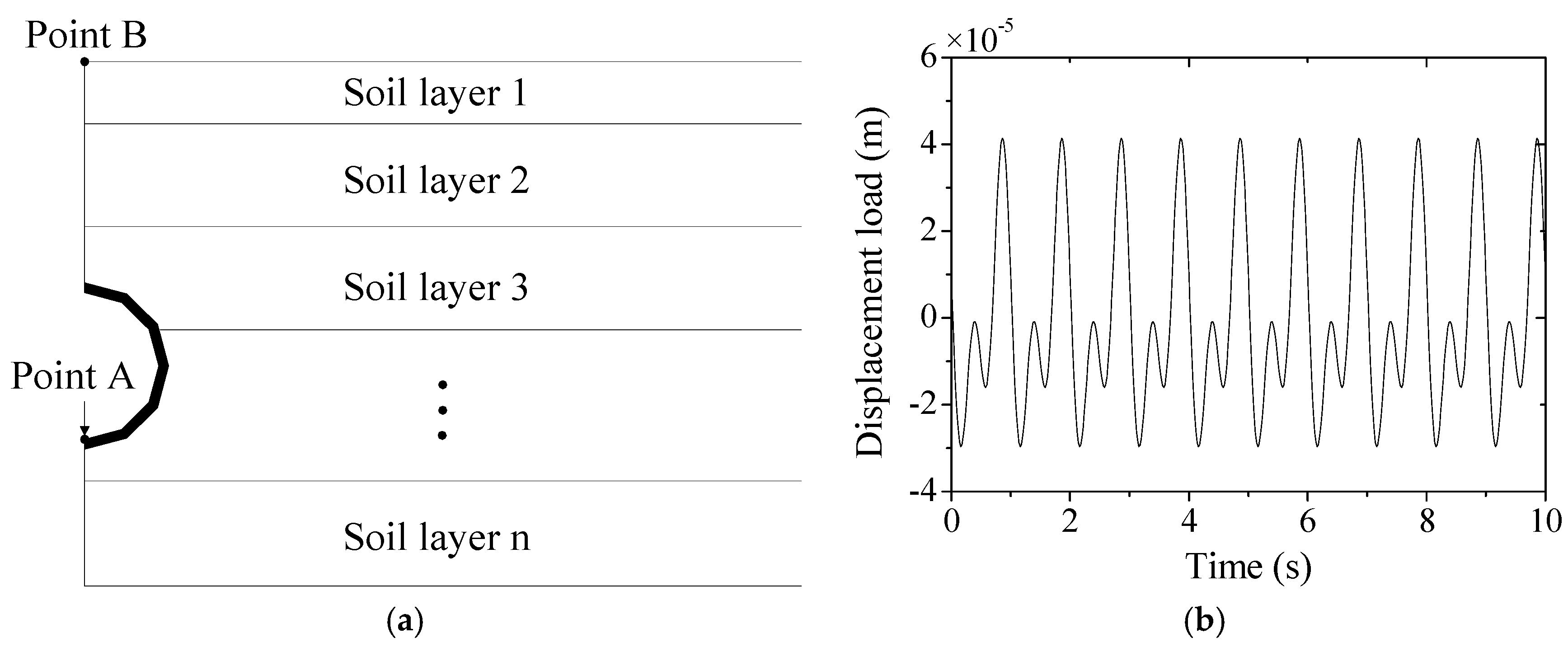
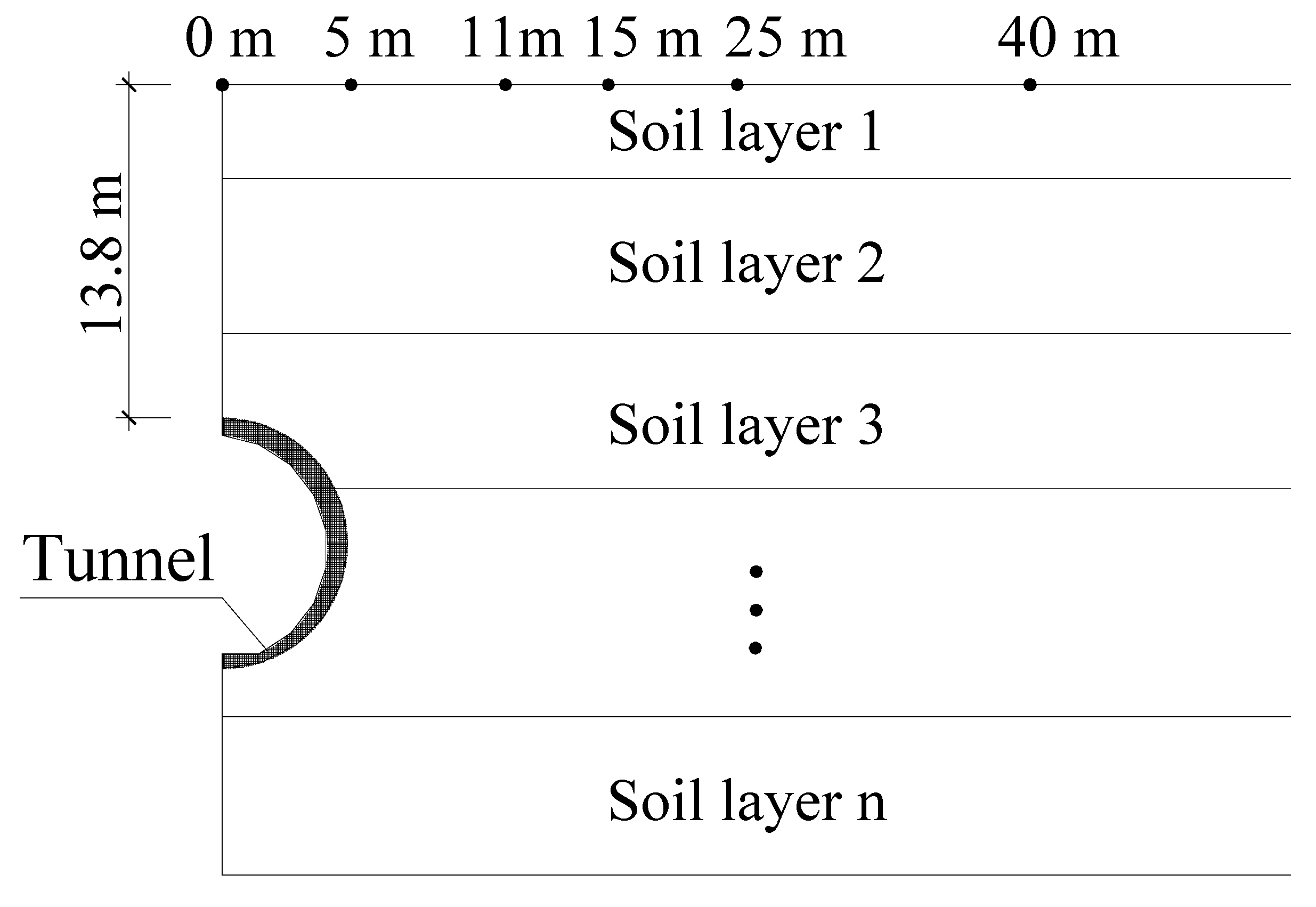
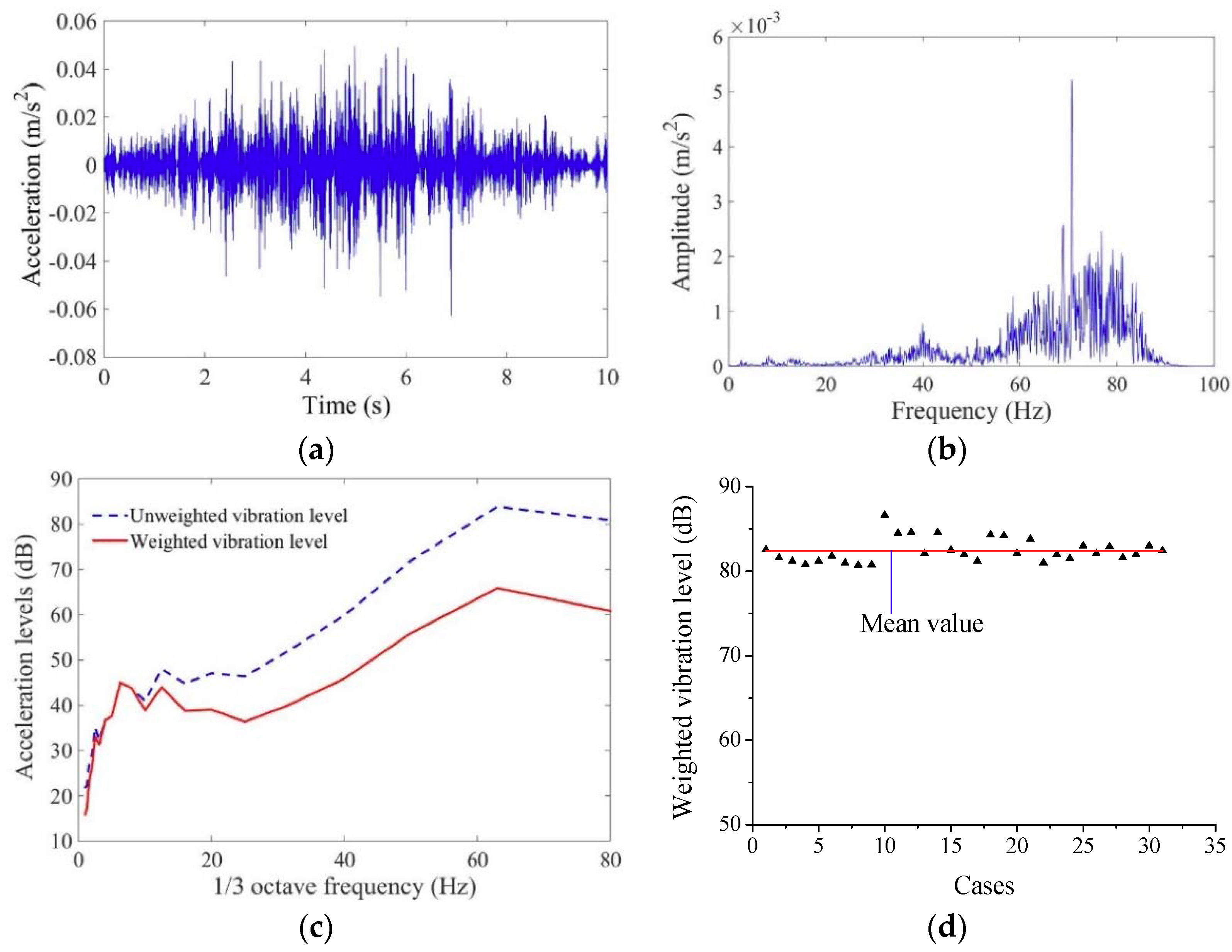
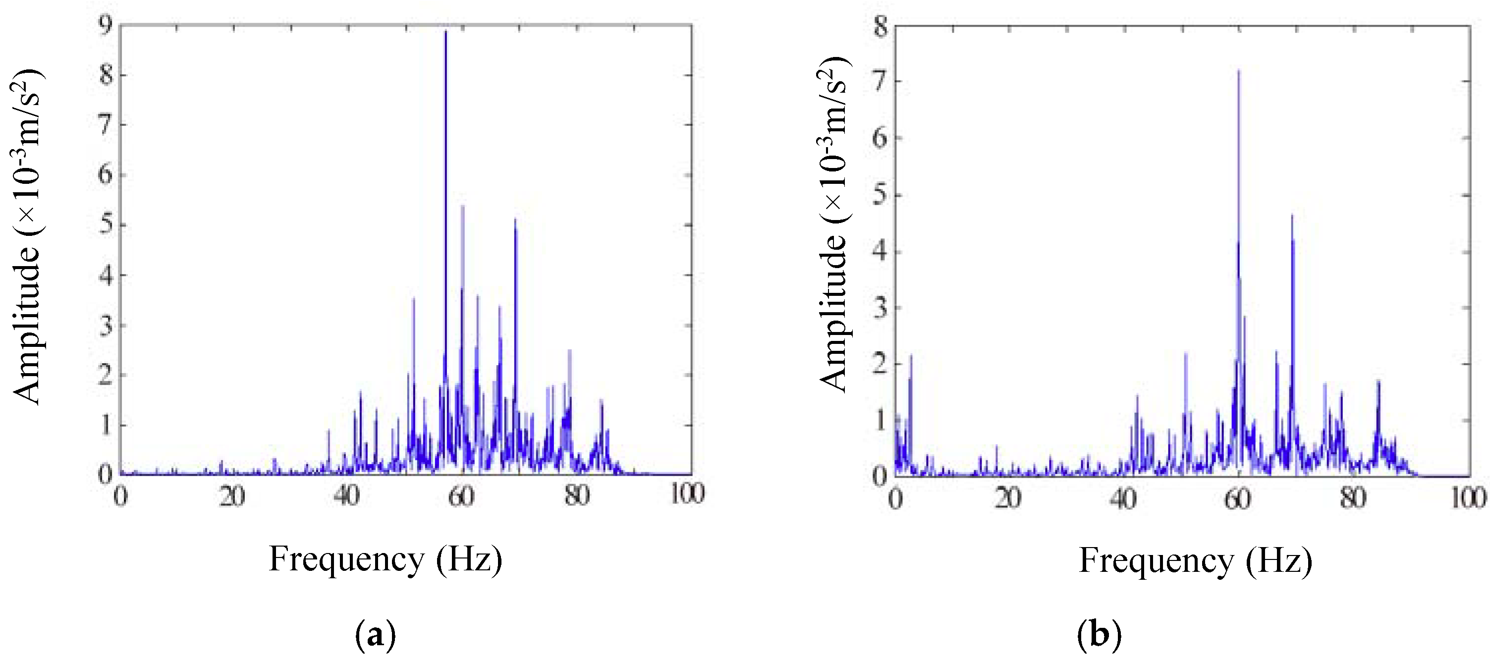
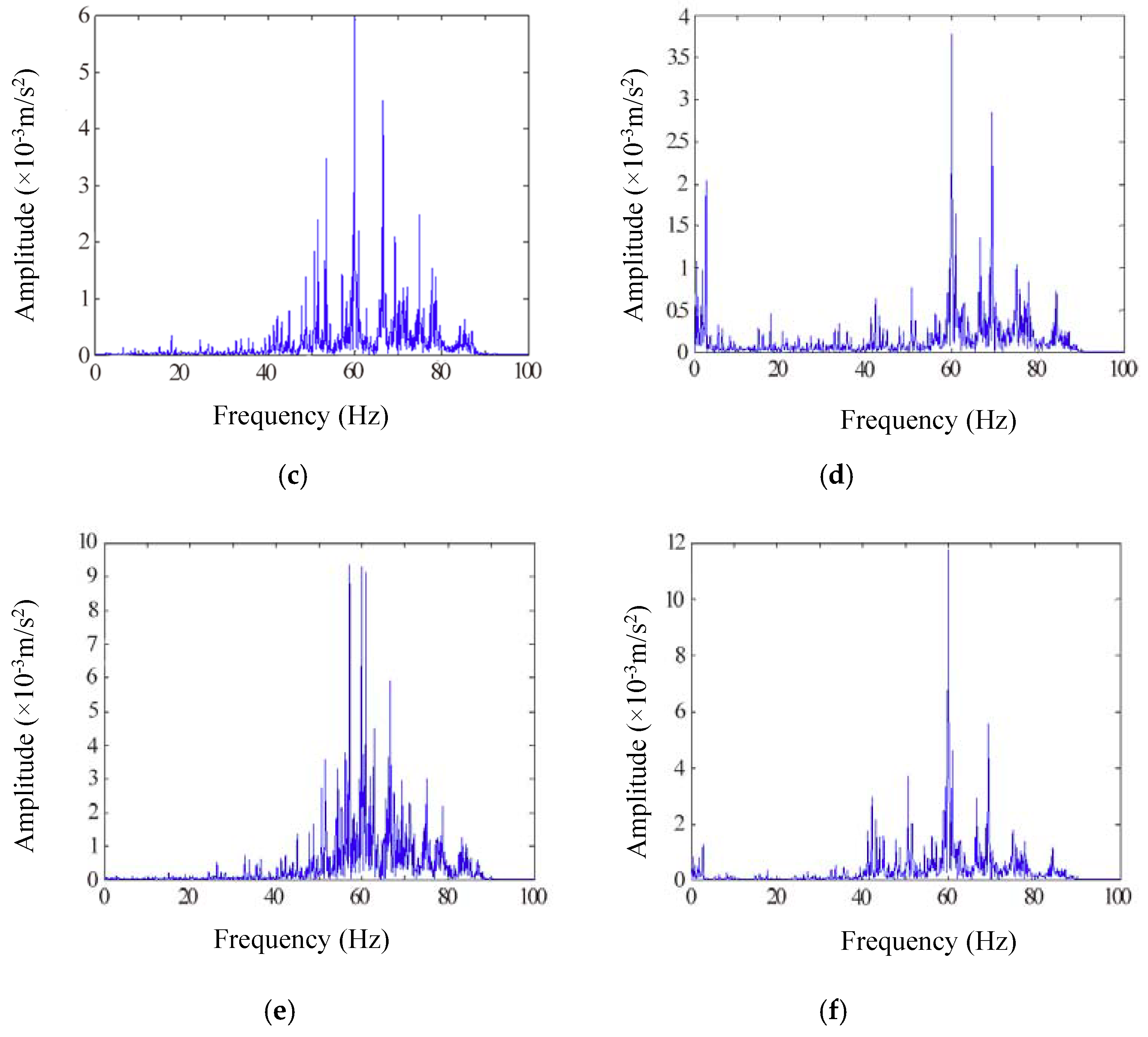
3.1. Vibration Measurement

Field measurements were performed on a track bed-tunnel lining-surrounding formation in a certain park project of Line 2, Shanghai Metro, which is an ideal test site due to the few surroundings and buildings to study the vibration attenuation characteristics of the ground surface under the subway induced vibration. The acceleration time-histories of the central tunnel and the typical ground points were measured and acquired in this test. The track bed-tunnel lining-surrounding formation model and the arrangement of measuring points in lateral direction, which were 0 m, 5 m, 11 m, 15 m, 25 m and 40 m from the central tunnel, are shown in Figure 5.

The outer radius of the tunnel is 3.1 m and inner radius is 2.75 m. The tunnel depth, the distance from the top of the tunnel to the surface of the tunnel, is 13.8 m. The elastic modulus, the density and Poisson’s ratio of concrete are 34,500 MPa, 2500 kg/m³ and 0.25, respectively. The typical clay in Shanghai, not homogeneous in the depth direction, was employed in this field test and numerical simulation. The soil parameters of different soil layers are shown in Table 1 in Section 2.3.

The 31 accelerations of the evaluation points in the center of the track bed were measured and acquired in this field test, with total excitation time 10 s and sample frequency 200 Hz. The 31 accelerations correspond to 31 cases. The typical acceleration time history of the track bed, its corresponding Fourier spectra and 1/3 octave frequency are provided in Figure 6a–c, in which it can be observed that the dominant frequencies of the tunnel track bed induced by the subway are above 40 Hz. The measured results agree with other tests [43] that the vibration frequency induced by the subway is high. Vibration level of each recorded accelerations is shown in Figure 6d based on the Shanghai regulation, in which it can be seen that the vibration level is within 80–85 dB and the mean value is 82.4 dB.

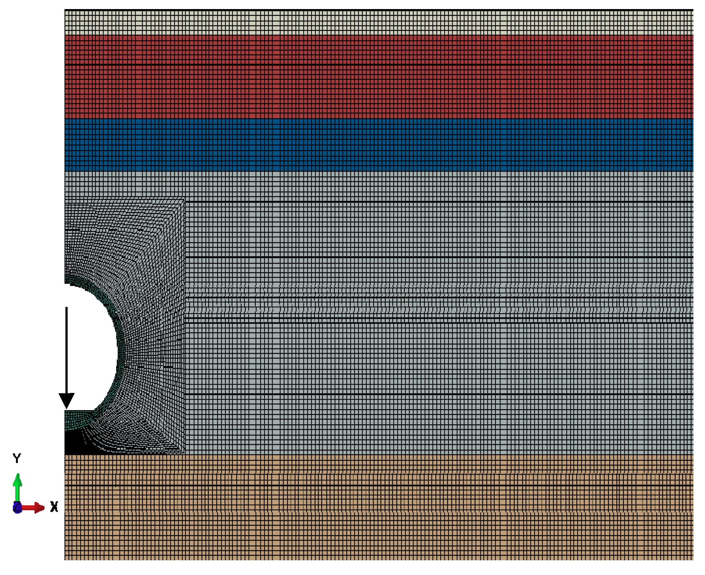
3.2. The Coupled Finite Element–Infinite Element Boundary Model

In this engineering, the minimum wave velocity of the soil is 100 m/s, the width of the finite element region is designed as 100 m, and the model depth is 100 m. Infinite element boundary is applied to the right side and the bottom of the models. The element size in this engineering along the horizontal direction and vertical direction within 50 m depth is designed as 0.2 m, while other regions are meshed with 0.4 m. The tunnel is analyzed with plane strain solid elements, with the element size 0.1 m × 0.1 m (width and height). The measured 31 accelerations of the evaluation points in the center of the track bed are applied vertically to this position in the simulation model. The simulation frequency is 0–100 Hz, with 0.1 Hz interval. The simulation points are within 0–40 m of the center of the tunnel, coincident to the measure points displayed in Figure 5. The meshed model of track bed-tunnel lining-surrounding formation is shown in Figure 7. The numerical results are obtained by the harmonic analysis in ABAQUS software and frequency analysis in MATLAB, connecting by the developed interface programs, as introduced in Section 2.3. Soil behaviors are simplified in this simulation model and soil properties are based on the practical engineering, as shown in Table 1.

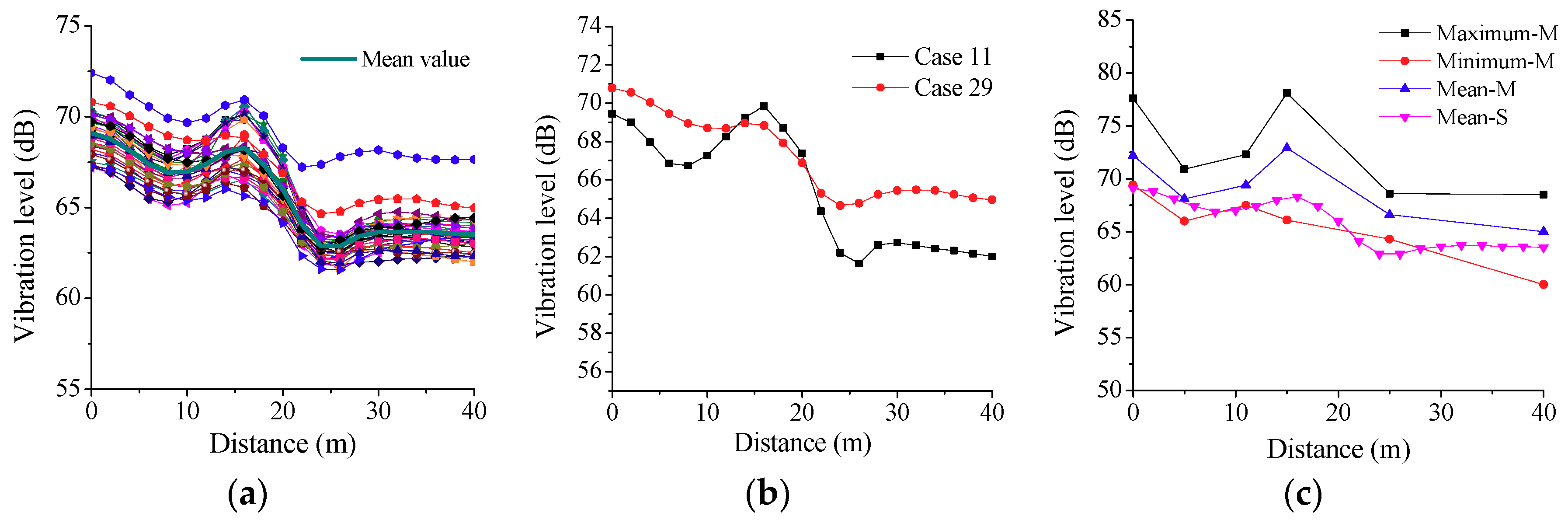
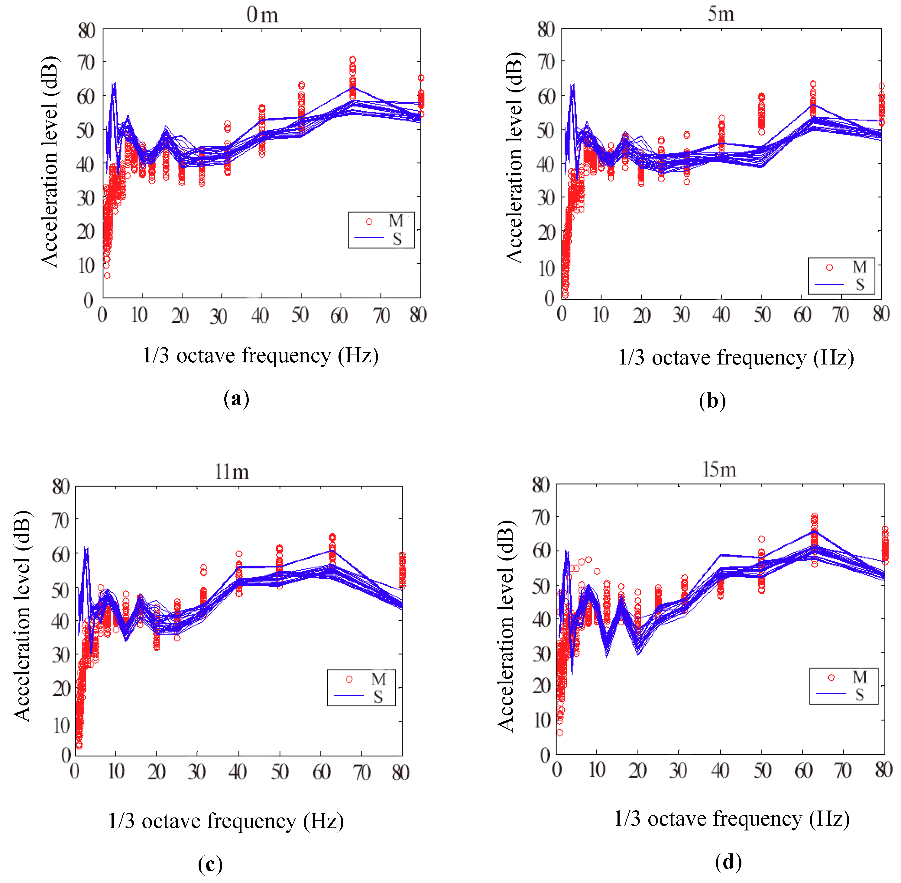
3.3. Numerical Results

The simulation attenuation of peak vibration levels in the vertical direction with respect to distance under the 31 measured accelerations excitations are shown in Figure 8a,b. In addition, the mean attenuations of peak vibration levels, which are obtained by the measurement and simulation, are compared in Figure 8c. The following conclusions can be drawn.

The attenuation curves of vibration levels generally decrease with the increasing distance away from the central tunnel. However, there exists an amplifying area of vibration that the vibration level at 10 m from the center is about 5 dB greater than that at 15 m.

This amplification effect due to the wave propagation and reflection is consistent with the results of measurement and numerical simulation obtained by other researchers [44]. If the reflection frequency is dominant and obvious in the applied frequency components, the overall vibration will reflect due to the wave superposition in this area. A part of the vibration wave is directly transmitted through the bound site, and part of the wave first spreads to the ground surface and then propagates from the ground to the lateral sides, forming a superposition effect in this area. This may result in a larger vibration in this field than that directly above the tunnel. The wave propagation phenomenon is clearly observed in the measured ground data by Takemiya [7].

Moreover, the amplification phenomenon is obvious in some cases, such as in Case 11, while some are not apparent, such as in Case 29, as shown in Figure 8b, indicating that the amplification has relationship with the spectrum of the applied excitation accelerations.

The numerical mean value of vibration level basically maintains within the measured range, which is a little smaller than the mean value of experimental results, as shown in Figure 8c. The amplification of vibration level is also obtained in the simulation, about 15 m away from the center of the tunnel.

Figure 9 plots the simulation and measurement frequency spectra 0 m, 5 m and 15 m from the center tunnel. The calculated and measured frequency spectra, with dominant frequency 40–90 Hz, are generally similar. The frequencies are consistent with the findings by Kaewunruen that most vibration issues are between 2 and 150 Hz for the neighborhood near railway lines in tunnels, on embankments, in a cutting or on the level ground [14]. In addition, there is a peak value within 5 Hz in the simulation, which is different from the measurement. The reason is that there is a fundamental frequency in the numerical model due to the limited element dimensions, and amplification effect generates as the excited frequency is close to the model’s basic frequency.

Figure 10 displays the compassion 1/3 octave band frequency spectra of simulation with the letter S drawn by the blue lines and measurement with the letter M to show the trend of the vertical response at the distance of 0 m, 5 m, 11 m and 15 m to the central tunnel (as shown in Figure 5). In Figure 10, the calculated acceleration vibration levels are larger than that in the measurement as the 1/3 octave frequency is smaller than 5 Hz, which is mainly due to the amplification effect. On the other hand, the simulation vibration levels are consistent with the measurement in the higher frequencies, in which the trend of the 1/3 octave band frequency spectra by the observation and simulation results agree with the in-situ vibration measurements [7] and the observations on the waiting platform in Boston [45]. Generally, the directivity differences in the measurement and simulation frequencies are small, demonstrating that the coupled finite element–infinite element boundary method can better capture the vibration characteristics in practical engineering, since the frequency of subway-induced vibration is high [43].

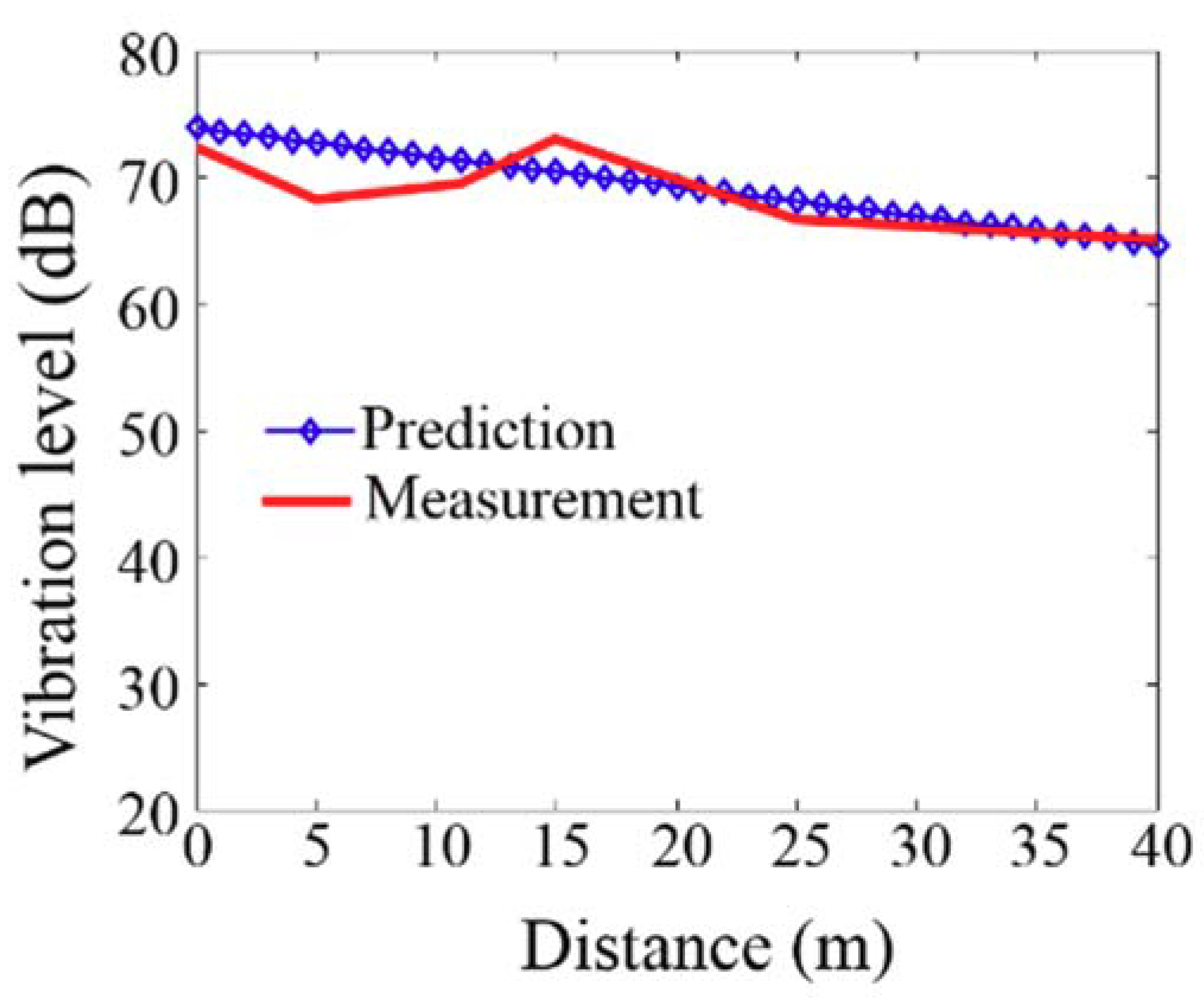
3.4. Simplified Prediction Formula of Ground Vibration Level

The ground vibration level is mainly influenced by the tunnel track-bed vibration and the tunnel depth. A simplified prediction formula of the ground vibration level of the track bed-tunnel lining-surrounding formation on this engineering certain soft site, based on the numerical simulation models with different tunnel depths and the track-bed accelerations, is presented as Equation (7).

$$V{L}_Z=V{L}_{ZS}(-0.0028x-0.0033h+0.942)$$

(7)

where $V{L}_Z$ is the ground vertical acceleration level (dB), and $V{L}_{ZS}$ is the tunnel track-bed vertical acceleration level (dB). $x$ is the horizontal distance away from the center of the tunnel (m), and $h$ is the tunnel depth (m).

Figure 11 plots the attenuation of peak vibration levels with respect to distance in this practical engineering. The predicted vibration levels are approximately similar to the measured results, with maximum error 3 dB. Therefore, the proposed prediction formula is acceptable and applicable for the prediction of vibration levels induced by subway in the practical engineering.

4. Parametric Study of Coupled Finite Element-Infinite Element Boundary Method in the Subway Induced Vibration

The elastic half-space simulation introduced in Section 2.2 is used in this section to discuss the efficiency of the presented finite element method coupled infinite element boundary and the parametric study is conducted to investigate the influence of model widths and depths on the numerical results.

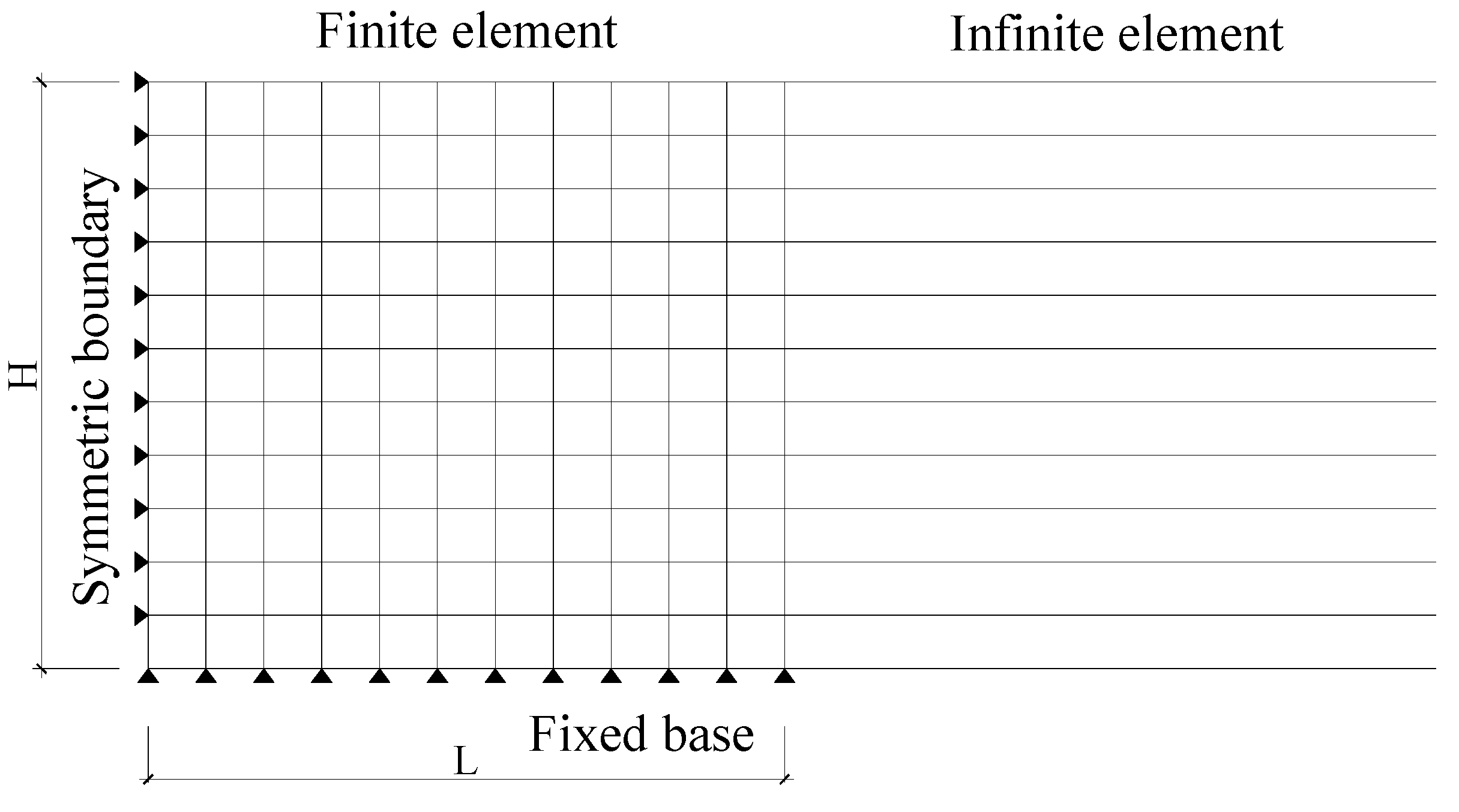
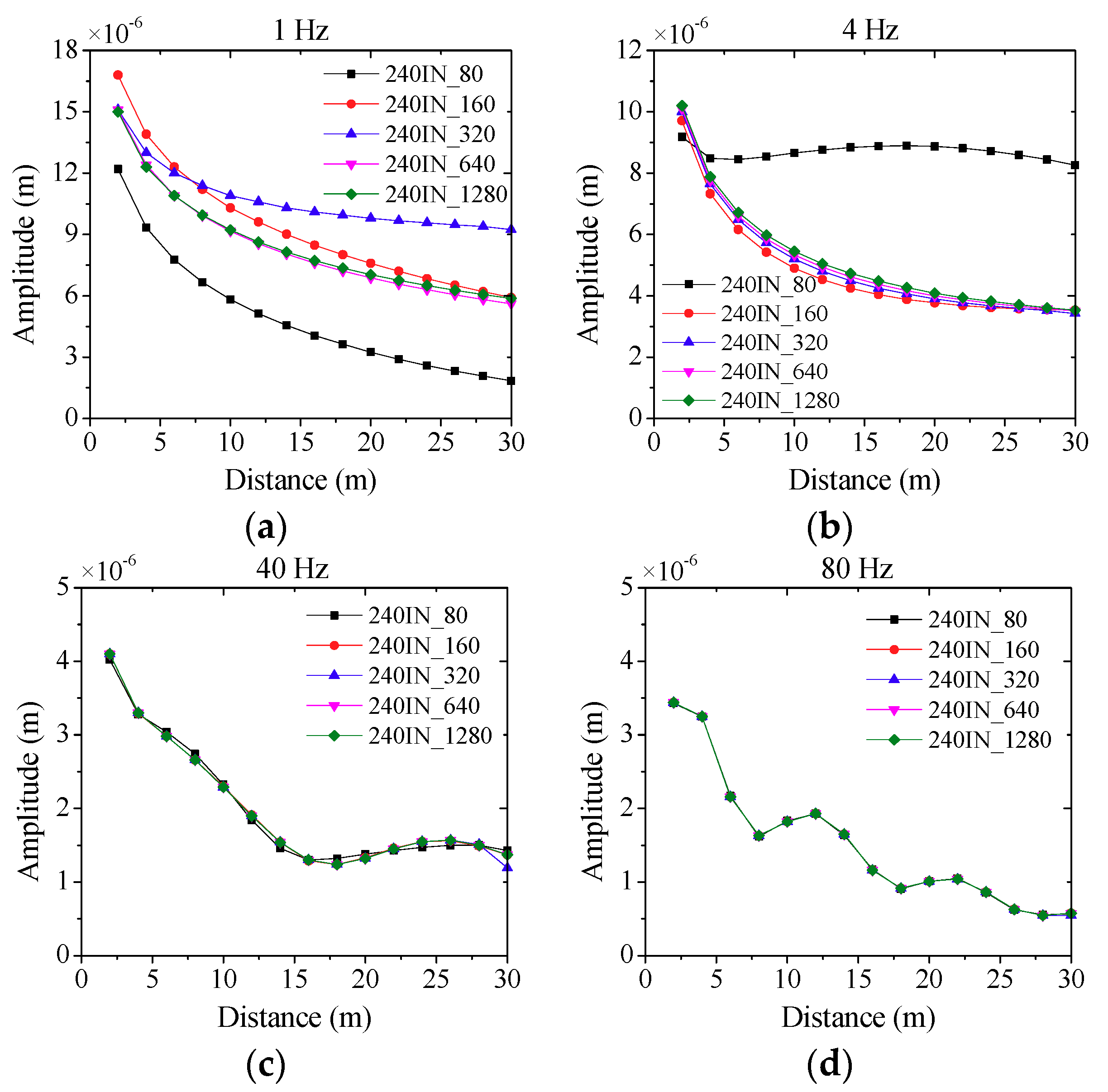
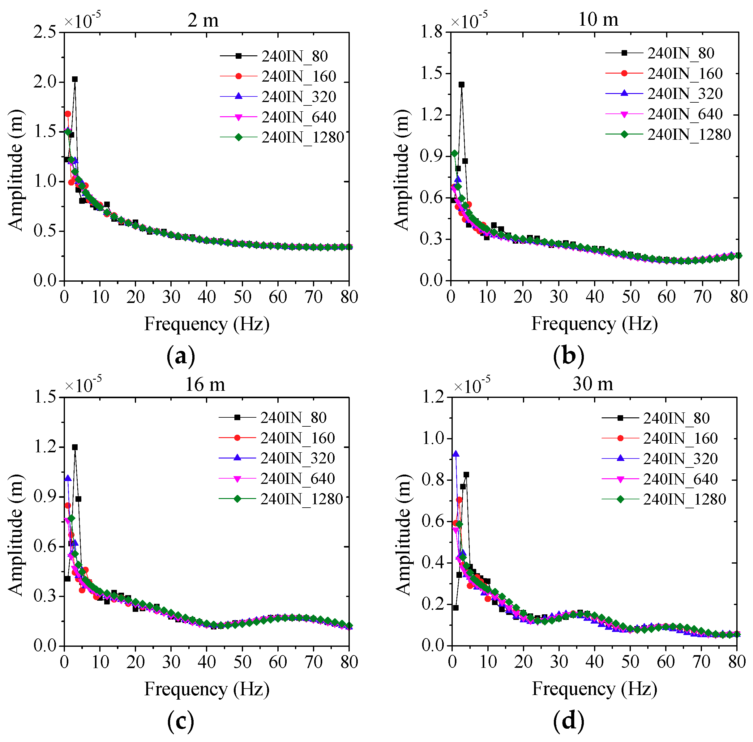
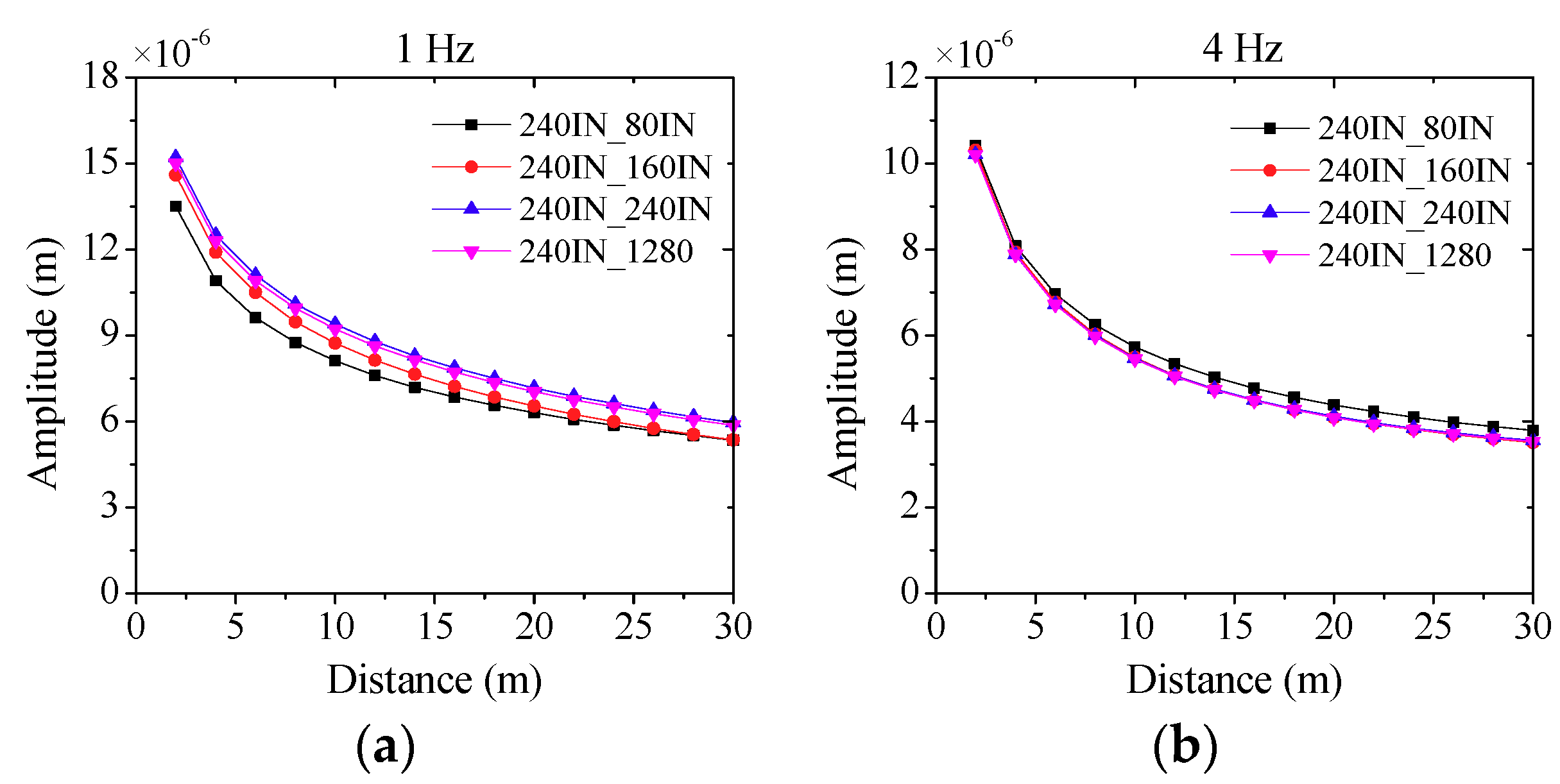
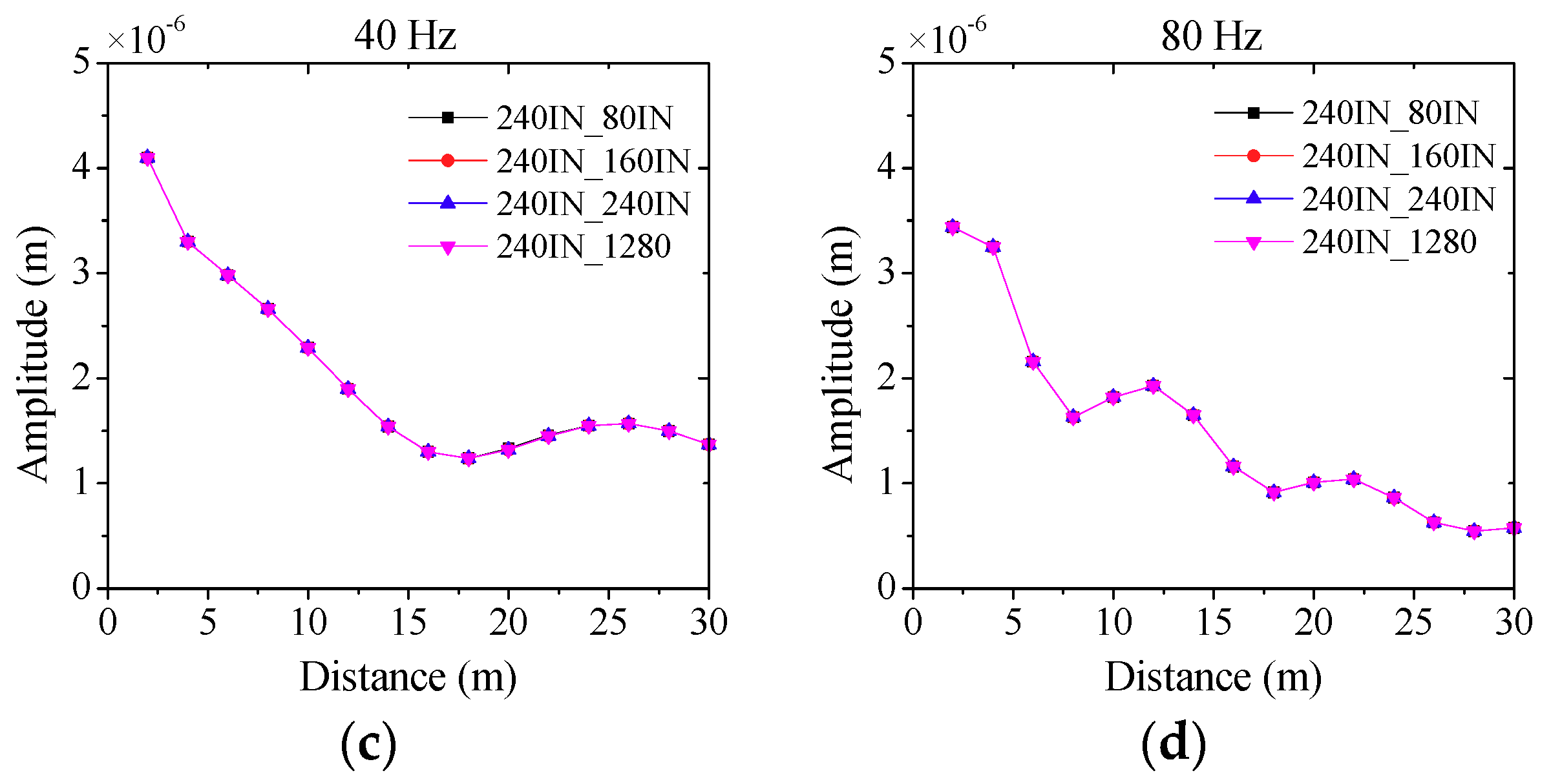
4.1. The Effect of Model Depths on the Simulation Results

Table 2. Numerical cases with different model depths.

Case	1	2	3	4	5
L × H (m × m)	240 × 80	240 × 160	240 × 320	240 × 640	240 × 1280
Expression	240IN_80	240IN_160	240IN_320	240IN_640	240IN_1280

shows the numerical cases with different model heights. The model can be expressed as LIN_H, where L denotes the width of the model, H is the height and IN means that the infinite element is adopted to the lateral side of the model. The base of the model is fixed in the simulation. The dimension of the element is 1 m × 1 m. Plain strain element CPE4 is used as the finite element in this model. Different model depths are analyzed to obtain a stable solution. Figure 12 is the sketch of the model with infinite element. Symmetrical constraints are imposed on the left boundary and the infinite element is applied to the right side of the model.

The attenuation curves of the model applied to lateral infinite element boundary with different heights under the excitations of different vibration frequencies are shown in Figure 13. The numerical results of models with different heights are similar under the high frequency load, such as 40 Hz and 80 Hz, while the results are obviously different under the low frequency load. The numerical errors compared to the benchmark model 240IN_1280 mainly depend on the vertical frequencies, using an equation $f_0=c_p/4H$, with 3.8 Hz, 1.9 Hz, 0.95 Hz, 0.48 Hz and 0.24 Hz of the models in Cases 1–5, respectively. Therefore, the vertical frequencies of the models are small, resulting relative larger errors under low frequency load (close to the vertical fundamental frequency) than that under high frequency load. Vertical frequency, depending on the depth of the model with certain soil property, has great influence on the simulation results. Therefore, the depth of the model should be designed seriously to reduce the numerical errors due to the improper depth of the model. This agrees with the conclusion obtained by Andersen [46] that the accuracy of the simulation results increases with the distance from the tunnel; in other words, the depth of the model is significant to obtain more accurate estimates.

Figure 14 shows the amplitude–frequency curve of the models with different heights. It can be observed that: (1) There is an obvious peak in the curve when the model height is 80 m, while the amplitude–frequency curves are monotonic in other models. This is because the vertical frequency becomes smaller with the increase of model depth, and the vertical frequencies are less than 1 Hz to most models. However, the applied frequencies are equal to or greater than 1 Hz, larger than the vertical frequency. Therefore, there are no obvious peak values of most models in the amplitude–frequency curve. (2) The frequencies corresponding to the maximum error of the amplitude–frequency curves are mainly in the low frequency (1–6 Hz). Moreover, the error of amplitude–frequency curve is less than 5% when the model height is 640 m, indicating that numerical results are stable.

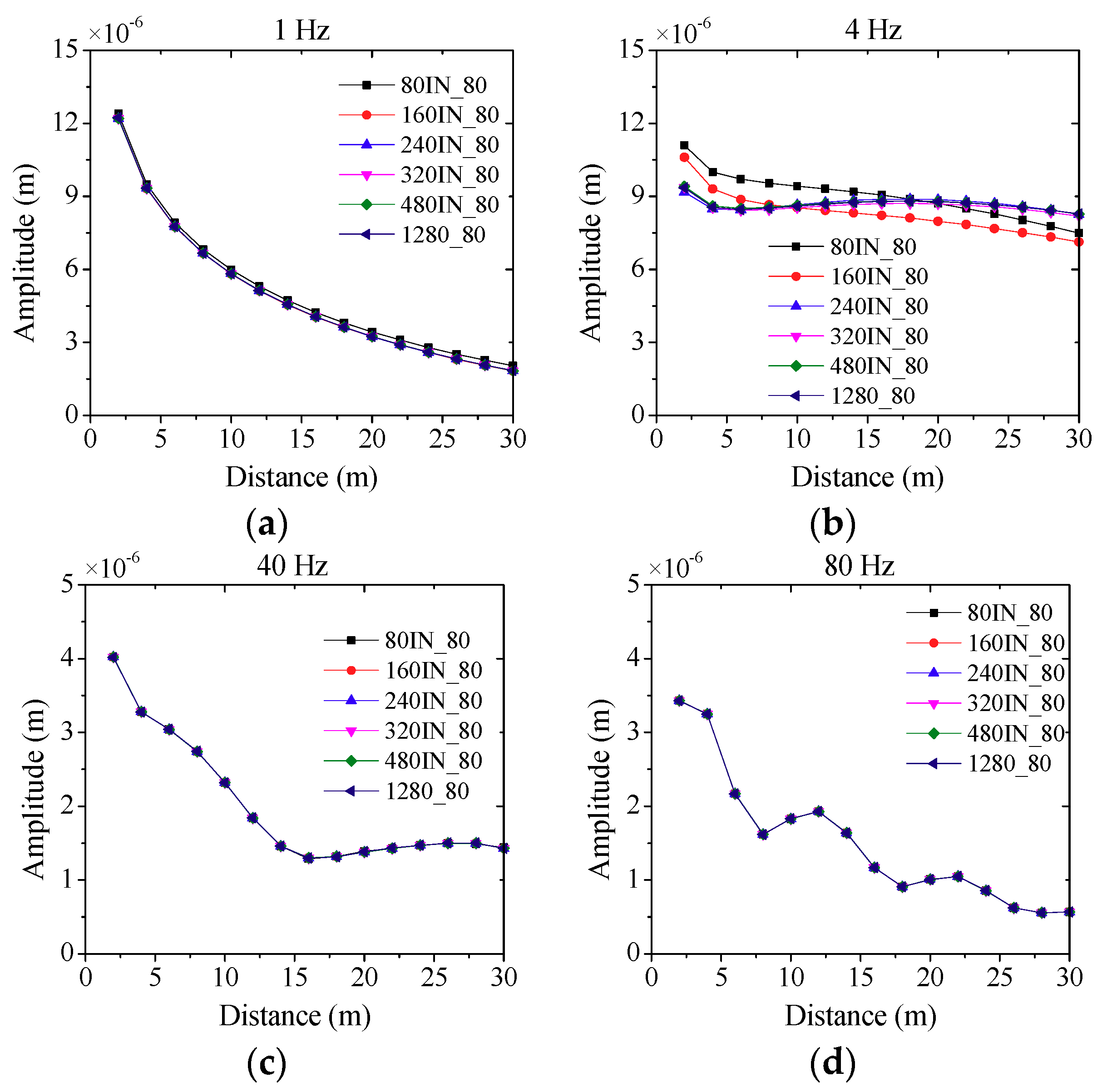
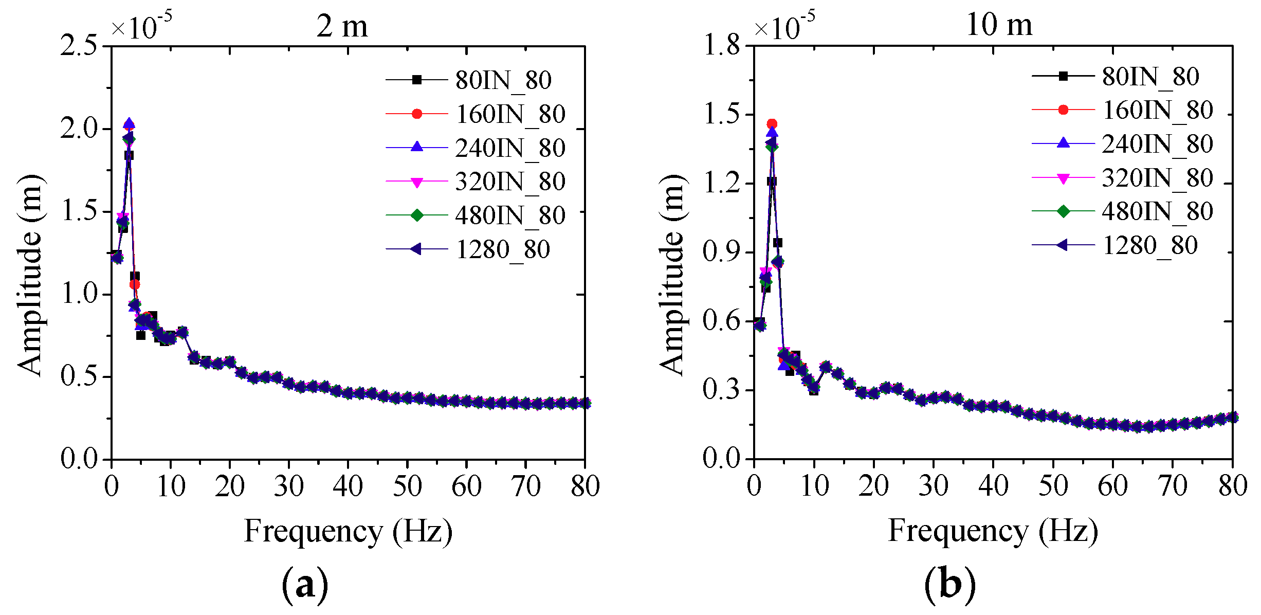
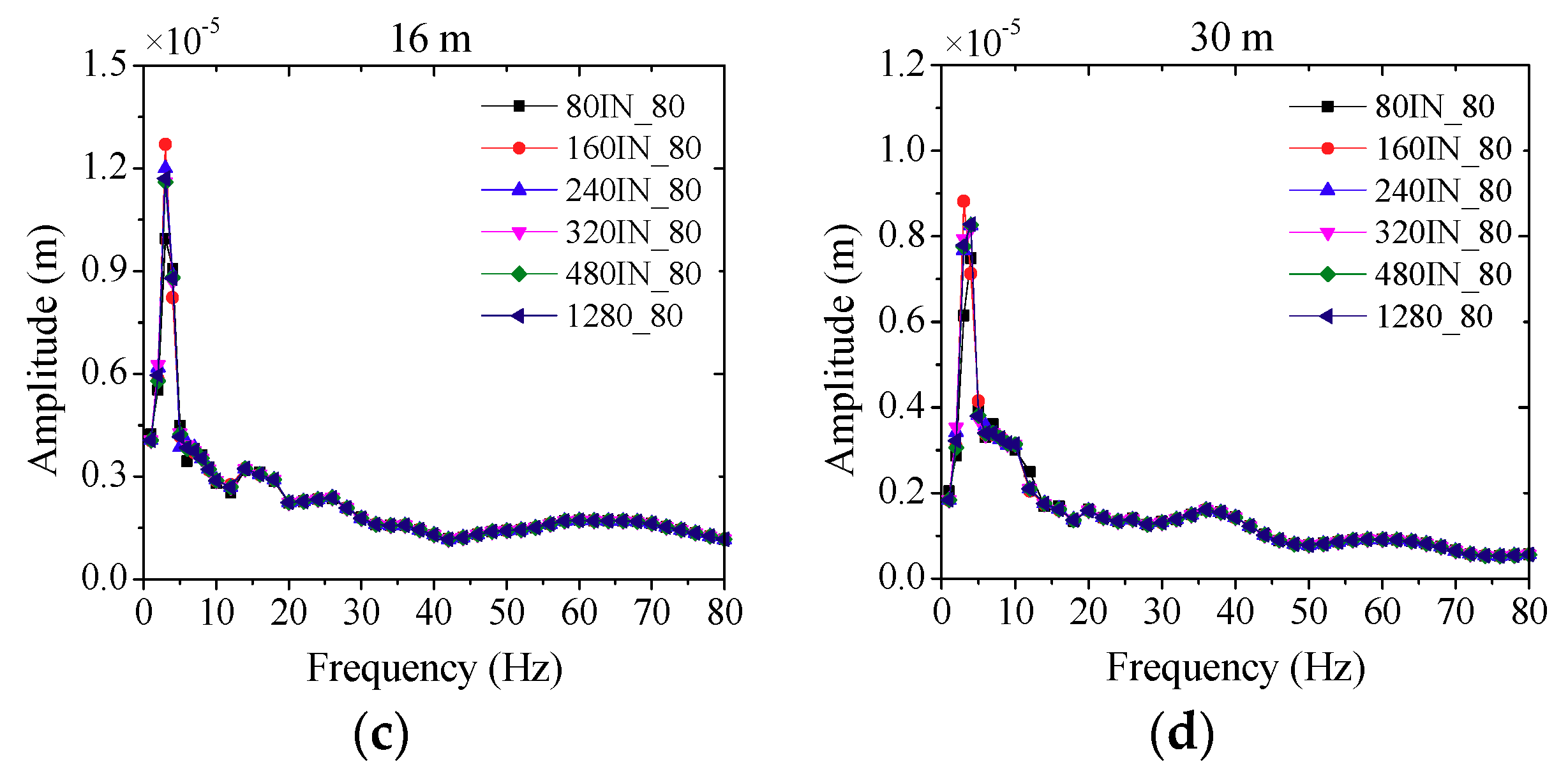
4.2. The Effect of Model Lateral Sides with Infinite Element Boundary on the Simulation Results

Table 3. Numerical cases of different model widths with lateral infinite element.

Case	1	2	3	4	5
L × H (m × m)	80 × 80	160 × 80	240 × 80	320 × 80	480 × 80
Expression	80IN_80	160IN_80	240IN_80	320IN_80	480IN_80

shows the numerical cases of models with lateral infinite element. The applied boundary is similar to the models in Section 4.1. In this section, the model height remains unchanged to study the influence of model width on the numerical results with the infinite element applied to the lateral side.

The numerical simulation shows that the solution is stable with the model width 1280 m, based on the discussion in Section 2.2. Therefore, the result of model 1280_80 is used as a benchmark to be compared with other models’ results in this section.

The attenuation curves of the infinite element model with different widths under the excitation of vibration frequencies are shown in Figure 15. It can be seen that: (1) There is a certain requirement on the dimensions of the finite element area with the infinite element boundary applying to the lateral side, since smaller finite element area generates greater calculation error. While with the increasing of width in the finite element area, the calculation results tend to be stable gradually. (2) The simulation errors of finite element model 160_80 and model 160IN_80 are 60.78% and 13.88%, respectively, indicating that the maximum error is significantly reduced with the infinite boundary. The finite element model notes that infinite element boundary is not applied to the model. The relative error is the simulation results comparison with that in the benchmark model 1280_80.

Figure 16 shows the amplitude–frequency curve of the models with different widths and the infinite element boundary is applied to the lateral side in the simulation models. It can be observed that the errors of the infinite element model with 480 m width is less than 5%, and when the model width is 320 m, its corresponding error is 10%. The widths of the finite element model are 960 m and 640 m, respectively, to obtain the same accuracy. Therefore, the horizontal dimension of the finite element area can be reduced 50% effectively by means of the infinite element boundary, and the calculation accuracy remains unchanged. Moreover, the computational time can be saved due to the decreasing number of element units, demonstrating the higher performance of the combined finite element–infinite element boundary method.

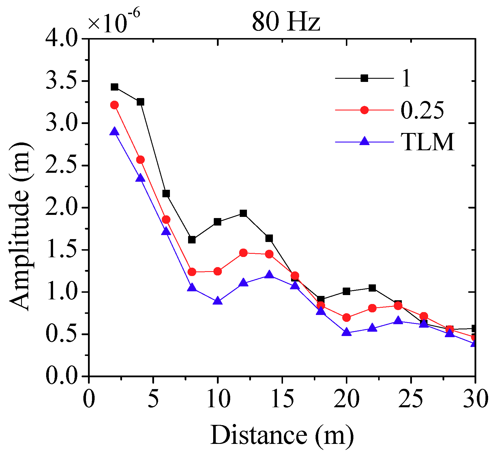
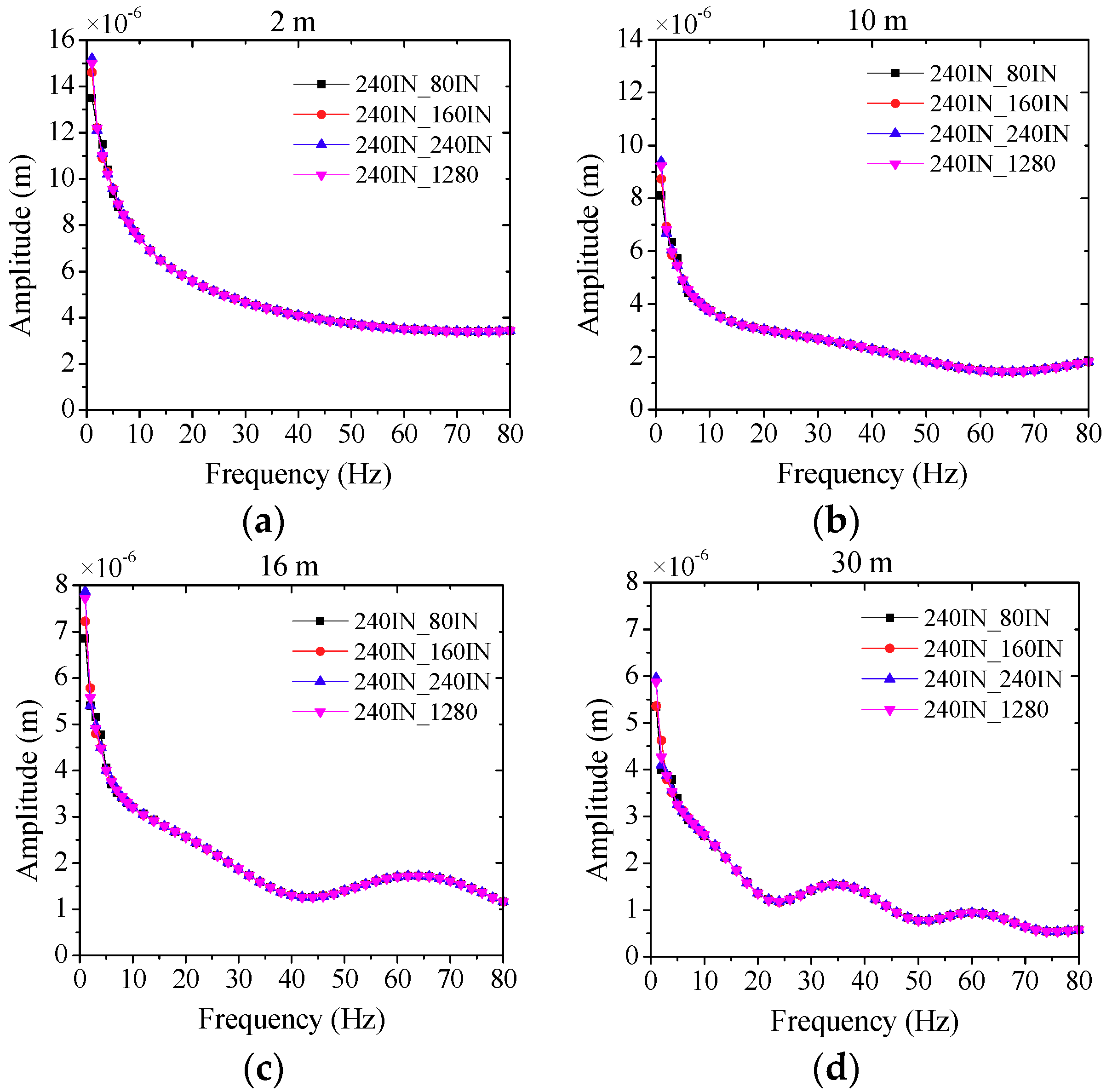
4.3. The Effect of Model Base with Infinite Element Boundary on the Simulation Results

Table 4. Numerical cases of different model depths with base infinite element.

Case	1	2	3
L × H (m × m)	240 × 80	240 × 160	240 × 240
Expression	240IN_80IN	240IN _160IN	240IN_240IN

shows the numerical cases with different model depths. The model can be expressed as L IN_H IN. The infinite element is applied to the right side and the base of the model. In these cases, the model width remains unchanged to study the influence of model depth on the numerical results with the infinite element. The numerical simulation shows that the solution is stable when the model’s height is 1280 m based on the discussion in Section 4.1. Therefore, the result of model 240IN_1280 is used as a benchmark to be compared with other model results in this section.

The attenuation curves of the infinite element models with different heights under the excitation of vibration frequencies are shown in Figure 17, from which it can be concluded that there is a relatively large difference between the calculated curve and the stable solution under the low frequency excitation when the model depth is small. However, the results are close to the stable solution under the high frequency excitation, such as 40 Hz. Therefore, larger height and higher frequency load generally generate smaller simulation errors.

Figure 18 shows the amplitude–frequency curve of the models with different heights as infinite element boundary is applied to the lateral side and base of the model. It can be observed that the results of amplitude–frequency in the infinite element models are much closer to the stable solution compared with that in Figure 14 in Section 4.1. The reason is that the fundamental frequency of the infinite models decreases, close to that of benchmark 240IN_1280. In addition, from the energy point of view, the reflection energy becomes weaker and close to the half-space infinite body after applying the infinite-element boundary. The near-source induced waves usually contain high energy, which may cause greater vibration [44].

Moreover, the model 240IN_640 in Section 4.1 can be replaced by the model 240IN_240IN in this section to achieve the same calculation accuracy, demonstrating that the height of finite element model can be reduced 62.5% after applying the infinite element boundary to the model base. Meanwhile, computational time is saved effectively, revealing the high performance of the coupled finite element–infinite element boundary method in decreasing the models’ dimensions once more.

5. Conclusions

In this study, a coupled finite element–infinite element boundary model based on the basic principles of the infinite element method was performed by the harmonic analysis based on the commercial software ABAQUS to address the issue of subway induced vibration, a major environmental concern in urban areas. In addition, the finite element method in the harmonic analysis was verified by comparing it with the thin layer method. Moreover, an interface program was developed to automatically read the simulation result files (dat file) in the ABAQUS harmonic analysis, and then the data were put into the frequency domain calculation on the MATLAB platform. Besides, a measurement of a practical engineering was performed on a track bed-tunnel lining-surrounding formation located on Line 2, Shanghai Metro, and the corresponding simulation model was established based on the introduced method. In this paper, the numerical results of vibration level and spectrum characteristic are discussed. Moreover, a simplified prediction formula of ground vibration level is proposed based on the measurement results. Finally, parametric study was conducted in an elastic half-space simulation to investigate the influence of model widths and depths with infinite element boundary on the numerical results, demonstrating the effectiveness and high performance of the coupled finite element–infinite element boundary model in the harmonic analysis based on ABAQUS. The following are the conclusions drawn from this study, which may provide insight towards the rational models of subway induced vibration.

• The coupled simulation method is applicable for the practical engineering projects of subway induced vibration on the soft site in Shanghai, and the proposed formula for the vibration levels is reasonable for the prediction in the subway induced vibration.
• There exists a vibration amplifying zone a certain distance from the tunnel under high frequency loads due to wave propagation and reflection, and the amplification has relationship with the spectrum of the applied excitation accelerations.
• The finite element model dimensions can be reduced 50% and 66.67% effectively in the widths and depth, respectively, with the coupled method, applying the infinite element boundary to the lateral and base sides of the finite element model.
• The model dimensions have great influence on the numerical results as the excited frequency is close to the model’s vertical fundamental frequency, and the depth of the model should be designed seriously to reduce the numerical errors.

References

1. Xia, H.; Cao, Y.M. Problem of railway traffic induced vibrations of environments. J. Railw. Sci. Eng. 2004, 1, 44–51. (In Chinese) [Google Scholar]
2. Gupta, S.; Degrande, G.; Lombaert, G. Experimental validation of a numerical model for subway induced vibrations. J. Sound Vib. 2009, 321, 786–812. [Google Scholar] [CrossRef]
3. Gupta, S.; Liu, W.F.; Degrande, G.; Lombaert, G.; Liu, W.N. Prediction of vibrations induced by underground railway traffic in Beijing. J. Sound Vib. 2008, 310, 608–630. [Google Scholar] [CrossRef]
4. Lopez-Mendoza, D.; Romero, A.; Connolly, D.P.; Galvin, P. Scoping assessment of building vibration induced by railway traffic. Soil Dyn. Earthq. Eng. 2017, 93, 147–161. [Google Scholar] [CrossRef]
5. Zhong, H.; Qu, D.; Lin, G.; Li, H.J. Application of sensor networks to the measurement of subway-induced ground-borne vibration near the station. Int. J. Distrib. Sens. 2014. [Google Scholar] [CrossRef]
6. Sun, K.; Zhang, W.; Ding, H.; Kim, R.E.; Spencer, B.F. Autonomous evaluation of ambient vibration of underground spaces induced by adjacent subway trains using high-sensitivity wireless smart sensors. Smart Struct. Syst. 2017, 19, 1–10. [Google Scholar] [CrossRef]
7. Takemiya, H. Analysis of wave field from high-speed train on viaduct at shallow/deep soft grounds. J. Sound Vib. 2008, 310, 631–649. [Google Scholar] [CrossRef]
8. Liu, C.; Wei, J.H.; Zhang, Z.X.; Liang, J.S.; Ren, T.Q.; Xu, H.Q. Design and evaluation of a remote measurement system for the online monitoring of rail vibration signals. Proc. Mech. Eng. Part F 2016, 230, 724–733. [Google Scholar]
9. Li, X.H.; Long, Y.; Ji, C.; Zhong, M.S.; Zhao, H.B. Study on the vibration effect on operation subway induced by blasting of an adjacent cross tunnel and the reducing vibration techniques. J. Vibroeng. 2013, 15, 1454–1462. [Google Scholar]
10. Ling, X.Z.; Chen, S.J.; Zhu, Z.Y.; Zhang, F.; Wang, L.N.; Zou, Z.Y. Field monitoring on the train-induced vibration responses of track structure in the Beiluhe permafrost region along Qinghai-Tibet railway in China. Cold Reg. Sci. Technol. 2010, 60, 75–83. [Google Scholar] [CrossRef]
11. Kouroussis, G.; Florentin, J.; Verlinden, O. Ground vibration induced by intercity/inter region trains: A numerical prediction based on the multibody/finite element modeling approach. J. Vib. Control 2016, 22, 4192–4210. [Google Scholar] [CrossRef]
12. Kaewunruen, S.; Remennikov, A.M. Sensitivity analysis of free vibration characteristics of an in situ railway concrete sleeper to variations of rail pad parameters. J. Sound Vib. 2006, 298, 453–461. [Google Scholar] [CrossRef]
13. Connolly, D.; Giannopoulos, A.; Fan, W.; Woodward, P.K.; Forde, M.C. Optimising low acoustic impedance back-fill material wave barrier dimensions to shield structures from ground borne high speed rail vibrations. Constr. Build. Mater. 2013, 44, 557–564. [Google Scholar] [CrossRef] [Green Version]
14. Kaewunruen, S.; Remennikov, A.M. Current state of practice in railway track vibration isolation: An Australian overview. Aust. J. Civil Eng. 2016, 14, 63–71. [Google Scholar] [CrossRef]
15. Indraratna, B.; Sun, Q.D.; Heitor, A.; Grant, J. Performance of rubber tire-confined capping layer under cyclic loading for railroad conditions. J. Mater. Civil Eng. 2018, 30. [Google Scholar] [CrossRef]
16. Navaratnarajahl, S.K.; Indraratna, B. Use of rubber mats to improve the deformation and degradation behavior of rail ballast under cyclic loading. J. Geotech. Geoenviron. 2017, 143. [Google Scholar] [CrossRef]
17. Hussaini, S.K.K.; Indraratna, B.; Vinod, J.S. A laboratory investigation to assess the functioning of railway ballast with and without geogrids. Transp. Geotech. 2016, 6, 45–54. [Google Scholar] [CrossRef] [Green Version]
18. Kaewunruen, S.; Remennikov, A.M. Dynamic crack propagations in prestressed concrete sleepers in railway track systems subjected to severe impact loads. J. Struct. Eng 2010, 136, 749–754. [Google Scholar] [CrossRef]
19. Remennikov, A.M.; Kaewunruen, S. Experimental load rating of aged railway concrete sleepers. Eng. Struct. 2014, 76, 147–162. [Google Scholar] [CrossRef]
20. Lu, Z.; Wang, Z.X.; Zhou, Y.; Lu, X.L. Nonlinear dissipative devices in structural vibration control: A review. J. Sound Vib. 2018, 6, 18–49. [Google Scholar] [CrossRef]
21. Dai, K.S.; Wang, J.Z.; Mao, R.F.; Lu, Z.; Chen, S.E. Experimental investigation on dynamic characterization and seismic control performance of a TLPD system. Struct. Des. Tall Spec. 2017, 26, e1350. [Google Scholar] [CrossRef]
22. Lu, Z.; Huang, B.; Zhang, Q.; Lu, X.L. Experimental and analytical study on vibration control effects of eddy-current tuned mass dampers under seismic excitations. J. Sound Vib. 2018, 421, 153–165. [Google Scholar] [CrossRef]
23. Lu, Z.; Chen, X.Y.; Li, X.W.; Li, P.Z. Optimization and application of multiple tuned mass dampers in the vibration control of pedestrian bridges. Struct. Eng. Mech. 2017, 62, 55–64. [Google Scholar] [CrossRef]
24. Lu, Z.; Chen, X.Y.; Zhang, D.C.; Dai, K.S. Experimental and analytical study on the performance of particle tuned mass dampers under seismic excitation. Earthq. Eng. Struct. D 2017, 46, 697–714. [Google Scholar] [CrossRef]
25. Lu, Z.; Chen, X.Y.; Zhou, Y. An equivalent method for optimization of particle tuned mass damper based on experimental parametric study. J. Sound Vib. 2018, 419, 571–584. [Google Scholar] [CrossRef]
26. Lu, X.L.; Liu, Z.P.; Lu, Z. Optimization design and experimental verification of track nonlinear energy sink for vibration control under seismic excitation. Struct. Control Health Monit. 2017, 24, e2033. [Google Scholar] [CrossRef]
27. Lu, Z.; Yang, Y.L.; Lu, X.L.; Liu, C.Q. Preliminary study on the damping effect of a lateral damping buffer under a debris flow load. Appl. Sci. 2017, 7, 201. [Google Scholar] [CrossRef]
28. Lu, Z.; Wang, Z.X.; Masri, S.F.; Lu, X.L. Particle Impact Dampers: Past, Present, and Future. Struct. Control Health Monit. 2018, 25, e2058. [Google Scholar] [CrossRef]
29. Lu, Z.; Lu, X.L.; Masri, S.F. Studies of the performance of particle dampers under dynamic loads. J. Sound Vib. 2010, 329, 5415–5433. [Google Scholar] [CrossRef]
30. Lu, Z.; Huang, B.; Zhou, Y. Theoretical study and experimental validation on the energy dissipation mechanism of particle dampers. Struct. Control Health Monit. 2018, 25, e2125. [Google Scholar] [CrossRef]
31. Gupta, S.; Hussein, M.F.M.; Degrande, G.; Hunt, H.E.M.; Clouteau, D. A comparison of two numerical models for the prediction of vibrations from underground railway traffic. Soil Dyn. Earthq. Eng. 2007, 27, 608–624. [Google Scholar] [CrossRef]
32. Sun, X.J.; Liu, W.N.; Zhai, H. Study on low-frequency vibration isolation performance of steel spring floating slab track. Environ. Vib. Predict. Monit. Mitig. Eval. 2009, 1–2, 429–434. [Google Scholar]
33. Galvin, P.; Francois, S.; Schevenels, M.; Bongini, E.; Degrande, G.; Lombaert, G. A 2.5D coupled FE-BE model for the prediction of railway induced vibrations. Soil Dyn. Earthq. Eng. 2010, 30, 1500–1512. [Google Scholar] [CrossRef] [Green Version]
34. Wolf, S. Potential low frequency ground vibration (<6.3 Hz) impacts from underground LRT operations. J. Sound Vib. 2003, 267, 651–661. [Google Scholar]
35. Hung, H.H.; Yang, Y.B. Analysis of ground vibrations due to underground trains by 2.5D finite/infinite element approach. Earthq. Eng. Eng. Vib. 2010, 9, 327–335. [Google Scholar]
36. Costa, P.A.; Calcada, R.; Cardoso, A.S. Track-ground vibrations induced by railway traffic: In-situ measurements and validation of a 2.5D FEM-BEM model. Soil Dyn. Earthq. Eng. 2012, 32, 111–128. [Google Scholar] [CrossRef]
37. Yuan, Z.H.; Bostrom, A.; Cai, Y.Q. Benchmark solution for vibrations from a moving point source in a tunnel embedded in a half-space. J. Sound Vib. 2017, 387, 177–193. [Google Scholar] [CrossRef]
38. Lopes, P.; Costa, P.A.; Ferraz, M.; Calcada, R.; Cardoso, A. Numerical modeling of vibrations induced by railway traffic in tunnels: From the source to the nearby buildings. Soil Dyn. Earthq. Eng. 2014, 61–62, 269–285. [Google Scholar] [CrossRef]
39. Chiacchiari, L.; Loprencipe, G. Measurement methods and analysis tools for rail irregularities: A case study for urban tram track. J. Modern Transp. 2015, 23, 137–147. [Google Scholar] [CrossRef]
40. Kaynia, A.M.; Madshus, C.; Zackrisson, P. Ground vibration from high-speed trains: Prediction and countermeasure. J. Geotech. Geoenviron. 2000, 126, 531–537. [Google Scholar] [CrossRef]
41. Huang, H.H.; Chen, G.H.; Yang, Y.B. Effect of railway roughness on soil vibrations due to moving trains by 2.5D finite/infinite element approach. Eng. Struct. 2013, 57, 254–266. [Google Scholar] [CrossRef]
42. Jiang, T.; Yue, J.Y. Analysis of environmental vibration induced by subway in Shanghai and Chengdu by using thin layer method. In Proceedings of the 5th International Symposium on Environmental Vibration, Chengdu, China, 20–22 October 2011; pp. 113–119. [Google Scholar]
43. Zou, C.; Wang, Y.M.; Guo, J.X. Measurement of ground and nearby building vibration and noise induced by trains in a metro depot. Sci. Total Environ. 2015, 536, 761–773. [Google Scholar] [CrossRef] [PubMed]
44. Ju, S.H. Three-dimensional analyses of wave barriers for reduction of train-induced vibrations. J. Geotech. Geoenviron. 2004, 130, 740–748. [Google Scholar] [CrossRef]
45. Sanayei, M.; Maurya, P.; Moore, J.A. Measurement of building foundation and ground-borne vibrations due to surface trains and subways. Eng. Struct. 2013, 53, 102–111. [Google Scholar] [CrossRef]
46. Andersen, L.; Jones, C.J.C. Coupled boundary and finite element analysis of vibration from railway tunnels—A comparison of two and three-dimensional models. J. Sound Vib. 2006, 293, 611–625. [Google Scholar] [CrossRef]
Figure 1. The attenuation curves of TLM and ABAQUS results under the excitation of: (a) 8 Hz; (b) 60 Hz; and (c) 80 Hz.
Sustainability 10 02439 g001
Figure 2. The attenuation curves of TLM results and ABAQUS results with two different element dimensions. Note: 1 and 0.25 mean the element dimensions are 1 m and 0.25 m, respectively. TLM is the thin layer method.
Sustainability 10 02439 g002
Figure 3. (a) The simulation model; and (b) the applied displacement load time-history at Point A.
Sustainability 10 02439 g003
Figure 4. (a) Vertical displacement time-history; and (b) local displacement time-history of Point B.
Sustainability 10 02439 g004
Figure 5. The schematic diagram of the model and the arrangement of measuring points.
Sustainability 10 02439 g005
Figure 6. (a) The acceleration time-history of the track-bed; (b) the corresponding Fourier spectrum of the track-bed; (c) 1/3 octave frequency; and (d) acceleration levels of track-bed.
Sustainability 10 02439 g006
Figure 7. The meshed model of track bed-tunnel lining-surrounding formation.
Sustainability 10 02439 g007
Figure 8. (a) Vibration levels with respect to distance under the 31 measured accelerations excitations; (b) vibration levels in Cases 11 and 29; and (c) the mean vibration levels of measurement and simulation. Note: In (c), M and S mean the measurement results and the simulation results.
Sustainability 10 02439 g008
Figure 9. The Fourier spectrum under Case 1: (a) measurement at 0 m; (b) simulation at 0 m; (c) measurement at 5 m; (d) simulation at 5 m; (e) measurement at 15 m; and (f) simulation at 15 m.
Sustainability 10 02439 g009aSustainability 10 02439 g009b
Figure 10. The measurement and simulation 1/3 octave frequency at: (a) 0 m; (b) 5 m; (c); 11 m; and (d) 15 m.
Sustainability 10 02439 g010
Figure 11. The comparison of vibration levels of the engineering project by the measurement and presented prediction formula.
Sustainability 10 02439 g011
Figure 12. The diagram of finite element method coupled infinite element boundary.
Sustainability 10 02439 g012
Figure 13. The attenuation curves with different model depths under the excitation of: (a) 1 Hz; (b) 4 Hz; (c) 40 Hz; and (d) 80 Hz.
Sustainability 10 02439 g013
Figure 14. The amplitude–frequency curve with different model depths at the ground evaluation point of: (a) 2 m; (b) 10 m; (c) 16 m; and (d) 30 m.
Sustainability 10 02439 g014
Figure 15. The attenuation curves of models with lateral infinite element boundary under the excitation of: (a) 1 Hz; (b) 4 Hz; (c) 40 Hz; and (d) 80 Hz.
Sustainability 10 02439 g015
Figure 16. The amplitude–frequency curves of models with lateral infinite element boundary at the ground evaluation point of: (a) 2 m; (b) 10 m; (c) 16 m; and (d) 30 m.
Sustainability 10 02439 g016aSustainability 10 02439 g016b
Figure 17. The attenuation curves of models with base infinite element boundary under the excitation of: (a) 1 Hz; (b) 4 Hz; (c) 40 Hz; and (d) 80 Hz.
Sustainability 10 02439 g017aSustainability 10 02439 g017b
Figure 18. The amplitude–frequency curves of models with base infinite element boundary at the ground evaluation point of: (a) 2 m; (b) 10 m; (c) 16 m; and (d) 30 m.
Sustainability 10 02439 g018