A Fuzzy Adaptive PID Controller Design for Fuel Cell Power Plant

Abstract

Solid oxide fuel cells (SOFCs) are promising electrochemical devices which translate chemical energy directly into electric energy with high efficiency and low pollution. However, the control of the output voltage of SOFCs is quite challenging because of the strong nonlinearity, limited fuel flow, and rapid variation of the load disturbance. Nowadays, proportional-integral-derivative (PID) controllers are commonly utilized in industrial control systems for their high reliability and simplicity. However, it will lead to overshoot and windup issues when used in the wide-range operation of SOFCs. This paper aims to improve the PID controller performance based on fuzzy logic by (1) identifying a linear model based on the least squares method; (2) optimizing the PID parameters based on the generated linear model; and (3) designing a fuzzy adaptive PID controller based on the optimized parameters. The simulation results of the conventional PID controller and the fuzzy adaptive PID controller are compared, demonstrating that the proposed controller can achieve satisfactory control performance for SOFCs in terms of anti-windup, overshoot reduction, and tracking acceleration. The main contribution of this paper can be summarized as: (1) this paper identifies the SOFC model and uses the identified model as a control object to optimize conventional PID controllers; (2) this paper combines a fuzzy logic control scheme and PID control scheme to design our proposed fuzzy adaptive PID controller; and (3) this paper develops an anti-windup structure based on a back-calculation method to reduce saturation time and overshoot.

1. Introduction

A fuel cell is an efficient electrochemical device which translates chemical energy into electrical energy [1]. It is widely used as a power supply for vehicles and large power plants [2,3]. Because of its high efficiency and low emission, it is likely to replace conventional fossil energy [4]. Solid oxide fuel cells (SOFCs) are the most popular type of fuel cells because they have high energy efficiency and long-term stability [5,6]. Additionally, SOFCs are cost efficient because they do not require precious metals [6].

Although SOFCs have many notable advantages, many challenges still exist. To get a high-quality power supply from SOFCs, the output voltage must be accurately controlled. However, due to the nonlinearity, slow dynamics, and limited constraint of SOFCs [7], controlling the output voltage can be extremely hard. Furthermore, actuator saturation may occur due to limited fuel flow, and improper control may cause the fuel utilization to fall out of the operating threshold [8]. As a result, an efficient control scheme for the output voltage of SOFCs has become a primary focus for fuel cell research.

Conventional proportional-integral-derivative (PID) controllers dominate in power plant control systems because of their reliability and simplicity [9,10]. A new survey of over 100 boiler-turbine units in Guangdong Province, China shows that over 90% use PID controllers [10]. However, studies have shown that conventional PID controllers are not suitable for the control of SOFCs [11], and a comparable H∞ control strategy [12] has also shown to be unsatisfying. To deal with the control difficulties of SOFCs, more advanced control strategies should be applied. With the characteristics of high robustness and satisfying control performance in nonlinear systems, model predictive control (MPC) strategies are drawing more and more attention from researchers. Various MPC strategies based on different models [13,14,15] have been developed for the control of SOFCs, and they all have satisfactory simulation results. However, to apply MPC methods, a huge amount of calculation is required, which will lead to the demand of high-performance computers. This adds to the difficulty of realizing this type of control scheme.

Considering the drawbacks of the MPC strategy, we choose to focus on fuzzy logic control. Fuzzy logic control (FLC) is a kind of control scheme based on the fuzzy logic rules created by experts in the field. Fuzzy logic control is robust, easy to tune, and can control multiple input and output sources [16]. In addition, with a series of well-designed fuzzy logic rules, FLC can reach a good control performance with a small amount of calculation. For these reasons, fuzzy logic control schemes are commonly used for nonlinear systems such as fuel cells [16,17] and wind turbine systems [18]. The proposed controller combines the FLC and PID controls, and the role of the fuzzy controller is to modify the proportion gain K_p and the integral gain K_i, at the same time. Due to the constraint of the fuel flow rate, an anti-windup structure based on the back-calculation method [19] is applied to attenuate the phenomenon of actuator saturation. In addition, the proposed controller applies a differential forward algorithm to reduce the “snap back” phenomenon of the derivative action and to improve the robustness of the controller at the same time [20].

To summarize, this paper (1) identifies the SOFC model and uses the identified model as a control object to optimize conventional PID controllers; (2) combines a fuzzy logic control scheme and a PID control scheme to design our proposed fuzzy adaptive PID controller; and (3) develops an anti-windup structure based on a back-calculation method to reduce saturation time and overshoot. This paper is organized as follows: In Section 2, the model of the SOFC system is demonstrated. Section 3 identifies the original model, and tunes the parameter of the PID controller. The designing of the fuzzy controller is described in Section 4. Section 5 compares the results of the dynamic response of normal PID controller and the proposed controller, and conclusions are drawn in Section 6.

2. SOFC Model Description

2.1. Operation Principle of SOFC

Like other fuel cells, SOFCs convert chemical energy into electric energy. On the anode, there is a continuous fuel flow such as H₂, CH₄, and as for the cathode, there is a continuous flow of O₂ or air. The O₂ gets the electron and becomes O², and creates a concentration gradient. The O²⁻ is delivered from the cathode to the anode, and then reacts with the fuel to transport the electron [21]. In this way, a circuit loop is formed. The formulas of the electrochemical reactions are given as follows:

• Reaction on the anode: $2H_2+2O^{2-}\to 2H_{2}O+4e^{-}$
• Reaction on the cathode: $O_2+4e^{-}\to 2O^{2-}$
• Overall reaction: $2H_2+O_2\to 2H_{2}O$

2.2. Model Description

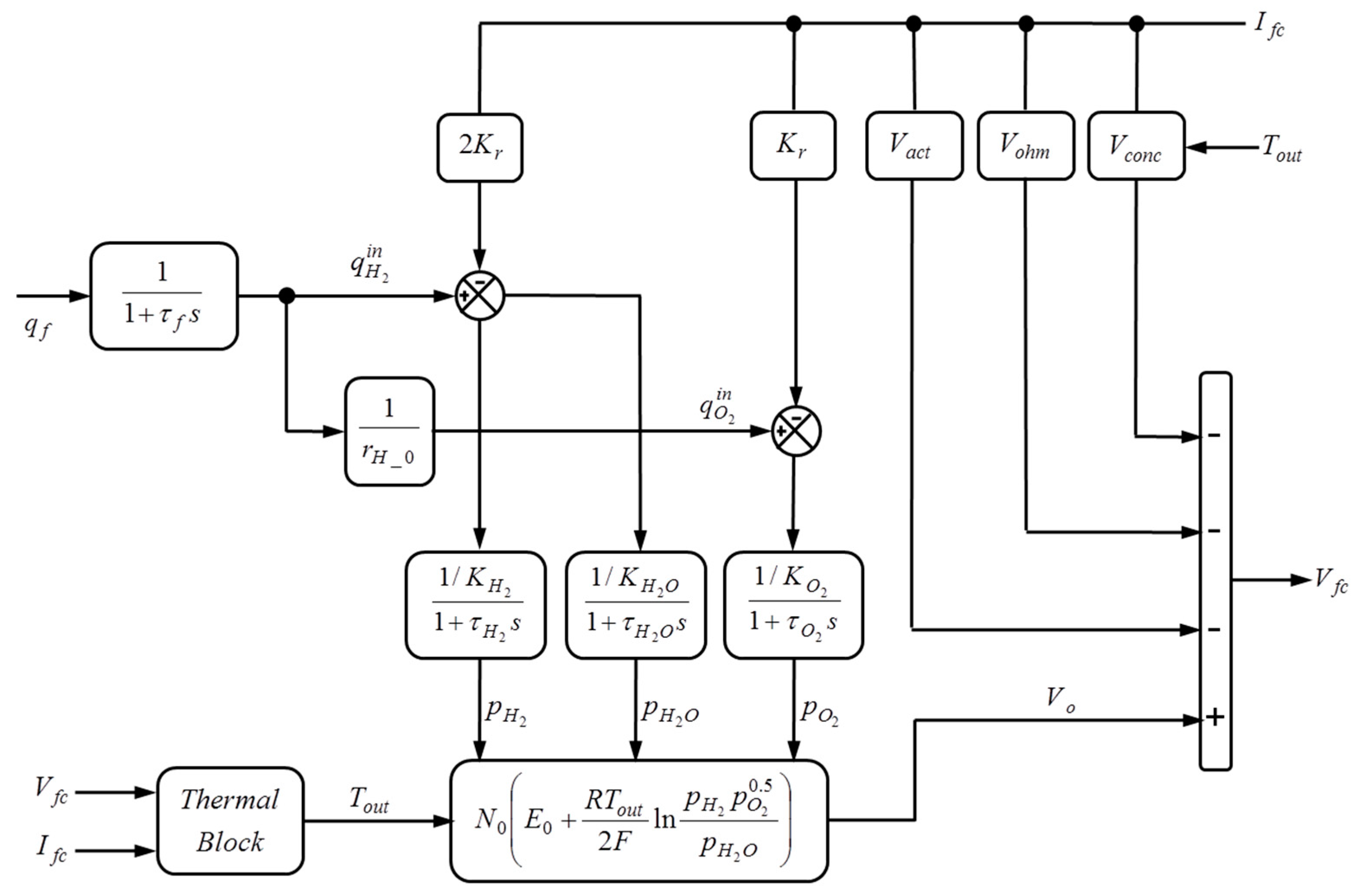
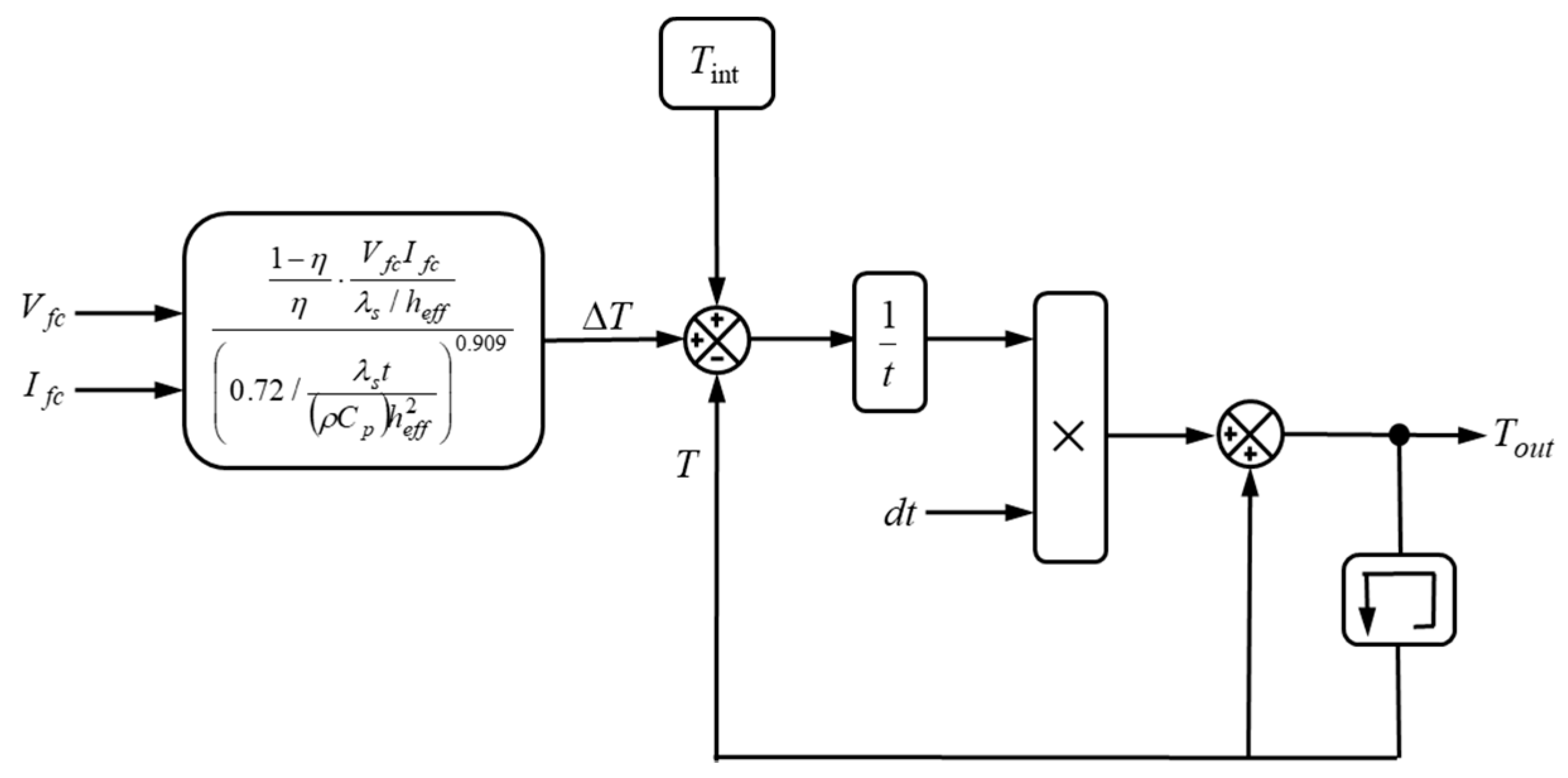
The dynamic model of SOFC we explored in this paper is derived from Reference [22], which is also applied by other scientists in the study of SOFCs [23,24]. This model takes both the electrochemical and the thermal aspects into account. Its structure is shown in Figure 1. Figure 2 shows the detailed structure of the thermal block.

The controlled variable of the system is the output voltage of the SOFC V_fc (V), the manipulate variable of the system is the fuel flow rate q_f (mol/s), while the disturbance variable is the current of the external load I_fc (A). $T_{out}$ is the output temperature, $q_{O_2}^{in}$ (mol/s) is the flow rate of the oxygen, $q_{H_2}$ (mol/s) is the flow rate of the hydrogen, and $p_{H_2}$ (Pa), $p_{H_{2}O}$ (Pa), $p_{O_2}$ (Pa) represent for the partial pressure of the hydrogen, steam, and oxygen, respectively. The other parameters of the model are listed in

Table 1. Nominal parameters of the SOFC system.

Parameter	Representation	Value	Parameter	Representation	Value
$K_r$	Reaction constant	0.993 × 10−3 mol/(s A)	$E_{act}$	Activation energy	120 kJ/mol
$K_{H_2}$	Valve molar constant for hydrogen	0.843 mol/(s atm)	$A$	Pre exponential factor	101.2 kA/cm2
$K_{H_{2}O}$	Valve molar constant for steam	0.281 mol/(s atm)	$\alpha$	Ohmic resistance constant	0.2 Ω
$K_{O_2}$	Valve molar constant for oxygen	2.52 mol/(s atm)	$\beta$	Ohmic resistance constant	−2870 K
${\tau }_{H_2}$	Response time for hydrogen flow	26.1 s	$T_0$	Constant temperature	973 K
${\tau }_{H_{2}O}$	Response time for steam flow	78.3 s	$\eta$	Efficiency	0.8
${\tau }_{O_2}$	Response time for oxygen flow	2.91 s	$h_{eff}$	Thickness	10−3 m
${\tau }_f$	Fuel processor response time	5 s	${\lambda }_s$	Thermal conductivity	2 W/(m K)
$F$	Faraday’s constant	96,486 C/mol	$t$	Relaxation time	200 s
$R$	Gas constant	8.31 J/(mol K)	$\rho$	Density	6600 kg/m3
$E_0$	Ideal standard potential	1.1 V	$c_p$	Heat capacity	400 J/(kg K)
$N$	Number of cells in stack	384	$T_{\mathrm{int}}$	Initial temperature	1273 K

.

The partial pressures can be estimated by the electrochemical relationships as follows [25]:

$$p_{H_2}=\frac{1/K_{H_2}}{1+{\tau }_{H_2}s}\left(\frac{1}{1+{\tau }_{f}s}{q}_f-2K_r{I}_{fc}\right)$$

(1)

$$p_{O_2}=\frac{1/K_{O_2}}{1+{\tau }_{O_2}s}\left(\frac{1/r_{H\_O}}{1+{\tau }_{f}s}{q}_f-K_r{I}_{fc}\right)$$

(2)

$$p_{H_{2}O}=\frac{1/K_{H_{2}O}}{1+{\tau }_{H_{2}O}s}2K_r{I}_{fc}$$

(3)

V₀ (V) is the voltage of the electricity generated by the transport of the electron in the cell, it is calculated with the Nerst’s equation:

$$V_0=N_0\left(E_0+\frac{RT}{2F}\ln \frac{p_{H_2}{p}_{O_2}^{0.5}}{p_{H_{2}O}}\right)$$

(4)

Using the activation loss, concentration loss, and the ohmic loss, the output voltage can be calculated as:

$$V_{fc}=V_o-V_{act}-V_{ohm}-V_{conc}$$

(5)

where V_fc (V) stands for the output voltage of SOFC, V_act (V), V_ohm (V), V_conc (V) is the activation voltage loss, the ohmic voltage loss and the concentration voltage loss, respectively. They can be represented as a function of temperature by the following equations:

$$\begin{array}{c}{V}_{act}=\frac{RT}{F}\left(z+\sqrt{1+z^2}\right)\\ z=I_{fc}/2I_0\\ I_0=A\cdot \exp \left(-E_{act}/RT\right)\end{array}$$

(6)

$$V_{ohm}=\alpha \cdot \exp \left[\beta \left(\frac{1}{T_0}-\frac{1}{T}\right)\right]I_{fc}$$

(7)

$$V_{conc}=\frac{RT}{2F}\ln \left(1-\frac{I_{fc}}{i_L}\right)$$

(8)

where T (°C) denotes the temperature of the fuel cell.

The Fourier number F_o and the source term number S₀ are the two major parameters to demonstrate the thermal equations in a dimensionless form [23]. They are expressed as:

$$F_o=\frac{{\lambda }_{s}t}{\left(\rho c_p\right)h_{eff}^2}$$

(9)

$$S_0=\frac{1-\eta }{\eta }\cdot \frac{V_{fc}{I}_{fc}}{{\lambda }_s\Delta T/h_{eff}}$$

(10)

where t (s) denotes the relaxation time which represents the time for the system to attain 90% of the new steady-state value. $\Delta T$(°C) denotes the temperature change during the period of relaxation time. The relationship between F_o and S₀ can be defined as [23]:

$$F_o=0.72S_0{}^{-1.1}$$

(11)

Based on Equations (9)–(11), the expression of $T_{out}$ can be modified as follow:

$$T_{out}=T+\left(\frac{T_{\mathrm{int}}+\Delta T-T}{t}\right)dt$$

(12)

where T (°C) is the current temperature of the fuel cell, T_int (°C) is the initial temperature of the fuel cell at the time when no load is added, and $dt$ is the step time of Simulink.

Fuel utilization factor u_f is also one of the important indicators of SOFC. It reveals the proportion of the acted fuel flow to the input fuel flow:

$$u_f=\frac{q_{H_2}^{in}-q_{H_2}^{out}}{q_{H_2}^{in}}=\frac{2K_r{I}_{fc}}{q_{H_2}^{in}}$$

(13)

$q_{H_2}^{in}$ in the input of the fuel flow, and $q_{H_2}^{out}$ is the output of the fuel flow. Usually, u_f is constrained to the range of 0.7–0.9 for high efficiency and safety.

2.3. Problem Description

The aim of the control design is to maintain the output voltage to keep up with the rated voltage as accurately as possible, and decrease the voltage variation when the current loads change. The top three problems in control design are listed below:

• Nonlinearity of the System: owning to Nerst’s equation in (4), the SOFC system is characterized as nonlinearity [26], and this deteriorates the control performance of the controller when the working conditions drift off from the ideal working conditions.
• Fuel Flow is Restricted: fuel flow must be restricted between 0 and 2 mol/s, which may cause actuator saturation and the dynamic property may be deteriorated.
• Hysteresis of the System: the rated voltage and the current load change rapidly, while the effect of the fuel flow on the output voltage is comparatively slow.

3. System Identification and Controller Tuning

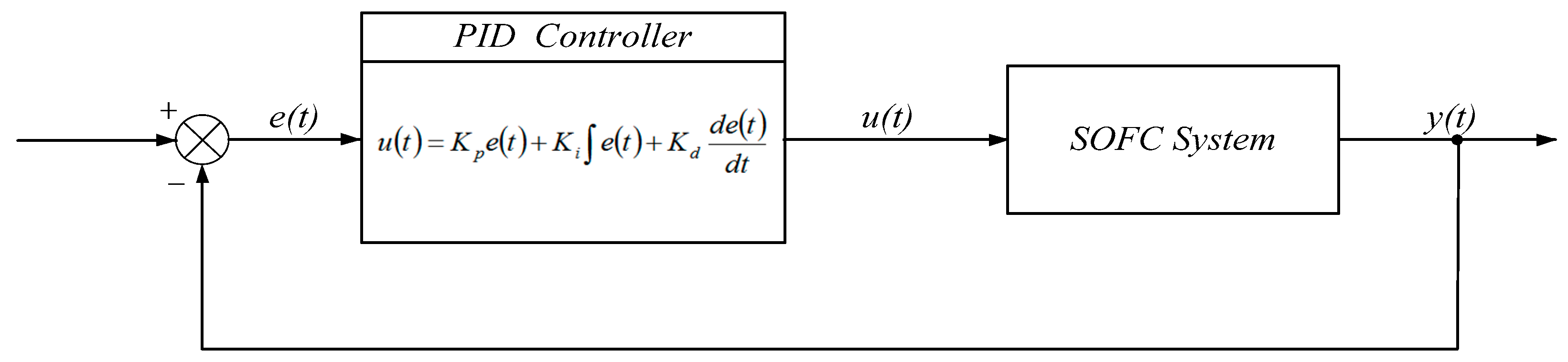
Nowadays, conventional PID controllers are still wildly utilized in the control of industrial process for their high reliability and simplicity [10]. The block diagram of a conventional PID controller is shown in Figure 3. The control equation is given as follows:

$$u\left(t\right)=K_{p}e\left(t\right)+K_i{\displaystyle \int e\left(t\right)+K_d\frac{de\left(t\right)}{dt}}$$

(14)

where $u\left(t\right)$ stands for the control action, K_p, K_i, and K_d are the proportional integral and derivative gains. $e\left(t\right)$ is the tracking error signal.

In this section, we aim to linearize the SOFC model and use the identified model for the purpose of controller tuning. We will use a conventional PID controller to control the SOFC system, and find the parameter of the PID controller with the best step response curve.

3.1. System Identification

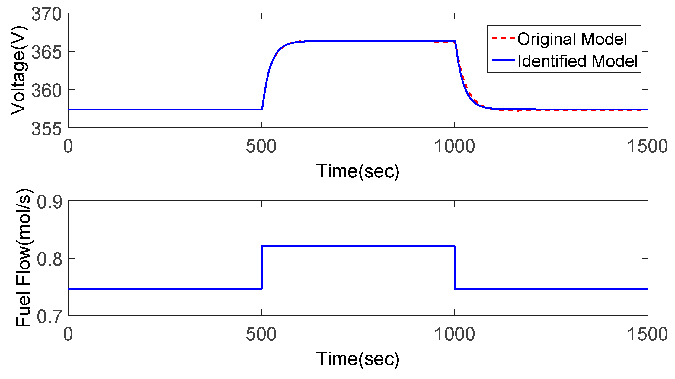
Given that the SOFC model is a nonlinear system, it’s hard to tune the controller with the original model. To get the proper parameter of the PID controller, the first step is to linearize the model. We use the System Identification Toolbox of Matlab to identify the system, and we get the identified model as follows:

$$G\left(s\right)=\frac{2.417s+0.8276}{s^3+0.716s^2+0.1808s+0.006914}$$

(15)

Figure 4 shows the step response of the original model and the identified model. From the response curve, we can tell that the identified model behaves remarkably similar to the original model. Thus, the identification is successful, and we can use the identified model as the linearized model for the controller tuning.

3.2. Controller Tuning

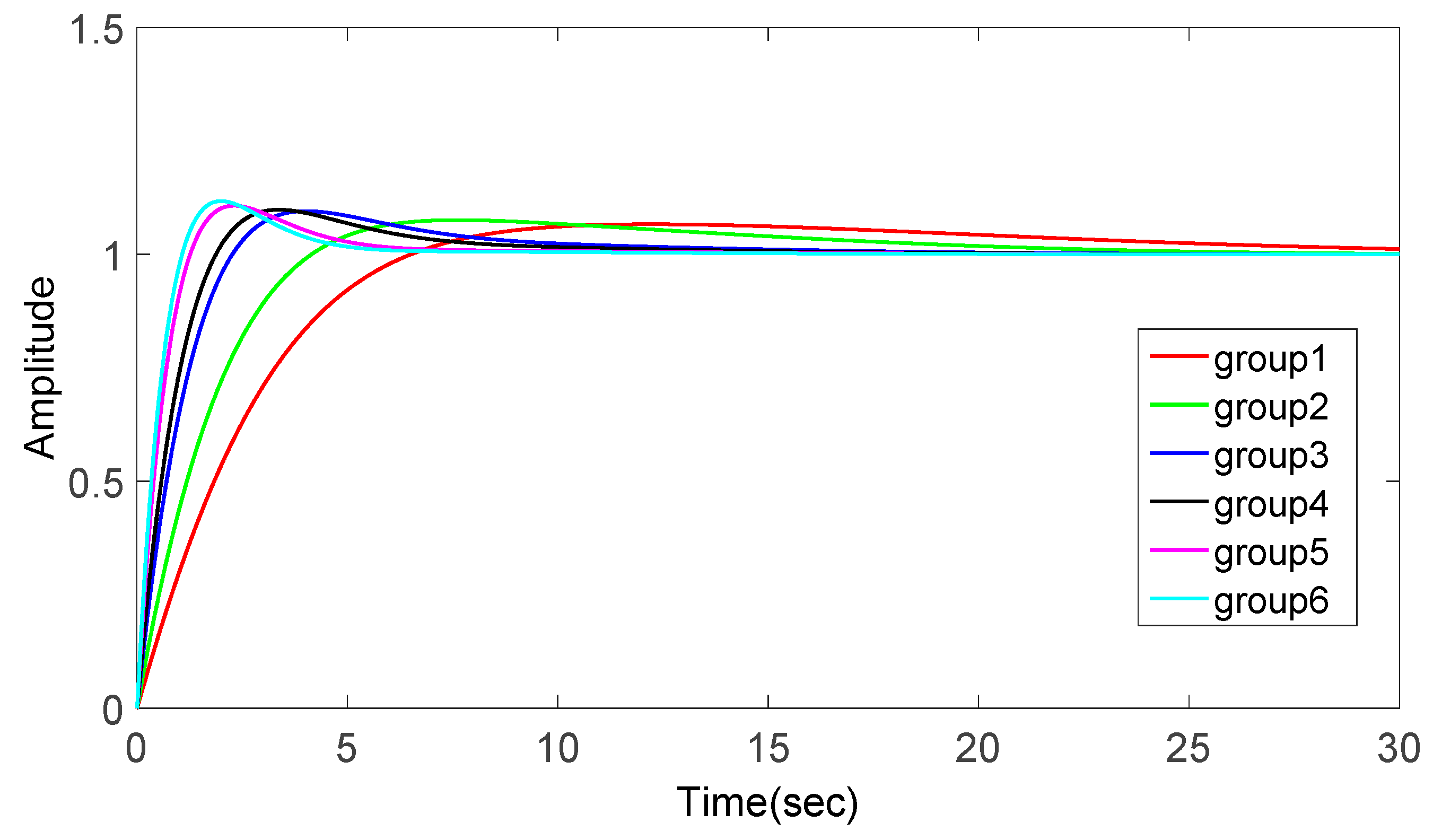
We use the pidTuner Toolbox of Matlab to tune the PID controller and get several groups of proportional, integral, and derivative gains. Then we apply these parameters to the PID controller and record the results of the step response of each group of parameters. The simulation results are shown in Figure 5. It is easy to tell that the overshoot of the output is hard to eliminate with the control of only a conventional PID controller. If the overshoot is slashed excessively, the settling time will be improperly long.

The detailed data of the overshoot and settling time of the step responses are shown in

Table 2. Result of the parameter tuning simulation.

Group	Kp	Ki	Kd	Overshoot (%)	Settling Time (s)
1	0.0722	0.0072	0.1358	6.63	26.5
2	0.1152	0.0145	0.2182	7.62	19.51
3	0.2354	0.0339	0.3628	9.55	13.64
4	0.3022	0.0459	0.4434	9.85	8.81
5	0.5259	0.0824	0.6488	10.72	5.54
6	0.6666	0.1152	0.7475	11.71	4.82

. After synthesizing all of the results, we finally set the parameter of the conventional PID controller as follows to reduce both the overshoot and the settling time:

$$\{\begin{array}{l}{K}_p=0.3314\\ K_i=0.0201\\ K_p=0.4632\end{array}$$

4. Fuzzy Control Design

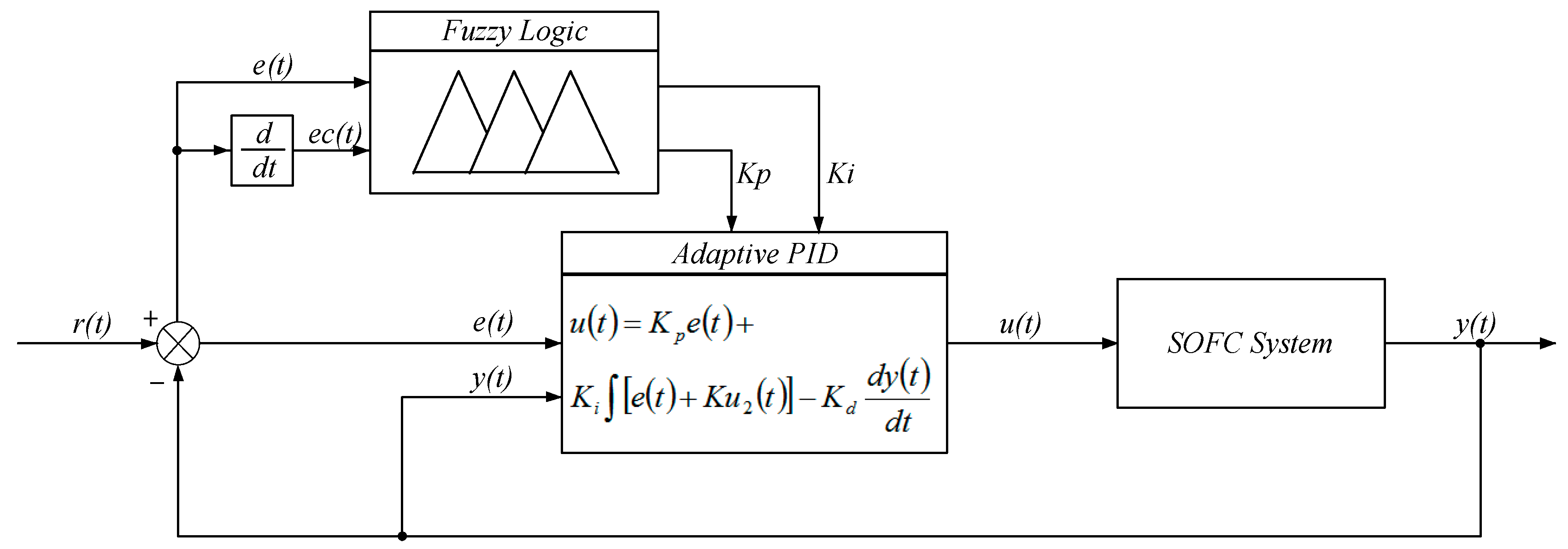
The conventional PID controller is ideal for the control of the linear system. However, due to the nonlinearity of the SOFC system, the control performance will deteriorate with the variation of the working conditions [18]. To this end, we can use PID controllers with variable parameters to overcome the change of the operating point. Based on the variable parameters, the proposed fuzzy adaptive PID controller was designed. The basic block diagram of the system is shown in Figure 6, and the detailed structure of the controller is shown in Figure 7.

The equation of the fuzzy adaptive PID is designed as follows:

$$u\left(t\right)=K_{p}e\left(t\right)+K_i{\displaystyle \int \left[e\left(t\right)+K{u}_2\left(t\right)\right]+K_d\frac{dy\left(t\right)}{t}}$$

(16)

$$u_2\left(t\right)=u_1\left(t\right)-u_0\left(t\right)$$

(17)

where $u\left(t\right)$ stands for the control action, K_p, K_i, and K_d are the proportional integral and derivative gains. $e\left(t\right)$ is the tracking error signal.

4.1. Fuzzy PI Controller

The input of the controller are error e and the change of error, they are given as follows:

$$e\left(k\right)=r\left(k\right)-y\left(k\right)$$

(18)

$$ec\left(k\right)=e\left(k\right)-e\left(k-1\right)$$

(19)

where $r\left(k\right)$ denotes the rated voltage, and $y\left(k\right)$ denotes the output voltage.

The outputs are the modifying value of the proportion gain K_p1 and the modifying value of the integral gain K_i1. The fuzzy controller includes three stages: fuzzification, fuzzy logic judgement, and defuzzification.

4.1.1. Fuzzification

Fuzzification is the process of transforming crisp sets into linguistic fuzzy sets by using fuzzy membership functions. To design the fuzzy logic rule, seven fuzzy items are defined: NB, NM, NS, ZO, PS, PM, and PB, which stands for negative big, negative medium, negative small, zero, positive small, positive medium, and positive big, respectively. The fuzzy membership function of NB and PB are Pi type, while the fuzzy membership function for the rest of the fuzzy items are triangular type. The universe of discourse of e, ec, K_p1 and K_i1 are all [–3, 3], and the gain for e, ec, K_p1 and K_i1 are 0.5, 0.5, 0.1 and 0.04, respectively. The curves are displayed in Figure 8 and Figure 9.

4.1.2. Fuzzy Logic Judgment

The fuzzy logic judgment is the core of fuzzy control which is based on fuzzy logic rules. To design the controller, Mamdani Inference Method [27] was applied for the fuzzy judgment. The output membership value is calculated below:

$${\mu }_{K_{p1}}\left(c_p\right)={\mu }_e(e)\wedge {\mu }_{ec}\left(ec\right)$$

(20)

$${\mu }_{K_{i1}}\left(c_i\right)={\mu }_e\left(e\right)\wedge {\mu }_{ec}\left(ec\right)$$

(21)

where c_p, c_i are the elements in the fuzzy set of K_p1 and K_i1, respectively, and ${\mu }_{Kp1}\left(c_p\right)$, ${\mu }_{Ki1}\left(c_i\right)$ are the membership degrees of c_p and c_i , respectively.

The fuzzy rules are established with 49 items, which are listed in

Table 3. The fuzzy logic rules of the controller.

Kp1/Ki1	ec	NB	NM	NS	ZO	PS	PM	PB
e
NB		PB/NB	PB/NB	PM/NM	PM/NM	PS/NS	ZO/ZO	ZO/ZO
NM		PB/NB	PB/NB	PM/NM	PS/NS	PS/NS	ZO/ZO	NS/ZO
NS		PM/NB	PM/NM	PM/NS	PS/NS	ZO/ZO	NS/PS	NS/PS
ZO		PM/NM	PM/NM	PS/NS	ZO/ZO	NS/PS	NM/PM	NM/PM
PS		PS/NM	PS/NS	ZO/ZO	NS/PS	NS/PS	NM/PM	NM/PB
PM		PS/ZO	ZO/ZO	NS/PS	NM/PS	NM/PM	NM/PB	NB/PB
PB		ZO/ZO	ZO/ZO	NM/PS	NM/PM	NM/PM	NB/PB	NB/PB

. The rules can be expressed as “ If e is A_i and ec is B_i, then K_p1 is C_i and K_i1 is D_i”, where A_i, B_i, C_i and D_i are the fuzzy items of the universe of discourse of e, ec, K_p1 and K_i1, respectively.

4.1.3. Defuzzification

In the process of defuzzification, the weighted mean was utilized to convert the vector into a single value [28], and then the output of the fuzzy controller was determined.

The calculation of K_p1 and K_i1 are below:

$$K_{p1}=\frac{{\sum }_{i=1}^m{\mu }_{K_{p1i}}\left(c_p\right)\cdot c_{pi}}{{\sum }_{i=1}^m{\mu }_{K_{p1i}}\left(c_p\right)}$$

(22)

$$K_{i1}=\frac{{\sum }_{j=1}^n{\mu }_{K_{i1j}}\left(c_i\right)\cdot c_{ij}}{{\sum }_{j=1}^n{\mu }_{K_{i1j}}\left(c_i\right)}$$

(23)

With the output of the Fuzzy controller, the proportion gain K_p and the integral gain K_i can be calculated as follows:

$$K_p=K_{p0}+K_1\cdot K_{p1}$$

(24)

$$K_i=K_{i0}+K_2\cdot K_{i1}$$

(25)

where K_p0 is the initial value of the proportion gain, K_i0 is the initial value of the integral gain, K₁ and K₂ are both constant which denotes the gain of K_p1 and K_i1, respectively.

4.2. The Realization of Anti-Windup

In this paper, the fuel flow rate is limited to between 0 and 2 mol/s. Due to this limitation, there might be the problem of actuator saturation. To this end, a method based on back-calculation is applied [19]. As shown in Figure 7, a feedback for the integrator is designed. The input of the integrator can be calculated as:

$$e_1(t)=e_0(t)+K\cdot u_2(t)$$

(26)

where $e_1\left(t\right)$ denotes the input of the integrator, $e_0\left(t\right)$ denotes the tracking error signal, $u_0\left(t\right)$, and $u_1\left(t\right)$ denotes the controlled signal before and after the saturation block, respectively. $u_2\left(t\right)$ is the difference between $u_1\left(t\right)$ and $u_0\left(t\right)$ as (17) shows.

From Equations (17) and (26), we can tell that when the controlled signal is above the upper limit, $u_1\left(t\right)$ will remain the upper limit, and $u_1\left(t\right)$ will be smaller than $u_0\left(t\right)$. This will set $u_2\left(t\right)$ as a negative signal to reduce the integral action. On the contrary, when the controlled signal is under the lower limit, $u_1\left(t\right)$ will remain the lower limit, and $u_1\left(t\right)$ will be bigger than $u_0\left(t\right)$. This will set $u_2\left(t\right)$ as a positive signal to increase the integral action. In this way, the controller is able to get rid of the situation of actuator saturation much faster and reduce the overshoot at the same time.

4.3. Differential Forward Algorithm

Owning to the fact that the differentiator is very sensitive to the variation of the input [20], the proposed controller applies a differential forward algorithm to overcome the sensibility of the differentiator. In the conventional PID, the controller differentiates to the tracking error signal $e\left(t\right)$, which is defined in (14). As we can see, when the rated voltage $r\left(t\right)$ changes, the output voltage $y\left(t\right)$ still remains the same, which causes a sudden variation of $e\left(t\right)$. This will lead to a “snap back” of the differential action.

On the contrary, the differential forward algorithm differentiates to the output voltage $y\left(t\right)$ directly. Meanwhile, the differentiator applies the first order actual differential algorithm, which can be expressed as:

$$G_D\left(s\right)=\frac{s}{0.1s+1}$$

(27)

In this way, the variation of the rated voltage is not able to affect the differentiator, and because the output voltage has a relatively slow rate of change, it will not produce a large control value. With this method, the problem of the “snap back” of the differential action is fixed.

5. Simulation

In this section, to show the comparison of the robustness of the proposed controller and the conventional PID controller, simulation of step response and disturbance response based on the tuned PID controller in Section 3.2 and the proposed controller in Section 4 is implemented, and the results of the simulation are displayed.

5.1. Simulation of Step Response

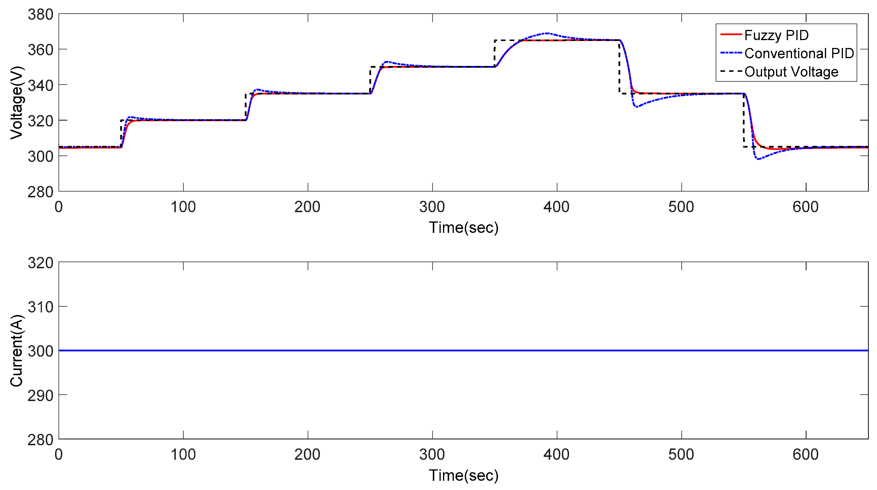
During the process of step response, the current is kept at 300 A, the rated voltage begins with 305 V, and then it is set to increase by 15 V at 50 s, 150 s, 250 s, and 350 s. Then the rated voltage decreases by 30 V at 450 s and 550 s to return to 305 V. The results of the simulation are shown in Figure 10.

The detailed data of the simulation result are displayed in

Table 4. Detailed data of the simulation result of step response.

Conventional PID				Fuzzy PID
Number	Overshoot (%)	Settling Time (s)	Saturation Time (s)	Number	Overshoot (%)	Settling Time (s)	Saturation Time (s)
1	0.56	30.85	1.58	1	0	9.28	0.53
2	0.66	34.72	3.10	2	0	10.41	2.29
3	0.83	42.91	7.62	3	0	12.23	6.71
4	1.68	78.53	38.55	4	0	22.21	20.04
5	−2.09	62.78	9.63	5	0	18.52	8.62
6	−2.26	57.91	6.72	6	0	20.56	4.68

.

As we can tell from the results, the control performance of the PID controller deteriorates with the variation of the working conditions, which is illustrated by the increase of the overshoot and the settling time. As for the proposed controller, the overshoot keeps at 0 for all the working conditions, and the settling time is also much shorter than the conventional PID controller. Meanwhile, with the design of anti-windup structure, there is also a reduction in the saturation time. Especially in working condition 4, the saturation time of the conventional PID controller is two times bigger than the proposed controller.

5.2. Simulation of Disturbance Response

During the process of disturbance response, the rated voltage is kept at 305 V, and the current starts with 300 A, then the current is set to increase by 75 A at 50 s, 100 s, 150 s, and 200 s and then decreases by 150 A at 250 s and 300 s to return to 300 A. The results of the simulation are shown in Figure 11.

The detailed data of the simulation result are displayed in

Table 5. Detailed data of the simulation result of disturbance response.

Conventional PID				Fuzzy PID
Number	Overshoot (%)	Settling Time (s)	Saturation Time (s)	Number	Overshoot (%)	Settling Time (s)	Saturation Time (s)
1	0.33	23.28	1.51	1	0	12.14	1.13
2	0.43	26.02	2.61	2	0	12.71	2.98
3	0.59	30.29	5.23	3	0	13.07	5.09
4	0.82	34.31	12.94	4	0	15.13	9.87
5	−0.79	37.63	5.03	5	0	13.67	5.47
6	−1.11	39.42	5.65	6	0	14.45	5.32

.

Similar to the result of step response, the proposed controller shows a better control performance in the control of disturbance response. To illustrate, with the variation of the working condition, the absolute value of the overshoot of the conventional PID controller varies from 0.33 to 1.11, and the overshoot is kept at 0 for the proposed controller. The settling time of the proposed controller is much shorter than the conventional PID controller. In addition, the average of the saturation time of the proposed controller is also shorter than the conventional PID controller. In working condition 4, especially, the saturation time of the proposed controller is three quarters of the saturation time of conventional PID controller.

5.3. Discussion

From the simulation results, we can tell that the proposed controller has the advantage of no overshoot, less settling time, and less saturation time. Under the shifting working conditions, the working performance of the PID controller deteriorates significantly, while the proposed controller is less affected and performs much better than the conventional PID controller.

In conclusion, the proposed controller is able to handle the nonlinearity of SOFC, and it is expected to be an efficient solution for the problem of controlling the output voltage of SOFCs.

6. Conclusions

The nonlinearity, slow dynamics, and limited constraint make the voltage regulation of SOFCs challenging and adds to the difficulty of the utilization of SOFCs. Inspired by the application of fuzzy control on nonlinearity systems and the advantages of PID controller, this paper designed a fuzzy adaptive PID controller for voltage regulation of SOFCs. With the effect of the fuzzy controller, the parameters of the PID controller coordinate with the change in the working conditions, which overcomes the nonlinearity of SOFCs and brings a better control performance. At the same time, the back-calculating method based on an anti-windup structure enables the controller to shorten the saturation time of the actuators and reduce the overshoot. In addition, the differential forward algorithm was applied to help the controller reduce the “snap back” phenomenon of the derivative action and improve the robustness of the controller at the same time. The simulation results in Section 5 illustrate that a fuzzy adaptive PID control has the advantages of (1) no overshoot; (2) less settling time; (3) no oscillation, and (4) less saturation time. Compared to the conventional PID controller, the proposed controller has a more robust control property for the change of the rated voltage and current disturbance, and possesses a better control performance. With these characteristics, the proposed controller can be an ideal alternative for the control of SOFCs.

References

- O’Hayre, R.P. Fuel cells for electrochemical energy conversion. EPJ Web Conf. 2017, 148, 1–16. [Google Scholar] [CrossRef]
- Ormerod, R.M. Solid Oxide Fuel Cells. Chem. Soc. Rev. 2003, 34, 17–28. [Google Scholar] [CrossRef]
- Thattai, A.T.; Oldenbroek, V.; Schoenmakers, L.; Woudstra, T.; Aravind, P.V. Research Paper: Towards retrofitting integrated gasification combined cycle (IGCC) power plants with solid oxide fuel cells (SOFC) and CO2 capture—A thermodynamic case study. Appl. Therm. Eng. 2017, 114, 170–185. [Google Scholar] [CrossRef]
- Das, V.; Padmanaban, S.; Venkitusamy, K.; Selvamuthukumaran, R.; Blaabjerg, F.; Siano, P. Recent advances and challenges of fuel cell based power system architectures and control—A review. Renew. Sustain. Energy Rev. 2017, 73, 10–18. [Google Scholar] [CrossRef]
- Ogawa, T.; Takeuchi, M.; Kajikawa, Y. Comprehensive Analysis of Trends and Emerging Technologies in All Types of Fuel Cells Based on a Computational Method. Sustainability 2018, 10, 458. [Google Scholar] [CrossRef]
- Stambouli, A.B.; Traversa, E. Solid oxide fuel cells (SOFCs): A review of an environmentally clean and efficient source of energy. Renew. Sustain. Energy Rev. 2002, 6, 433–455. [Google Scholar] [CrossRef]
- Knyazkin, V.; Söder, L.; Canizares, C. Control challenges of fuel cell-driven distributed generation. In Proceedings of the 2003 IEEE Bologna Power Tech Conference Proceedings, Bologna, Italy, 23–26 June 2003; Volume 2, p. 2. [Google Scholar]
- Sun, L.; Hua, Q.; Shen, J.; Xue, Y.; Li, D.; Lee, K.Y. A Combined Voltage Control Strategy for Fuel Cell. Sustainability 2017, 9, 1517. [Google Scholar] [CrossRef]
- Sun, L.; Hua, Q.; Shen, J.; Xue, Y.; Li, D.; Lee, K.Y. Multi-objective optimization for advanced superheater steam temperature control in a 300 MW power plant. Appl. Energy 2017, 208, 592–606. [Google Scholar] [CrossRef]
- Sun, L.; Li, D.; Lee, K.Y. Optimal disturbance rejection for PI controller with constraints on relative delay margin. ISA Trans. 2016, 63, 103–111. [Google Scholar] [CrossRef] [PubMed]
- Li, Y.H.; Choi, S.S.; Rajakaruna, S. An analysis of the control and operation of a solid oxide fuel-cell power plant in an isolated system. IEEE Trans. Energy Convers. 2005, 20, 381–387. [Google Scholar] [CrossRef]
- Lesnicar, A.; Marquardt, R. An innovative modular multilevel converter topology suitable for a wide power range. In Proceedings of the 2003 IEEE Bologna Power Tech Conference Proceedings, Bologna, Italy, 23–26 June 2003. [Google Scholar]
- Razbani, O.; Assadi, M. Artificial neural network model of a short stack solid oxide fuel cell based on experimental data. J. Power Sources 2014, 246, 581–586. [Google Scholar] [CrossRef]
- Chettibi, N.; Mellit, A.; Sulligoi, G.; Massi Pavan, A. Fuzzy-based power control for distributed generators based on solid oxide fuel cells. In Proceedings of the 2015 International Conference on Clean Electrical Power (ICCEP), Taormina, Italy, 16–18 June 2015. [Google Scholar]
- Huo, H.B.; Zhu, X.J.; Hu, W.Q.; Tu, H.Y.; Li, J.; Yang, J. Nonlinear model predictive control of SOFC based on a Hammerstein model. J. Power Sources 2008, 185, 338–344. [Google Scholar] [CrossRef]
- Benchouia, N.E.; Derghal, A.; Mahmah, B.; Madi, B.; Khochemane, L.; Aoul, E.H. An adaptive fuzzy logic controller (AFLC) for PEMFC fuel cell. Int. J. Hydrog. Energy 2015, 40, 13806–13819. [Google Scholar] [CrossRef]
- Kisacikoglu, M.C.; Uzunoglu, M.; Alam, M.S. Fuzzy Logic Control of a Fuel Cell/Battery/Ultra-capacitor Hybrid Vehicular Power System. In Proceedings of the 2007 IEEE Vehicle Power and Propulsion Conference, Arlington, TX, USA, 9–12 September 2007; p. 591. [Google Scholar]
- Van, T.L.; Nguyen, T.H.; Lee, D.C. Advanced Pitch Angle Control Based on Fuzzy Logic for Variable-Speed Wind Turbine Systems. IEEE Trans. Energy Convers. 2015, 30, 578–587. [Google Scholar] [CrossRef]
- Galeani, S.; Tarbouriech, S.; Turner, M.; Zaccarian, L. A Tutorial on Modern Anti-windup Design. Eur. J. Control 2009, 15, 418–440. [Google Scholar] [CrossRef]
- Zhang, H.; Li, Z. Simulation of networked control system based on Smith compensator and single neuron incomplete differential forward PID. J. Netw. 2011, 6, 1675–1681. [Google Scholar] [CrossRef]
- Mahato, N.; Banerjee, A.; Gupta, A.; Omar, S.; Balani, K. Progress in material selection for solid oxide fuel cell technology: A review. Prog. Mater. Sci. 2015, 72, 141–337. [Google Scholar] [CrossRef]
- Achenbach, E. Response of a solid oxide fuel cell to load change. J. Power Sources 1995, 57, 105–109. [Google Scholar] [CrossRef]
- Wu, G.; Sun, L.; Lee, K.Y. Disturbance rejection control of a fuel cell power plant in a grid-connected system. Control Eng. Pract. 2017, 60, 183–192. [Google Scholar] [CrossRef]
- Sedghisigarchi, K.; Feliachi, A. Dynamic and transient analysis of power distribution systems with fuel Cells-part I: Fuel-cell dynamic model. IEEE Trans. Energy Convers. 2004, 19, 423–428. [Google Scholar] [CrossRef]
- Padulles, J.; Ault, G.W.; McDonald, J.R. An integrated SOFC plant dynamic model for power systems simulation. J. Power Sources 2000, 86, 495–500. [Google Scholar] [CrossRef]
- Sun, L.; Li, D.; Wu, G.; Lee, K.Y.; Xue, Y. A Practical Compound Controller Design for Solid Oxide Fuel Cells. IFAC PapersOnLine 2015, 48, 445–449. [Google Scholar] [CrossRef]
- Jayakumar, A.; Ramos, M.; Al-Jumaily, A. A novel fuzzy schema to control the temperature and humidification of PEM fuel cell system. Am. Soc. Mech. Eng. 2015. [Google Scholar] [CrossRef]
- Li, Q.; Chen, W.; Liu, Z.; Li, M.; Ma, L. Development of energy management system based on a power sharing strategy for a fuel cell-battery-supercapacitor hybrid tramway. J. Power Sources 2015, 279, 267–280. [Google Scholar] [CrossRef]
Figure 1.
The block diagram of the dynamic model of the solid oxide fuel cell (SOFC).
Figure 2.
The block diagram of the thermal block of the SOFC.
Figure 3.
Block diagram of the conventional proportional-integral-derivative (PID) controller.
Figure 4.
Comparison of the step response of the original model and the identified model.
Figure 5.
Step response of the identified model.
Figure 6.
Block diagram of the fuzzy adaptive PID controller.
Figure 7.
Detailed structure of the proposed controller.
Figure 8.
Membership function of the input of fuzzy PID: (a) input with e; (b) input with ec.
Figure 9.
Membership function of the output of fuzzy PID: (a) output with Kp1; (b) output with Ki1.
Figure 10.
Simulation result of step response.
Figure 11.
Simulation result of disturbance response.