Nonlinear Error Propagation Analysis of a New Family of Model-Based Integration Algorithm for Pseudodynamic Tests

Abstract
:1. Introduction
2. A New Family of Model-Based Integration Algorithm
3. Pseudodynamic Test Procedure
4. Derivation of Error Propagation Equation
5. Examples for Error Propagation Effect
6. Numerical Simulation of Pseudodynamic Testing
7. Conclusions
- (1)
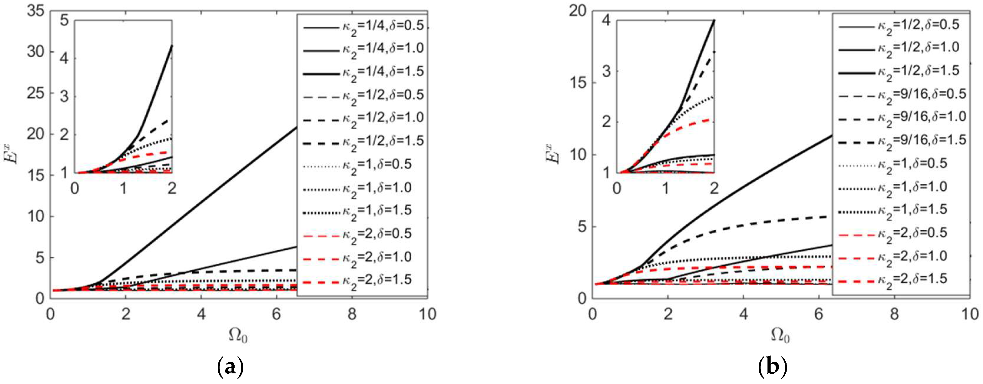
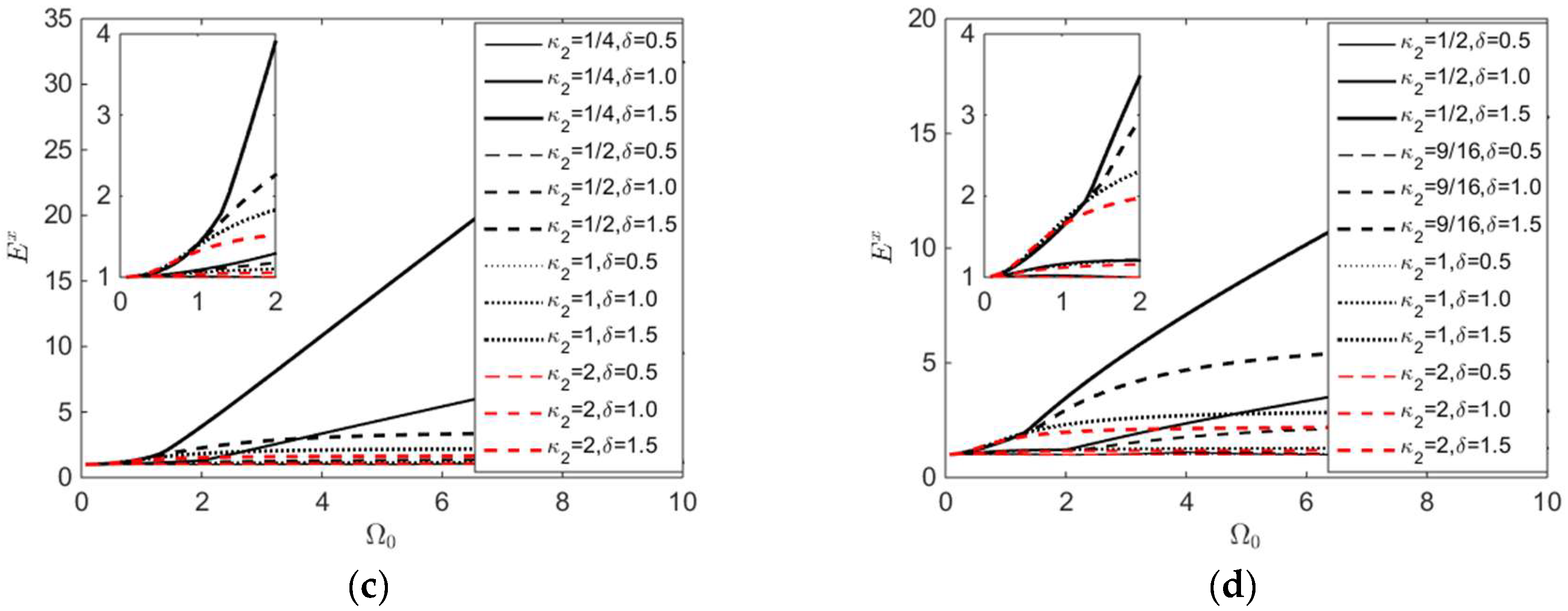
- Both amplification error factors, i.e., and , increase with .
- (2)
- Both amplification factors, i.e., and , increase with the degree of nonlinearity δ, so it is crucial to take the degree of nonlinearity δ into consideration.
- (3)
- As for the viscous damping, it has a positive effect on reducing the errors, so it is conservative to ignore the influence of viscous damping.
- (4)
- Both the two additional coefficients, i.e., and , of the GCR algorithms have great impact on the error propagation property. With the increasing of , the errors increase, while both amplification factors and increasing with the decrease of .
- (5)
- The original CR algorithm with has a relatively large error propagation property, especially for the nonlinear structures with stiffness hardening. The two amplification error factors, i.e., and , of the GCR algorithm with are only 10.8% and 4.6% of those of the original CR algorithm with when for the nonlinear structure with stiffness hardening of Case 3 without viscous damping. Therefore, the GCR algorithm with is a superior alternative of the original CR algorithm with .
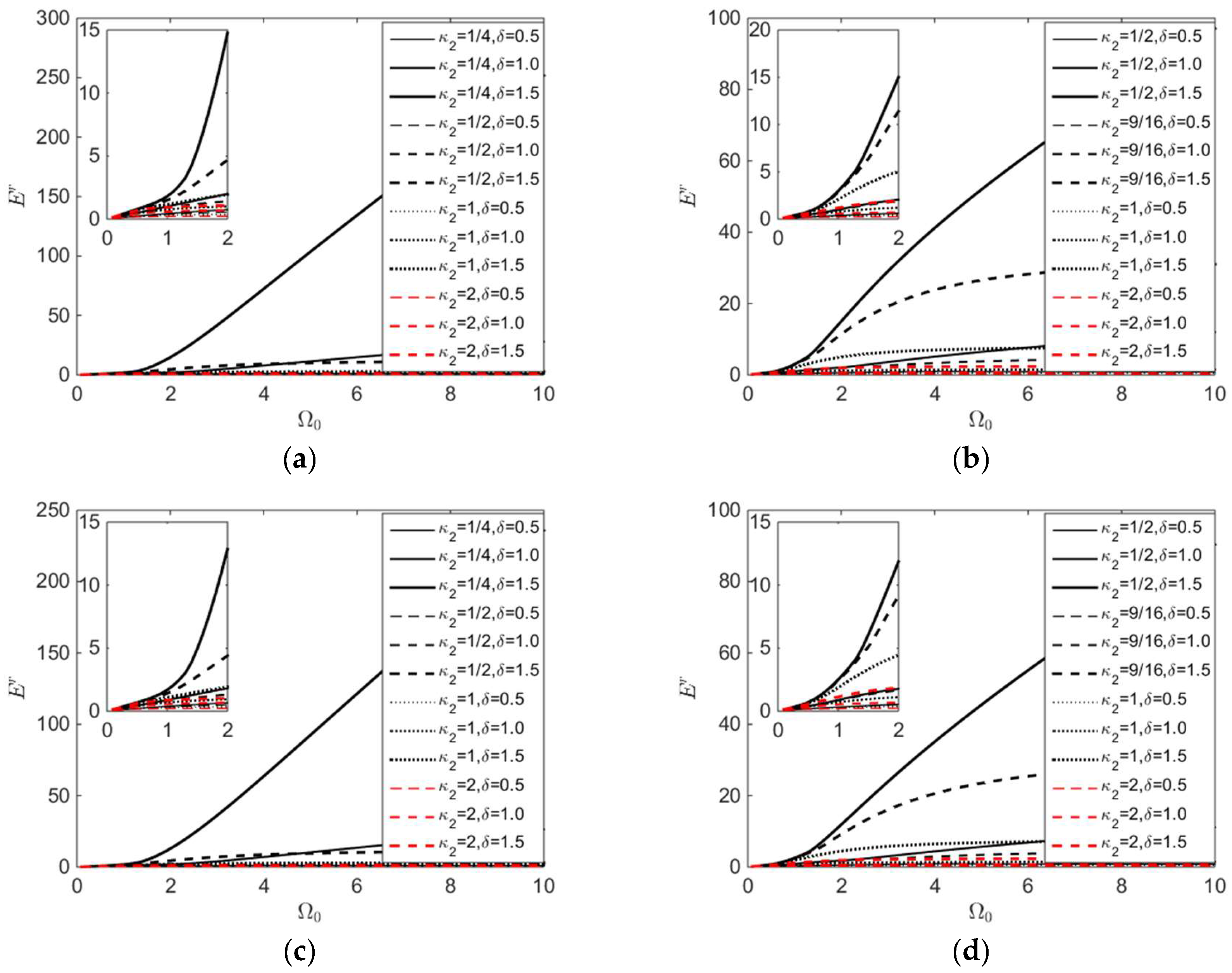
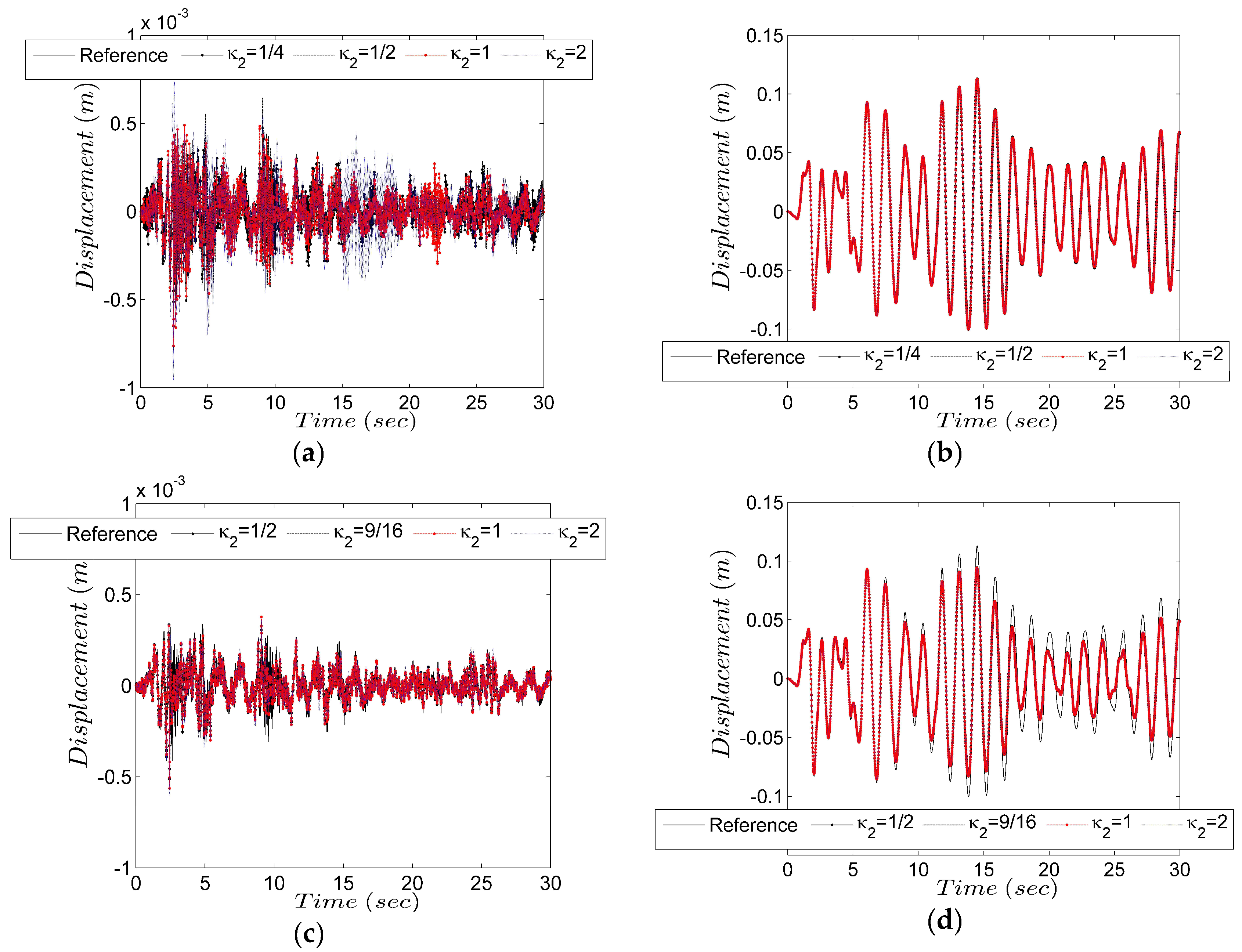
- (6)
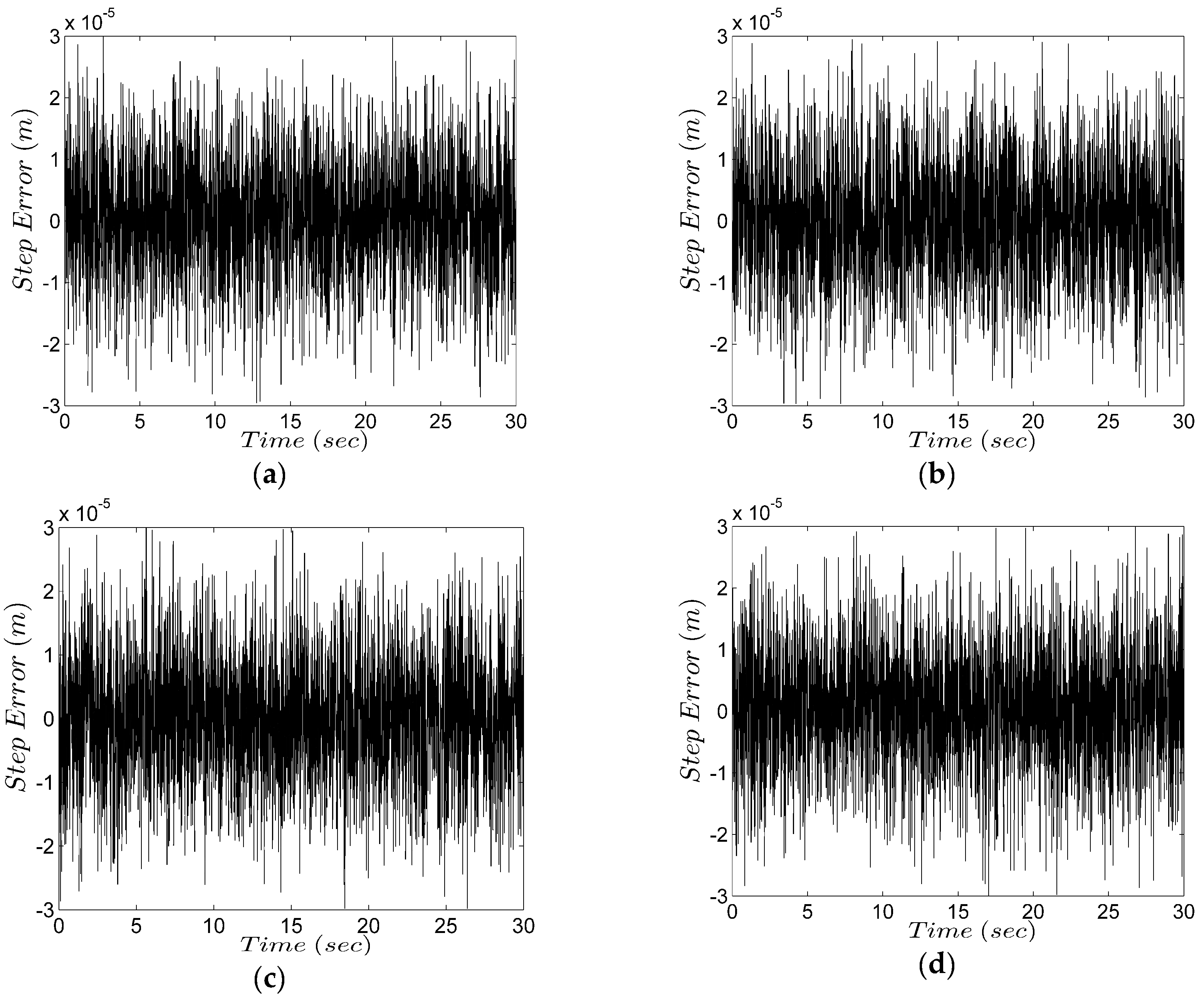
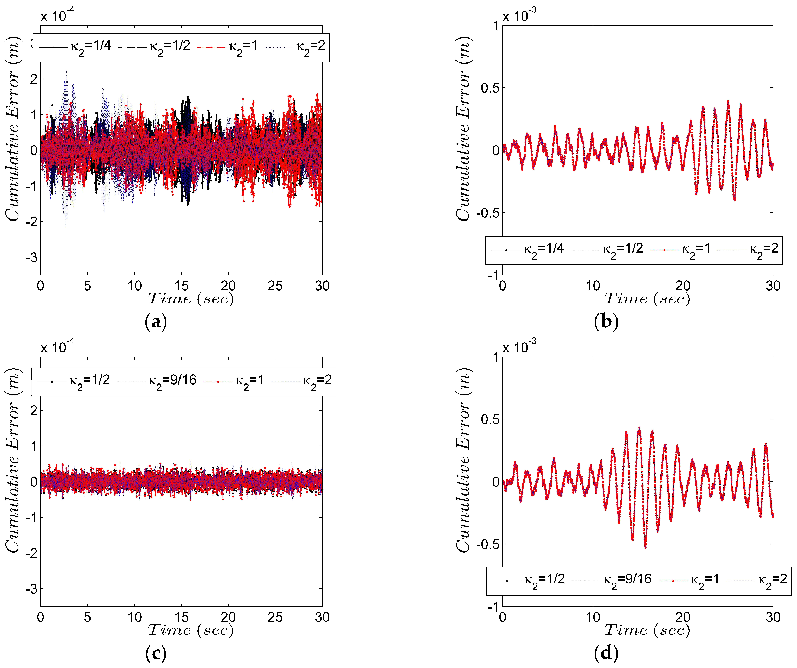
- The displacement response at the first story is significantly disturbed by the error, whereas the influence of error on the displacement response at the second story is inconspicuous. The main reason is that the displacement at the second story is mainly contributed by the first order modal response, while the displacement at the first story is, to some extent, contributed by the second modal response.
- (7)
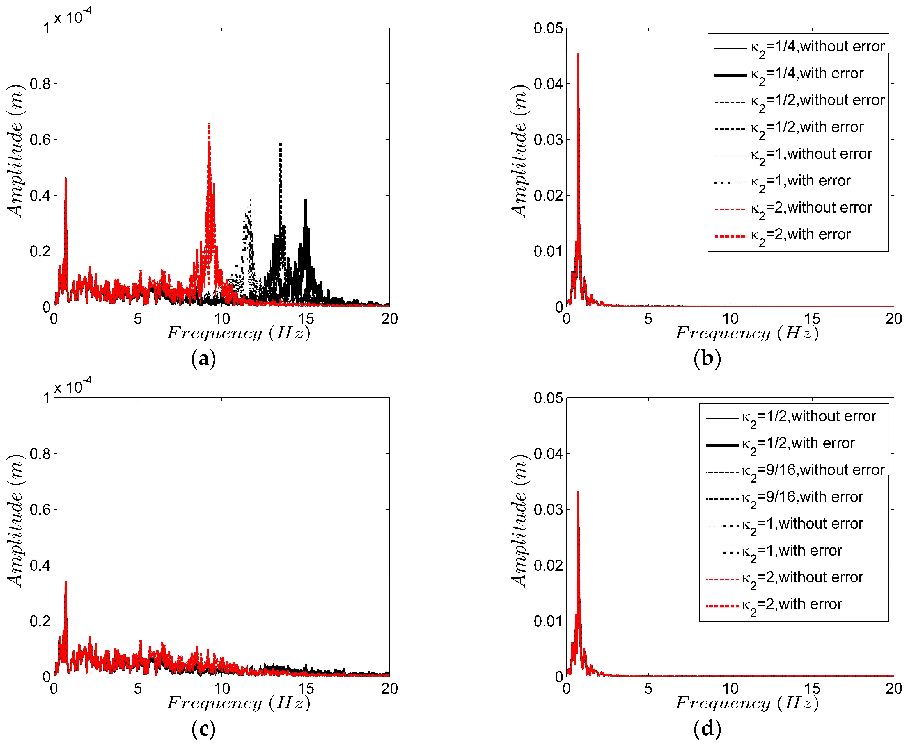
- The maximum displacement at the second story obtained by using the GCR algorithms with are 83% of the reference value. It means that the accuracy of the numerical result is impaired by excessive numerical damping for the high frequency response, thus the numerical dissipation characteristics of the GCR algorithms should be optimized in the future.
Author Contributions
Funding
Conflicts of Interest
Appendix A: Notations
Appendix B

References
- Takanashi, K.; Udagawa, K.; Seki, M.; Okada, T.; Tanaka, H. Nonlinear Earthquake Response Analysis of Structures by a Computer-Actuator On-Line System; University of Tokyo: Tokyo, Japan, 1975. [Google Scholar]
- Abbiati, G.; Bursi, O.S.; Caperan, P.; Di Sarno, L.; Molina, F.J.; Paolacci, F.; Pegon, P. Hybrid simulations of a multi-span RC viaduct with plain bars and sliding bearings. Earthq. Eng. Struct. Dyn. 2015, 44, 2221–2240. [Google Scholar] [CrossRef]
- Elnashai, A.S.; Di Sarno, L. Fundamentals of Earthquake Engineering; Wiley and Sons: Chichester, UK 2008. [Google Scholar]
- Chang, S.Y. Explicit pseudodynamic algorithm with unconditional stability. J. Eng. Mech. 2002, 128, 935–947. [Google Scholar] [CrossRef]
- Chen, C.; Ricles, J.M. Development of direct integration algorithms for structural dynamics using discrete control theory. J. Eng. Mech. 2008, 134, 676–683. [Google Scholar] [CrossRef]
- Kolay, C.; Ricles, J.M. Development of a family of unconditionally stable explicit direct integration algorithms with controllable numerical energy dissipation. Earthq. Eng. Struct. Dyn. 2014, 43, 1361–1380. [Google Scholar] [CrossRef]
- Kolay, C.; Ricles, J.M. Assessment of explicit and semi-explicit classes of model-based algorithms for direct integration in structural dynamics. Int. J. Numer. Methods Eng. 2016, 107, 49–73. [Google Scholar] [CrossRef]
- Peek, R.; Yi, W.H. Error analysis for pseudodynamic test method. I: Analysis. J. Eng. Mech. 1990, 116, 1618–1637. [Google Scholar] [CrossRef]
- Peek, R.; Yi, W.H. Error analysis for pseudodynamic test method. II: Application. J. Eng. Mech. 1990, 116, 1638–1658. [Google Scholar] [CrossRef]
- Shing, P.B.; Mahin, S.A. Cumulative experimental errors in pseudodynamic tests. Earthq. Eng. Struct. Dyn. 1987, 15, 409–424. [Google Scholar] [CrossRef]
- Shing, P.B.; Mahin, S.A. Experimental error effects in pseudodynamic testing. J. Eng. Mech. 1990, 116, 805–821. [Google Scholar] [CrossRef]
- Shing, P.B.; Manivannan, T. On the accuracy of an implicit algorithm for pseudodynamic tests. Earthq. Eng. Struct. Dyn. 1990, 19, 631–651. [Google Scholar] [CrossRef]
- Chang, S.Y. Nonlinear error propagation analysis for explicit pseudodynamic algorithm. J. Eng. Mech. 2003, 129, 841–850. [Google Scholar] [CrossRef]
- Chang, S.Y. Error propagation of HHT-α method for pseudodynamic tests. J. Earthq. Eng. 2005, 9, 223–246. [Google Scholar] [CrossRef]
- Chang, S.Y. Error propagation in implicit pseudodynamic testing of nonlinear systems. J. Eng. Mech. 2005, 131, 1257–1269. [Google Scholar] [CrossRef]
- Bousias, S.; Sextos, A.; Kwon, O.H.; Taskari, O.; Elnashai, A.S.; Evangeliou, N.; Di Sarno, L. Intercontinental hybrid simulation for the assessment of a three-span R/C highway overpass. J. Earthq. Eng. 2017. [Google Scholar] [CrossRef]
- Fu, B. Substructure Shaking Table Testing Method Using Model-Based Integration Algorithms. Ph.D. Thesis, Tongji University, Shanghai, China, 2017. (In Chinese). [Google Scholar]
- MATLAB. Version 2014a; The MathWorks Inc.: Natick, MA, USA, 2014.
- Chopra, A.K. Dynamic of Structures: Theory and Applications to Earthquake Engineering, 4th ed.; Prentice Hall: Upper Saddle River, NJ, USA, 2012. [Google Scholar]
- Chang, S.Y. The γ-function pseudodymamic algorithm. J. Earthq. Eng. 2000, 4, 303–320. [Google Scholar] [CrossRef]


© 2018 by the authors. Licensee MDPI, Basel, Switzerland. This article is an open access article distributed under the terms and conditions of the Creative Commons Attribution (CC BY) license (http://creativecommons.org/licenses/by/4.0/).
Share and Cite
Fu, B.; Jiang, H.; Wu, T. Nonlinear Error Propagation Analysis of a New Family of Model-Based Integration Algorithm for Pseudodynamic Tests. Sustainability 2018, 10, 2846. https://doi.org/10.3390/su10082846
Fu B, Jiang H, Wu T. Nonlinear Error Propagation Analysis of a New Family of Model-Based Integration Algorithm for Pseudodynamic Tests. Sustainability. 2018; 10(8):2846. https://doi.org/10.3390/su10082846
Chicago/Turabian StyleFu, Bo, Huanjun Jiang, and Tao Wu. 2018. "Nonlinear Error Propagation Analysis of a New Family of Model-Based Integration Algorithm for Pseudodynamic Tests" Sustainability 10, no. 8: 2846. https://doi.org/10.3390/su10082846