Carbon Emissions Cost Analysis with Activity-Based Costing

Abstract

Due to growing awareness about environmental issues, consumers are becoming more likely to purchase environmentally friendly products that involve lower carbon emissions (CE). Environmental regulations are being enforced and lower-carbon products are being produced in order to maintain competitiveness when complying with such regulations. This paper aims to explore the effect of CE on profit through three kinds of models using the activity-based costing (ABC) approach. The results indicate that governmental policy makers can effectively decrease CE by Total Quantity Control (TQC) to resolve problems of environmental degradation. Governmental policy makers can control CE by limiting the quantities of CE, thereby forcing manufacturers to decrease CE during production. Furthermore, policy makers can set up regulations on CE quotas to control CE well instead of imposing carbon taxes. Therefore, manufacturers will try their best to find methods of improving production processes, equipment, and/or materials to decrease the CE quantity and achieve maximum profit under the restricted carbon emissions quotas.

1. Introduction

Climate change has become a global issue that requires comprehensive solutions to prevent serious environmental, social, and economic impacts [1]. Environmental issues are especially serious for shoe manufacturers due to the production processes and the sourcing of raw materials, as well as workers being harmed by organics and solvents while producing a pair of shoes [2,3]. The evidence suggests that the adverse effects of climate change can be improved by mitigating man-made greenhouse gas emissions (GHG) [4].

In the footwear industry, manufacturers generate many different kinds of shoes to satisfy the demands of consumers. However, the enormous amount of shoes produced has resulted in environmental degradation due to the production methods and materials used to make shoes in the past [5]. Because environmental consciousness is currently gaining ground, consumers will be more likely to purchase environmentally friendly products that involve lower carbon emissions (CE) [6,7,8,9]. Thus, changing the production methods and adding environmentally friendly products are key factors to maintaining a competitive advantage.

Due to growing awareness about environmental issues, green production has become widely used to keep a competitive advantage [10,11]. Manufacturers will need to consider other solutions to improve operation performance in order to estimate production costs and environmental cost accurately. To effectively decrease the damage caused by CE, related low-carbon laws, regulations, and policies have been put in place. For example, regulations on cap-and-trade have forced manufacturers to effectively decrease CE in order to improve the environment for humanity’s survival [12,13].

However, traditional management accounting considers environmental costs as normal overhead costs, and manufacturers have no interest in addressing issues relevant to the environment [14], such as the carbon emissions cost (CEC). Various industries have used the activity-based costing (ABC) approach to accurately estimate production costs alongside environmental costs, including industries such as construction, DRAM, tourism, automotive, aviation, and metal manufacturing [15,16,17,18,19]. Furthermore, the ABC approach has been used to estimate environmental cost and to evaluate the impact on profit of carbon emissions, Volatile Organic Compounds (VOCs) emissions, coal ash, sludge and waste residue in the models [17,18,20,21]. However, there are few studies that use the ABC approach in the footwear industry to resolve problems of cost and the environment. Therefore, this study utilized the ABC approach to accurately estimate the effect of CE.

Moreover, previous researchers did not considered the possibility of purchasing carbon rights to get a larger CE allowance for production, but only considered carbon tax (CT) in their models when using the ABC approach to estimate CEC [17,21,22,23]. For this reason, the models in this study discussed the effect of CE on profit through three kinds of situations. We incorporated the concept of cap-and-trade (CAT), in which companies have a limited number of permits for carbon emissions allocated from the government. The companies are required to hold permits in an amount equal to their emissions; otherwise they need to buy carbon rights (CR) from the market.

In this paper, we assume that the company has a CE quota allocated from the government. Carbon emissions allocation is a fundamental method of carbon emissions reduction through government policy. Zhou and Wang [24] classified the allocation method into four approaches through a comprehensive literature review: (1) Indicator approach: the carbon emissions allocation is based on a “single indicator” such as population [25], historical emissions [26], per capita GDP [27], etc., or on a “composite indicator” [28]; (2) Optimization approach: Pang et al. [29] used the ZSG-DEA (zero sum gains–data envelopment analysis) model, proposed by Gomes and Lins [30], to allocate emissions permits among sample countries, and Filar and Gaertner [31] explored the GHG emissions reduction allocation using a nonlinear programming approach; (3) Game theoretic approach: this approach will consider the negotiation between different entities in carbon emissions allocation. Ren et al. [32] developed a Stackelberg game model to investigate the allocation of carbon emissions reduction targets in a made-to-order supply chain; (4) Hybrid approach: this approach uses a mixture of various methods for emissions allocation [33,34]. In all four approaches, the main principles considered are “fairness” and “efficiency.” The indicator and hybrid approaches are suitable when the major concern is “fairness”; the optimization approach will be considered when the major concern is “efficiency.” However, each approach has its strengths and weaknesses and is suitable for specific allocation problems [24].

The results of our research have indicated that a more effective solution to decrease CE quantity is to control the amount of CE through the use of a CE quota allocated by the government rather than adjusting the CT or CR. If manufacturers can afford the cost of CE, they will not have an incentive to improve production to decrease CE [35,36]. In the future, policy makers could consider Total Quantity Control (TQC) of CE to force manufacturers to improve issues regarding environmental degradation. This will force manufacturers to face the problem of limited CE permits and improve production processes, equipment, or materials to effectively comply with standards to decrease the CE quantity and achieve maximum profit.

The remaining sections of this paper are as follows. There is a literature review in Section 2, while a green production planning model with carbon emissions under the ABC approach is proposed in Section 3. An illustration used to explain the application of the model is presented in Section 4, and finally, concluding remarks are given in Section 5.

2. Environmental Protection, Carbon Emissions, and Green Production

2.1. Awareness and Protection of the Environment for the Footwear Industry

The thick haze that has shrouded most large capital cities has caused awareness of the need for environmental protection [37]. Likewise, shoe manufacturers have faced a similar problem in their business operations. The amount of shoes that plants have produced has led to serious issues concerning labor conditions, society, and the environment [38,39,40] due to complex work environments and the amount of energy consumed during the production process [41,42]. The workers responsible for producing shoes are exposed to harmful mixtures of solvents such as adhesives, primers, degreasers, and cleaners [43] during the production of shoes [40].

The issue of negative environmental externalities [44,45,46] arises when there is environmental damage caused by industrial pollution coming from manufacturing products, but manufacturers do not bear all the costs. For example, when a factory lets untreated wastewater flow into a river, the river is polluted and the residents and the government bear the costs of health and purification [46]. In view of this, the government may gradually impose various external environmental costs on companies through environmental regulations such as penalties for illegal discharge of wastewater or other pollutants, carbon tax costs for carbon emissions, and so on [45].

In view of this, manufacturers need to produce products by green processes [47], because harmful products that result in environmental issues will affect the purchase willingness of customers [48,49]. Thus, green products and green production methods that can decrease environmental degradation have gradually become a hot topic [50], and it is a matter of vital importance for shoe manufacturers to improve their working conditions by eliminating materials and production methods that harm the environment [40,41,42].

2.2. The Environment, Carbon Emissions, and Green Production

Economic development has been greatly affected by CE, which has resulted in greenhouse gases [51]. Evidence suggests that the adverse effects of climate change can be improved by mitigating man-made greenhouse gas (GHG) emissions [4]. The more environmental regulations are enforced, the more lower-carbon products will be produced in order to maintain a competitive advantage [52], such as using renewable resources [53]. In the fashion industry, manufacturers have used new technologies to effectively decrease CE in the manufacturing process and manufacture products that are environmentally friendly [54].

Related low-carbon laws, regulations, and policies have been enforced in a number of countries. Cap-and-trade is one of the most effective mechanisms that can help to effectively decrease CE [12,13]. Policy makers can control the quantities of CE produced by manufactures through CR trading [55]. For example, to comply with the trend of the reduction of CE, China has built a carbon market that includes the Shanghai Environment and Energy Exchange (SEEE), the China Beijing Environment Exchange (CBEEX), and the China Shenzhen Emission Rights Exchange (CSERE) [56]. CT can be considered an effective solution that can help decrease the effect of greenhouse gases [57]. Thus, manufacturers can reduce their impact on the environment and CE to maintain a competitive advantage by adopting green production technologies [10].

3. Green Production Planning Model with Carbon Emissions under ABC Approach

The model in this article uses the activity-based costing (ABC) approach to estimate relevant costs because it can help manufacturers more precisely assign overhead and relevant costs to products and accurately identify non-value-added costs [58,59]. Moreover, manufacturers can effectively increase the benefit through the optimal product mix by using the ABC approach and the theory of constraint (TOC) [60].

In the past, producing a pair of shoes could cause a lot of pollution between sewage, exhaust, and contaminants [61,62,63,64]. Redesigning a pair of shoes could improve the environmental problems caused by production methods and materials [42] by decreasing pollution.

In the production process of knitted shoes, a pair of shoes consists of an upper/vamp and sole/bottom [65,66]. Knitted shoes have been changed to a pair of knitted layers formed of a unitary knitted design [66] because manufacturers have combined the techniques of the textile and footwear industries. The production of knitted shoes has the advantages of simplifying the production process enormously and effectively decreasing the demand for labor, thereby effectively decreasing costs. The production process of knitted shoes is shown in Figure 1.

In Figure 1, there are five main manufacturing activities to produce knitted shoes, including knitting (j = 1), pressing (j = 2), molding (j = 3), trimming (j = 4), and assembling (j = 5). Knitting (j = 1) is used to manufacture vamps using a knitting machine, and pressing (j = 2), molding (j = 3), and trimming (j = 4) are used to manufacture bottoms. The vamps and bottoms are combined to become shoes through the activity of assembling (j = 5). These processing activities use human labor hours and-or machine hours. There are also two supporting activities, setting up (j = 6) and material handling (j = 7).

3.1. Carbon Emissions Costs

3.1.1. Carbon Emissions Quantity Function

A large quantity of shoes is produced each year in order to comply with consumer demand, and the carbon emissions (CE) caused by production have seriously affected the environment. CE are considered an important factor for manufacturers in environmentally sustainable development [20,67], and low-CE products attract customers [37]. Therefore, green production and products are becoming more important in order for manufacturers to comply with CE standards.

The materials and manufacturing process contribute greatly to products’ CE for footwear manufacturers. This model considers the effects of CE in the manufacturing process on footwear manufacturers’ profit. The collection of CT by the government can force related industries to be concerned about decreasing CE and enhancing environmental protection [68,69,70,71].

In order to protect the environment and reduce the risk generated by CE, manufacturers need to effectively control CE. Accordingly, the models proposed in this paper could be used to evaluate the influence of CE resulting from production. In the production process of knitted shoes, we assumed that CE will result from three kinds of machine operations, including knitting for the vamp (j = 1), pressing for the bottom (j = 2), and assembling (j = 5). Zhang et al. [72] used two substitutable products to explore the impact of consumer environmental awareness when products are produced in different quantities by manufacturers. This study assumed that the total CE quantity (g) generated from three kinds of activities to produce three kinds of products can be formulated as in Equation (1):

$$\begin{array}{ll}\mathrm{g}& ={\mathrm{f}}_1\left({\mathrm{X}}_1,{\mathrm{X}}_2,{\mathrm{X}}_3\right)={\displaystyle \sum _{\mathrm{i}=1}^3}{\displaystyle \sum _{\mathrm{j}=1,2,5}}{\mathrm{CE}}_{\mathrm{ij}}{\mathrm{X}}_{\mathrm{i}}\\ & =\left({\mathrm{CE}}_{11}+{\mathrm{CE}}_{12}+{\mathrm{CE}}_{15}\right){\mathrm{X}}_1+\left({\mathrm{CE}}_{21}+{\mathrm{CE}}_{22}+{\mathrm{CE}}_{25}\right){\mathrm{X}}_2+\left({\mathrm{CE}}_{31}+{\mathrm{CE}}_{32}+{\mathrm{CE}}_{35}\right){\mathrm{X}}_3\end{array}$$

(1)

where ${\mathrm{X}}_{\mathrm{i}}$ is the quantity of product i and ${\mathrm{CE}}_{\mathrm{ij}}$ is the CE quantity of one unit of product i in activity j. Equation (1) is the company’s total carbon emissions, which is a function of the products’ quantities. According to Lee et al. [73], CT can be an effective solution to decrease CE. Thus, manufacturers should decrease CT through carbon emissions reduction techniques.

3.1.2. Carbon Tax Cost Function

This paper assumed that the carbon tax cost function is as shown in Figure 2. It is a carbon tax cost function with extra progressive tax rates, where the quantity at different ranges of CE quantity will have different tax rates. The upper limits of the CE quantity at the first and second range of CE quantity are UCE₁ and UCE₂ in Figure 2, respectively, and the carbon tax cost at UCE₁ and UCE₂ are CTC₁ and CTC₂, respectively. In addition, the carbon tax rates in the first, second, and third range of CE quantity are TR₁, TR₂, and TR₃, respectively. Therefore, the carbon tax cost function in Figure 2 can be represented as in Equation (2):

$${\mathrm{f}}_2\left(\mathrm{g}\right)=\{\begin{array}{cc}\hfill \mathrm{g}\ast {\mathrm{TR}}_1, & \mathrm{If} 0\le \mathrm{g}\le {\mathrm{UCE}}_1\hfill \\ \hfill {\mathrm{CTC}}_1+\left(\mathrm{g}-{\mathrm{UCE}}_1\right){\mathrm{TR}}_2, & \mathrm{If} {\mathrm{UCE}}_1<\mathrm{g}\le {\mathrm{UCE}}_2\hfill \\ \hfill {\mathrm{CTC}}_2+\left(\mathrm{g}-{\mathrm{UCE}}_2\right){\mathrm{TR}}_3, & {\mathrm{If} \mathrm{UCE}}_2<\mathrm{g}\hfill \end{array}.$$

(2)

Equation (2) is the general form of the carbon tax cost function, which is a function of a company’s total carbon emissions quantity (g) and can be represented by Equations (3)–(15) in the mathematical programming model. Equation (3) is the carbon tax cost, which is a deduction item of total revenue in calculating the company’s total profit. Equations (4)–(15) are the constraints associated with the carbon tax cost.

Carbon tax cost:

$$\mathrm{CTC}={\mathrm{CTC}}_1{\mathsf{\mu }}_1+{\mathrm{CTC}}_2{\mathsf{\mu }}_2+{\mathrm{CTC}}_3{\mathsf{\mu }}_3.$$

(3)

The associated constraints are:

$${\displaystyle \sum _{\mathrm{i}=1}^{\mathrm{n}}}{\displaystyle \sum _{\mathrm{j} = 1,2,5}^{}}{\mathrm{CE}}_{\mathrm{ij}}{\mathrm{X}}_{\mathrm{i}}={\mathrm{UCE}}_1{\mathsf{\mu }}_1+{\mathrm{UCE}}_2{\mathsf{\mu }}_2+{\mathrm{UCE}}_3{\mathsf{\mu }}_3$$

(4)

$${\mathsf{\mu }}_0-{\mathsf{\theta }}_1\le 0$$

(5)

$${\mathsf{\mu }}_1-{\mathsf{\theta }}_1-{\mathsf{\theta }}_2\le 0$$

(6)

$${\mathsf{\mu }}_2-{\mathsf{\theta }}_2-{\mathsf{\theta }}_3\le 0$$

(7)

$${\mathsf{\mu }}_3-{\mathsf{\theta }}_3\le 0$$

(8)

$${\mathsf{\mu }}_0+{\mathsf{\mu }}_1+{\mathsf{\mu }}_2+{\mathsf{\mu }}_3=1$$

(9)

$${\mathsf{\theta }}_1+{\mathsf{\theta }}_2+{\mathsf{\theta }}_3=1$$

(10)

$$0\le {\mathsf{\mu }}_0\le 1$$

(11)

$$0\le {\mathsf{\mu }}_1\le 1$$

(12)

$$0\le {\mathsf{\mu }}_2\le 1$$

(13)

$$0\le {\mathsf{\mu }}_3\le 1$$

(14)

$${\mathsf{\theta }}_1,{\mathsf{\theta }}_2,{\mathsf{\theta }}_3=0,1,$$

(15)

where:

CEij	The CE quantity of one unit of product i in activity j (j = 1, 2, 5).
CTC	The company’s carbon tax cost.
UCE3	A large quantity of CE since there is no upper limit in the third range of the carbon tax system set by the government; we cannot run the mathematical programming program if we do not give UCE3.
CTC3	The carbon tax cost at UCE3.
TRi	The tax rate when the CE quantity falls within the ith range of Figure 2.
${\mathsf{\theta }}_1,{\mathsf{\theta }}_2,{\mathsf{\theta }}_3$	A special ordered set of type 1 (SOS1) of 0–1 variables in which only one variable can be 1.
${\mathsf{\mu }}_0,{\mathsf{\mu }}_1,{\mathsf{\mu }}_2,{\mathsf{\mu }}_3$	A special ordered set of type 2 (SOS2) of non-negative variables in which at most two adjacent variables can be non-zero in the order of the set.

(${\mathsf{\theta }}_1,{\mathsf{\theta }}_2,{\mathsf{\theta }}_3$) is a special ordered set of type 1 (SOS1) of 0–1 variables in which only one variable can be 1, which are indicator variables. If ${\mathsf{\theta }}_1=1$, then ${\mathsf{\theta }}_2={\mathsf{\theta }}_3=0$ from Equation (10), ${\mathsf{\mu }}_2={\mathsf{\mu }}_3=0$ from Equations (7) and (8), ${\mathsf{\mu }}_0,{ \mathsf{\mu }}_1\le 1$ from Equations (5) and (6), and ${\mathsf{\mu }}_0+{\mathsf{\mu }}_1=1$ from Equation (9). Thus, the company’s total CE quantity is ${\mathrm{UCE}}_1{\mathsf{\mu }}_1$ from Equation (4) and the carbon tax cost is ${\mathrm{CTC}}_1{\mathsf{\mu }}_1$ from Equation (3), respectively. The company’s total CE quantity (g) falls within the first range of Figure 2, [0, UCE₁] and (g, CTC) is the linear combination of two points, (0, 0) and (${\mathrm{UCE}}_1$, ${\mathrm{CTC}}_1$). If ${\mathsf{\theta }}_2=1$, then ${\mathsf{\theta }}_1={\mathsf{\theta }}_3=0$ from Equation (10), ${\mathsf{\mu }}_0={\mathsf{\mu }}_3=0$ from Equations (5) and (8), ${\mathsf{\mu }}_1,{ \mathsf{\mu }}_2\le 1$ from Equations (6) and (7), and ${\mathsf{\mu }}_1+{\mathsf{\mu }}_2=1$ from Equation (9). Thus, the company’s total CE quantity is ${\mathrm{UCE}}_1{\mathsf{\mu }}_1+{\mathrm{UCE}}_2{\mathsf{\mu }}_2$ from Equation (4) and the carbon tax cost is ${\mathrm{CTC}}_1{\mathsf{\mu }}_1+{\mathrm{CTC}}_2{\mathsf{\mu }}_2$ from Equation (3), respectively. The company’s total CE quantity (g) falls within the second range of Figure 2, (UCE₁, UCE₂] and (g, CTC) is the linear combination of two points, (${\mathrm{UCE}}_1$, ${\mathrm{CTC}}_1$) and (${\mathrm{UCE}}_2$, ${\mathrm{CTC}}_2$). Similarly, if ${\mathsf{\theta }}_3=1$, then the company’s total CE quantity (g) falls within the third range of Figure 2, (UCE₂, UCE₃), i.e., $\mathrm{g}={\mathrm{UCE}}_2{\mathsf{\mu }}_2+{\mathrm{UCE}}_3{\mathsf{\mu }}_3$ from Equation (4) and the carbon tax cost is ${\mathrm{CTC}}_2{\mathsf{\mu }}_2+{\mathrm{CTC}}_3{\mathsf{\mu }}_3$ from Equation (3).

3.1.3. Carbon Emissions Cost without Carbon Trading—Model 1

The carbon emissions cost may include the carbon tax cost imposed by the government and the carbon rights cost (CRC) from carbon trading. A company’s CE quantity may be limited by the government’s contribution of a certain permit to the company under a cap-and-trade system [74]. Carbon trading is an effective way to resolve limitations on CE quantity and help the company expand its CE quantity through purchasing carbon rights (CR) in the market.

This paper proposed three models to analyze the effect of carbon emissions; a framework is presented in Figure 3. In this paper, the carbon emissions cost includes carbon tax and carbon rights costs. Model 1 only considers carbon tax; Model 2 considers carbon rights purchase at a single carbon rights cost rate; Model 3 considers carbon rights purchase with a minimum order quantity of carbon emissions (MOQCE).

The main difference between these three models is the carbon emissions cost. If the carbon emissions costs are represented by the components, the three models explored in this paper can be shown in Figure 4. Model 1: The manufacturer only takes CTC into consideration when determining their carbon emissions cost (CEC), so the manufacturer would not undertake carbon trading to purchase CR. Model 2: the manufacturer would consider whether it purchases CR in the market or not; CEC would be equal to (CTC)${\mathsf{\delta }}_1$ if the manufacturer does not purchase CR, or equal to (CTC + CRC)δ₂ if the manufacturer purchases CR at a single carbon rights cost rate during carbon trading. Model 3: The manufacturer would consider whether to purchase a minimum order quantity of carbon emissions (MOQCE) to satisfy their demand, considering that CRC is equal to a fixed carbon rights cost (FCRC), or the manufacturer can purchase CR at a single carbon rights cost rate if CE exceed MOQCE.

Let LCE be the carbon emissions quantity that the company can emit when limited by the government. In Model 1, the carbon emissions cost only includes the carbon tax cost, as shown in Equation (3). The following constraint associated with carbon emissions should be added to the model:

$${\displaystyle \sum _{\mathrm{i}=1}^{\mathrm{n}}}{\displaystyle \sum _{\mathrm{j}=1,2,5}^{}}{\mathrm{CE}}_{\mathrm{im}}{\mathrm{X}}_{\mathrm{i}}\le \mathrm{LCE}$$

(16)

3.1.4. Carbon Emissions Cost with Carbon Trading of a Single Carbon Rights Cost Rate—Model 2

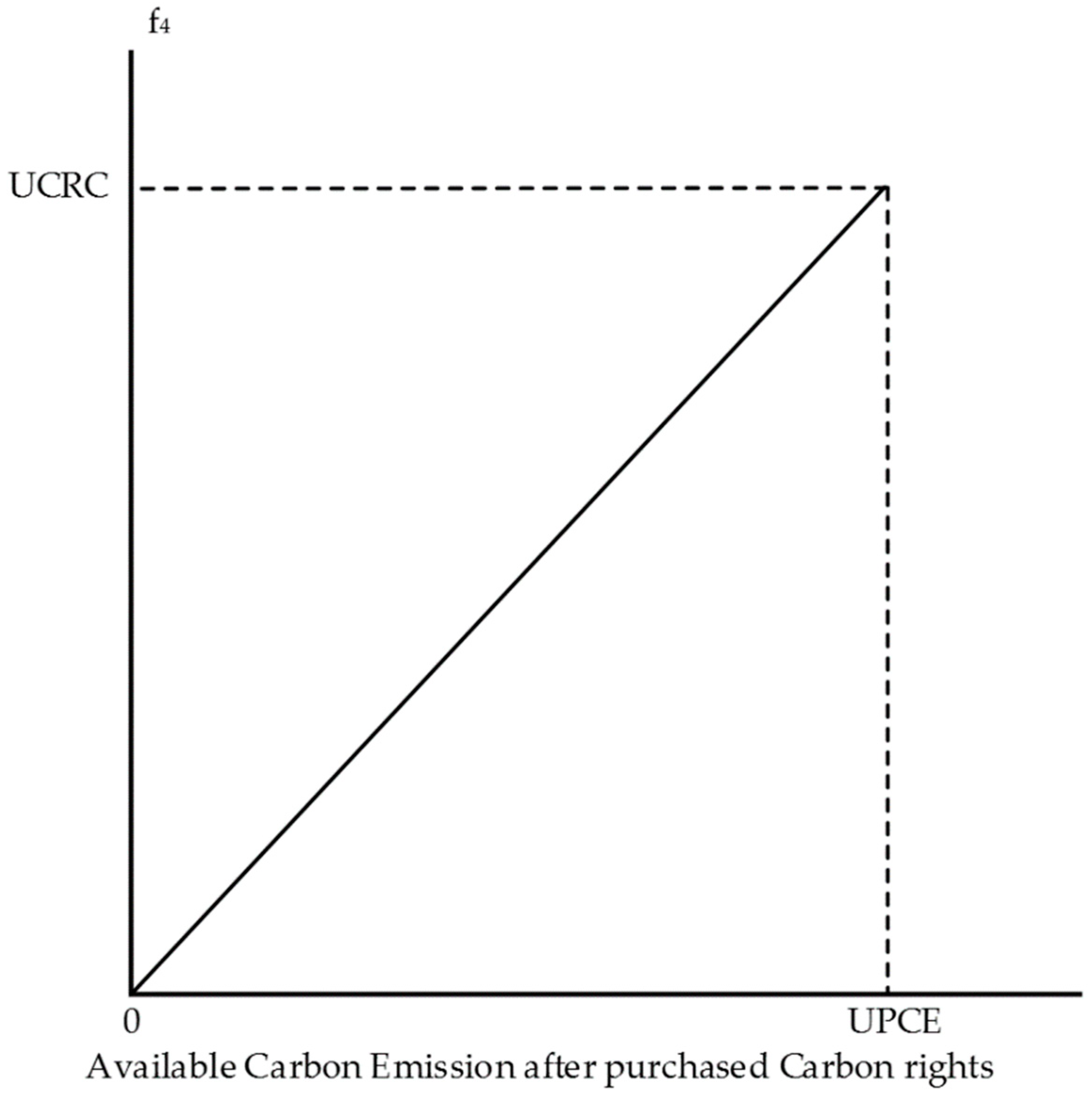
In recent years, there have been many studies to estimate the impact of CT on production through ABC [17,22,23]. However, there have been few articles that consider CRC in their decision model through ABC. In Model 2, we assume that the company can purchase CR at a single CRC rate (r) for any carbon emissions needed to receive the opportunity of additional sales. The CRC function can be represented as shown in Equation (18) and Figure 5. In Equation (18), ${\mathrm{f}}_4\left(\mathrm{g}-\mathrm{LCE}\right)$ is a CRC function, which is a function of CR purchase quantity $\left(\mathrm{g}-\mathrm{LCE}\right)$. Assume that the upper limit of the carbon emissions purchase quantity is UPCE. The upper limit on the carbon emissions the company can emit is $\mathrm{LPCE} = \mathrm{LCE} + \mathrm{UPCE}$ and its CRC at UPCE is UCRC. Thus, the carbon emissions cost function in Model 2 can be represented as shown in Equation (17):

$${\mathrm{f}}_3\left(\mathrm{g}\right)=\{\begin{array}{cc}\hfill {\mathrm{f}}_2\left(\mathrm{g}\right), & \mathrm{If} 0\le \mathrm{g}\le \mathrm{LCE} \hfill \\ \hfill {\mathrm{f}}_2\left(\mathrm{g}\right)+{\mathrm{f}}_4\left(\mathrm{g}-\mathrm{LCE}\right), & \mathrm{If} \mathrm{LCE}<\mathrm{g}\le \mathrm{LPCE} \left(=\mathrm{LCE}+\mathrm{YPCE}\right)\hfill \end{array}$$

(17)

$${\mathrm{f}}_4\left(\mathrm{g}-\mathrm{LCE}\right)=\mathrm{r}\ast \left(\mathrm{g}-\mathrm{LCE}\right).$$

(18)

Equation (17) can be formulated as Equations (19)–(23) in the mathematical programming model. Equation (19) is the carbon emissions cost function of Model 2, and Equaitons (20)–(23) and Equations (4)–(15) are the constraints associated with the carbon emissions cost function of Model 2.

Carbon emissions cost of Model 2:

$$\begin{array}{ll}\mathrm{CEC}& =\left({\mathrm{CTC}}_1{\mathsf{\mu }}_1+{\mathrm{CTC}}_2{\mathsf{\mu }}_2+{\mathrm{CTC}}_3{\mathsf{\mu }}_3\right){\mathsf{\delta }}_1\\ & + \left[\left({\mathrm{CTC}}_1{\mathsf{\mu }}_1+{\mathrm{CTC}}_2{\mathsf{\mu }}_2+{\mathrm{CTC}}_3{\mathsf{\mu }}_3\right)+\left(\mathrm{g}-\mathrm{LCE}\right)\ast \mathrm{r}\right]{\mathsf{\delta }}_2\end{array}$$

(19)

The associated constraints are:

$$\mathrm{g}={\displaystyle \sum _{\mathrm{i}=1}^{\mathrm{n}}}{\displaystyle \sum _{\mathrm{j} = 1,2,5}^{}}{\mathrm{CE}}_{\mathrm{im}}{\mathrm{X}}_{\mathrm{i}}={\mathsf{\varphi }}_1+{\mathsf{\varphi }}_2$$

(20)

$$0\le {\mathsf{\varphi }}_1\le {\mathsf{\delta }}_1\mathrm{LCE}$$

(21)

$${\mathsf{\delta }}_2\mathrm{LCE}<{\mathsf{\varphi }}_2\le {\mathsf{\delta }}_2\mathrm{LPCE}$$

(22)

$${\mathsf{\delta }}_1+{\mathsf{\delta }}_2=1,$$

(23)

where:

CEC	The carbon emissions cost including the carbon tax and carbon rights.
LPCE	The upper limit of the carbon emissions quantity the company can emit.
UPCE	The upper limit of the carbon emissions purchase quantity.
r	The single carbon rights cost rate.
${\mathsf{\varphi }}_1$	The company’s total CE quantity when g$\le \mathrm{LCE}.$
${\mathsf{\varphi }}_2$	The company’s total CE quantity when g $>\mathrm{LCE}.$
${\mathsf{\delta }}_1,{ \mathsf{\delta }}_2$	A special ordered set of type 1 (SOS1) of 0–1 variables in which only one variable can be 1; ${\mathsf{\delta }}_1=1$ means that the company does not need to purchase carbon rights, and ${ \mathsf{\delta }}_2=1$ means that the company needs to purchase carbon rights.

$({\mathsf{\delta }}_1, {\mathsf{\delta }}_2)$ is a special ordered set of type 1 (SOS1) of 0–1 variables in which only one variable can be 1. If ${\mathsf{\delta }}_1=1$, then ${\mathsf{\delta }}_2=0$ from Equation (23), and $0\le \mathrm{g}={\mathsf{\varphi }}_1\le \mathrm{LCE}$ from Equations (20) and (21). This means that the company does not need to purchase CR. The total carbon emissions cost is $\left({\mathrm{CTC}}_1{\mathsf{\mu }}_1+{\mathrm{CTC}}_2{\mathsf{\mu }}_2+{\mathrm{CTC}}_3{\mathsf{\mu }}_3\right)$ from Equation (19), including only the carbon tax cost. If ${\mathsf{\delta }}_2=1$, then ${\mathsf{\delta }}_1=0$ from Equation (23), and $\mathrm{LCE}<\mathrm{g}={\mathsf{\varphi }}_2\le \mathrm{LPCE}$ from Equations (20) and (22). This means that the company needs to purchase CR. The total carbon emissions cost is $\left[\left({\mathrm{CTC}}_1{\mathsf{\mu }}_1+{\mathrm{CTC}}_2{\mathsf{\mu }}_2+{\mathrm{CTC}}_3{\mathsf{\mu }}_3\right)+\mathrm{r}\ast \left(\mathrm{g}-\mathrm{LCE}\right)\right]$ from Equation (19), including the carbon tax cost and the CRC. The associated constraints associated with the carbon tax cost are shown as Equations (4)–(15).

3.1.5. Carbon Emissions Cost with Carbon Trading of MOQCE—Model 3

In Model 3, it is assumed that the company can purchase CR through carbon trading of a minimum order quantity of carbon emissions (MOQCE) based on the Carbon Financial Instrument from the Chicago Climate Exchange (CCX) to allow additional sales. The company should purchase the minimum quantity of CE rights with a fixed carbon rights cost (FCRC). The carbon rights cost function of Model 3 can be represented as in Figure 6, and its related carbon emissions cost can be represented as in Equation (24). In Equation (24), ${\mathrm{f}}_2\left(\mathrm{g}\right)$ is the carbon tax function and ${\mathrm{f}}_3\left(\mathrm{g}\right)$ is the carbon emissions cost function, where ${\mathrm{f}}_2\left(\mathrm{g}\right)$ and ${\mathrm{f}}_3\left(\mathrm{g}\right)$ are the function of the company’s total CE quantity (g). LCE is the carbon emissions quantity that the company can emit, as limited or allocated by the government; MBCE is the maximum buyable CE quantity that the company can purchase in the market; LMCE is the company’s maximum total CE quantity that the company can emit when the company purchases at MOQCE; LMPCE is the company’s total CE quantity when the company purchases CR at the MBCE; and sr is the single carbon rights cost rate when the company purchases a CE quantity that is greater than MOQCE. That is, the carbon emissions cost includes only the carbon tax cost when $0\le \mathrm{g}\le \mathrm{LCE}$. The carbon emissions cost includes the carbon tax cost ${\mathrm{f}}_2\left(\mathrm{g}\right)$ and the fixed carbon rights cost at MOQCE (i.e., FCRC) when $\mathrm{LCE}\le \mathrm{g}\le \mathrm{LMCE}$, and the carbon emissions cost includes the carbon tax cost ${\mathrm{f}}_2\left(\mathrm{g}\right)$, the fixed carbon rights cost at MOQCE (i.e., FCRC), and CRC over MOQCE [i.e., $\mathrm{sr}\ast \left(\mathrm{g}-\mathrm{MOQCE}-\mathrm{LCE}\right)$] when $\mathrm{LMCE}<\mathrm{g}\le \mathrm{LMPCE}$.

$${\mathrm{f}}_3\left(\mathrm{g}\right)=\{\begin{array}{cc}\hfill {\mathrm{f}}_2\left(\mathrm{g}\right), & \mathrm{If} 0\le \mathrm{g}\le \mathrm{LCE}\hfill \\ \hfill {\mathrm{f}}_2\left(\mathrm{g}\right)+\mathrm{FCRC}, & \mathrm{If} \mathrm{LCE}\le \mathrm{g}\le \mathrm{LMCE} \left(=\mathrm{LCE}+\mathrm{MOQCE}\right) \hfill \\ \hfill {\mathrm{f}}_2\left(\mathrm{g}\right)+\mathrm{FCRC}+\mathrm{sr}\ast \left(\mathrm{g}-\mathrm{MOQCE}-\mathrm{LCE}\right), & \mathrm{If} \mathrm{LMCE}<\mathrm{g}\le \mathrm{LMPCE}\left(=\mathrm{LCE}+\mathrm{MBCE}\right)\hfill \end{array}$$

(24)

Equation (24) can be formulated as Equations (25)–(31) in the mathematical programming model. Equation (24) is the carbon emissions cost function of Model 3, and Equations (25)–(31) and (4)–(15) are the constraints associated with the carbon emissions cost function of Model 3.

Carbon emissions cost of Model 3:

$$\begin{array}{ll}\mathrm{CEC}& ={\mathsf{\delta }}_1\left({\mathrm{CTC}}_1{\mathsf{\mu }}_1+{\mathrm{CTC}}_2{\mathsf{\mu }}_2+{\mathrm{CTC}}_3{\mathsf{\mu }}_3\right)\\ & +{\mathsf{\delta }}_{20}\left[\left({\mathrm{CTC}}_1{\mathsf{\mu }}_1+{\mathrm{CTC}}_2{\mathsf{\mu }}_2+{\mathrm{CTC}}_3{\mathsf{\mu }}_3\right)+\mathrm{FCRC}\right]\\ & +{\mathsf{\delta }}_{21}\left[\left({\mathrm{CTC}}_1{\mathsf{\mu }}_1+{\mathrm{CTC}}_2{\mathsf{\mu }}_2+{\mathrm{CTC}}_3{\mathsf{\mu }}_3\right)+\mathrm{FCRC}+\mathrm{sr}\ast \left(\mathrm{g}-\mathrm{MOQCE}-\mathrm{LCE}\right)\right]\end{array}$$

(25)

The associated constraints are:

$$\mathrm{g}={\displaystyle \sum _{\mathrm{i}=1}^{\mathrm{n}}}{\displaystyle \sum _{\mathrm{m}=1}^3}{\mathrm{CE}}_{\mathrm{im}}{\mathrm{X}}_{\mathrm{i}}={\mathsf{\varphi }}_1+{\mathsf{\varphi }}_{20}+{\mathsf{\varphi }}_{21}$$

(26)

$$0\le {\mathsf{\varphi }}_1\le {\mathsf{\delta }}_1\mathrm{LCE}$$

(27)

$${\mathsf{\delta }}_{20}\mathrm{LCE}<{\mathsf{\varphi }}_{20}\le {\mathsf{\delta }}_{20}\mathrm{LMCE}$$

(28)

$${\mathsf{\delta }}_{21}\mathrm{LMCE}<{\mathsf{\varphi }}_{21}\le {\mathsf{\delta }}_{21}\mathrm{LMPCE}$$

(29)

$${\mathsf{\delta }}_1+{\mathsf{\delta }}_{20}+{\mathsf{\delta }}_{21}=1$$

(30)

$${\mathsf{\delta }}_1,{\mathsf{\delta }}_{20},{ \mathsf{\delta }}_{21}=0,1,$$

(31)

where:

MOQCE	The minimum order quantity of carbon emissions.
FCRC	The fixed carbon rights cost at MOQCE.
LMCE	The company’s maximum total CE quantity that the company can emit when the company purchases at MOQCE; $\mathrm{LMCE}=\mathrm{LCE}+\mathrm{MOQCE}$.
MBCE	The maximum buyable CE quantity that the company can purchase in the market.
LMPCE	The company’s total CE quantity when the company purchases carbon rights at the MBCE; $\mathrm{LMPCE}\left(=\mathrm{LCE}+\mathrm{MBCE}\right)$.
sr	The single carbon rights cost rate when the company purchases a CE quantity that is greater than MOQCE.
${\mathsf{\varphi }}_1$	The company’s total CE quantity when g$={\mathsf{\varphi }}_1\le \mathrm{LCE}.$
${\mathsf{\varphi }}_{20}$	The company’s total CE quantity when $\mathrm{LCE}\le \mathrm{g}={\mathsf{\varphi }}_{20}\le \mathrm{LMCE}.$
${\mathsf{\varphi }}_{21}$	The company’s total CE quantity when $\mathrm{LMCE}<\mathrm{g}={\mathsf{\varphi }}_{21}\le \mathrm{LMPCE}$.
${\mathsf{\delta }}_1,{ \mathsf{\delta }}_{20},{\mathsf{\delta }}_{21}$	A special ordered set of type 1 (SOS1) of 0–1 variables in which only one variable can be 1; ${\mathsf{\delta }}_1=1$ means that the company does not need to purchase carbon rights; ${\mathsf{\delta }}_{20}=1$ means that the company needs to purchase carbon rights at MOQCE; and ${\mathsf{\delta }}_{21}=1$ means that the company needs to purchase carbon rights over MOQCE.

$({\mathsf{\delta }}_1,{ \mathsf{\delta }}_2,{ \mathsf{\delta }}_3)$ is a special ordered set of type 1 (SOS1) of 0–1 variables in which only one variable can be 1. If ${\mathsf{\delta }}_1=1$, then ${\mathsf{\delta }}_{20},{ \mathsf{\delta }}_{21}=0$, from Equation (30), and $0\le \mathrm{g}={\mathsf{\varphi }}_1\le \mathrm{LCE}$ from Equations (26) and (27). This means that the company does not need to purchase CR. The total carbon emissions cost is $\left({\mathrm{CTC}}_1{\mathsf{\mu }}_1+{\mathrm{CTC}}_2{\mathsf{\mu }}_2+{\mathrm{CTC}}_3{\mathsf{\mu }}_3\right)$ from Equation (25), including only the carbon tax cost. If ${\mathsf{\delta }}_{20}=1$, then ${\mathsf{\delta }}_1={\mathsf{\delta }}_{21}=0$ from Equation (30), and $\mathrm{LCE}<\mathrm{g}={\mathsf{\varphi }}_{20}\le \mathrm{LMCE}$ from Equations (26) and (28). This means that the company needs to purchase CR at MOQEC. The total carbon emissions cost is $\left[\left({\mathrm{CTC}}_1{\mathsf{\mu }}_1+{\mathrm{CTC}}_2{\mathsf{\mu }}_2+{\mathrm{CTC}}_3{\mathsf{\mu }}_3\right)+\mathrm{FCRC}\right]$ from Equation (25), including the carbon tax cost and the fixed carbon rights costs at MOQCE (i.e., FCRC). If ${\mathsf{\delta }}_{21}=1$, then ${\mathsf{\delta }}_1={\mathsf{\delta }}_{20}=0$ from Equation (30), and $\mathrm{LMCE}<\mathrm{g}={\mathsf{\varphi }}_{21}\le \mathrm{LMPCE}$ from Equations (26) and (29). This means that the company needs to purchase CR over MOQEC. The total carbon emissions cost is $\left[\left({\mathrm{CTC}}_1{\mathsf{\mu }}_1+{\mathrm{CTC}}_2{\mathsf{\mu }}_2+{\mathrm{CTC}}_3{\mathsf{\mu }}_3\right)+\mathrm{FCRC}+\left(\mathrm{g}-\mathrm{MOQCE}-\mathrm{LCE}\right)\ast \mathrm{sr}\right]$ from Equation (25), including the carbon tax cost, the fixed carbon rights cost at MOQCE (i.e., FCRC), and the carbon rights cost over MOQCE (i.e., $\mathrm{sr}\ast \left(\mathrm{g}-\mathrm{MOQCE}-\mathrm{LCE}\right)$). The associated constraints associated with the carbon tax cost are given in Equations (4)–(15).

3.2. Unit Level—The Consumption of Direct Labor Cost Function

The direct labor of knitted production includes regular hours and overtime, which can be used in the activities of bottom trimming and assembling at the unit level activity. The cost of regular hours is fixed for the company in the short term, as the company needs to pay for these workers whether or not they are part of the workforce. However, the labor capacity could increase through overtime in the short term owing to rush orders or orders that cannot be completed on time.

In the production of knitted footwear, numerous manual processes have been changed and combined into a simple knitting activity, thereby reducing the number of direct labor hours (DLH) and the direct labor costs (DLC). Therefore, assume that the processes that require workers include bottom trimming (j = 4) and assembling (j = 5). The total direct labor cost (TDLC) function is a continuous piecewise linear function, as shown in Figure 7. If the direct labor hours needed exceed the regular working hours, there will be two sets of labor hours paid at two different wage rates.

The direct labor cost function in Figure 7 can be formulated as in Equations (31)–(41) in the mathematical programming model. Equation (31) is the direct labor cost function that will be included in the objective function, and Equations (32)–(41) are the associated constraints. Assume that the wage rates in the three ranges of direct labor hours shown in Figure 7 are WR₀, WR₁, and WR₂.

Direct labor costs:

$$\mathrm{TDLC}={\mathrm{DLC}}_0+{\mathsf{\gamma }}_1\left({\mathrm{ODLC}}_1-{\mathrm{DLC}}_0\right)+{\mathsf{\gamma }}_2\left({\mathrm{ODLC}}_2-{\mathrm{DLC}}_0\right).$$

(31)

The associated constraints are:

$$\mathrm{TDLH}={\displaystyle \sum _{\mathrm{i}=1}^{\mathrm{n}}}\left({\mathrm{LH}}_{\mathrm{i}4}+{\mathrm{LH}}_{\mathrm{i}5}\right){\mathrm{X}}_{\mathrm{i}}\le {\mathsf{\gamma }}_0{\mathrm{DLH}}_0+{\mathsf{\gamma }}_1\left({\mathrm{ODLH}}_1-{\mathrm{DLH}}_0\right)+{\mathsf{\gamma }}_2\left({\mathrm{ODLH}}_2-{\mathrm{DLH}}_0\right)$$

(32)

$${\mathsf{\gamma }}_0-{\mathsf{\Gamma }}_1\le 0$$

(33)

$${\mathsf{\gamma }}_1-{\mathsf{\Gamma }}_1-{\mathsf{\Gamma }}_2\le 0$$

(34)

$${\mathsf{\gamma }}_2-{\mathsf{\Gamma }}_2\le 0$$

(35)

$${\mathsf{\gamma }}_0+{\mathsf{\gamma }}_1+{\mathsf{\gamma }}_2=1$$

(36)

$${\mathsf{\Gamma }}_1+{\mathsf{\Gamma }}_2=1$$

(37)

$${\mathsf{\Gamma }}_1,{\mathsf{\Gamma }}_2=0, 1$$

(38)

$$0\le {\mathsf{\gamma }}_0\le 1$$

(39)

$$0\le {\mathsf{\gamma }}_1\le 1$$

(40)

$$0\le {\mathsf{\gamma }}_2\le 1$$

(41)

variables:

${\mathrm{X}}_1$	The quantity of product i.
${\mathsf{\gamma }}_0,{ \mathsf{\gamma }}_1,{\mathsf{\gamma }}_2$	A set of non-negative variables of SOS2 (special ordered set of type 2).
${\mathsf{\Gamma }}_1,{\mathsf{\Gamma }}_2$	A set of 0-1 indicator variables of SOS1 (special ordered set of type 1).
parameters:
${\mathrm{LH}}_{\mathrm{i}4}$	The labor hours required for one unit of product i during the bottom trimming (j = 4).
${\mathrm{LH}}_{\mathrm{i}5}$	The labor hours required for one unit of product i during the assembling (j = 5).
${\mathrm{DLH}}_0$	The total regular direct labor hours, as shown in Figure 7.
${\mathrm{ODLH}}_1$	The highest overtime hours with the first overtime pay rate, as shown in Figure 7.
${\mathrm{ODLH}}_2$	The highest overtime hours with the second overtime pay rate, as shown in Figure 7.
${\mathrm{DLC}}_0$	The total regular direct labor costs at ${\mathrm{DLH}}_0$, i.e., DLC0 = WR0 * DLH0.
${\mathrm{ODLC}}_1$	The total regular direct labor costs at ${\mathrm{ODLH}}_1$, i.e., ODLC1 = DLC0 + WR1 * (ODLH1 − DLH0).
${\mathrm{ODLC}}_2$	The total regular direct labor costs at ${\mathrm{ODLH}}_2$, i.e., ODLC2 = ODLC1 + WR2 * (ODLH2 − ODLH1).

(γ₀, γ₁, γ₂) is a special ordered set of type 2 (SOS2) non-negative variables, and (${\mathsf{\Gamma }}_1,{\mathsf{\Gamma }}_2)$ is a special ordered set of type 1 (SOS1) 0–1 variables. If ${\mathsf{\Gamma }}_1=1,$ then ${\mathsf{\Gamma }}_2=0$from Equation (37), and $0\le {\mathsf{\gamma }}_0,{ \mathsf{\gamma }}_1\le 1$ and ${\mathsf{\gamma }}_0+{\mathsf{\gamma }}_1=1$ from Equations (33), (34) and (36). Thus, the company’s total direct labor hour is [${\mathsf{\gamma }}_0{\mathrm{DLH}}_0+{\mathsf{\gamma }}_1\left({\mathrm{ODLH}}_1-{\mathrm{DLH}}_0\right)]$ from Equation (32) and the total direct labor cost is $[{\mathrm{DLC}}_0+{\mathsf{\gamma }}_1\left({\mathrm{ODLC}}_1-{\mathrm{DLC}}_0\right)]$ from Equation (31). This means that the company’s direct labor hours fall within the second range of Figure 7, and ($\mathrm{TDLH}$, $\mathrm{TDLC}$) is the linear combination of $\left({\mathrm{DLH}}_0,{ \mathrm{DLC}}_0\right)$ and $\left({\mathrm{ODLH}}_1,{ \mathrm{ODLC}}_1\right)$.

If ${\mathsf{\Gamma }}_2=1$, then ${\mathsf{\Gamma }}_1=0$ from Equation (37), and $0\le {\mathsf{\gamma }}_1,{ \mathsf{\gamma }}_2\le 1$ and ${\mathsf{\gamma }}_1+{\mathsf{\gamma }}_2=1$ from Equations (34)–(36). Thus, the company’s total direct labor hours is [${\mathsf{\gamma }}_1\left({\mathrm{ODLH}}_1-{\mathrm{DLH}}_0\right)+{\mathsf{\gamma }}_2\left({\mathrm{ODLH}}_2-{\mathrm{DLH}}_0\right)]$ from Equation (32), and the total direct labor cost is $\left[{\mathsf{\gamma }}_1\left({\mathrm{ODLC}}_1-{\mathrm{DLC}}_0\right)+{\mathsf{\gamma }}_2\left({\mathrm{ODLC}}_2-{\mathrm{DLC}}_0\right)\right]$ from Equation (31). This means that the company’s direct labor hours fall within the third range of Figure 7, and ($\mathrm{TDLH}$,$\mathrm{TDLC}$) is the linear combination of $\left({\mathrm{ODLH}}_1,{ \mathrm{ODLC}}_1\right)$ and $\left({\mathrm{ODLH}}_2,{ \mathrm{ODLC}}_2\right)$.

If ${\mathsf{\gamma }}_0=1{ \mathrm{and} \mathsf{\Gamma }}_1=1,{ \mathrm{then} \mathsf{\gamma }}_1={\mathsf{\gamma }}_2=0$ from Equation (36), ${\mathsf{\Gamma }}_2=0$ from Equation (37), $\mathrm{TDLH}={\displaystyle {\sum }_{\mathrm{i}=1}^{\mathrm{n}}}\left({\mathrm{LH}}_{\mathrm{i}4}+{\mathrm{LH}}_{\mathrm{i}5}\right){\mathrm{X}}_{\mathrm{i}}\leqq {\mathsf{\gamma }}_0{ \mathrm{DLH}}_0$ from Equation (32), and $\mathrm{TDLC}={\mathrm{DLC}}_0$ from Equation (31). This means that the company’s direct labor hours fall within the first range of Figure 7 and the total direct labor cost is ${\mathrm{DLC}}_0$.

3.3. Capacity of Machine Hours

Assume that the manufacturing process of knitted products in this study has three kinds of automatic machines that can replace manual activities to improve efficiency. The knitting machine is used to knit the vamp (j = 1), the pressing machine is used to generate the shoe’s bottom (j = 2), and the automatic gluing machine is used to assemble the vamps and bottoms to the footwear during assembling (j = 5). Moreover, the three kinds of machines have upper limits for useable machine hours, facility regions, and worker usage. Assume that the other related costs are fixed at “φ”, including machine depreciation. The machine hour constraints are shown in Equations (42)–(44):

$${\displaystyle \sum _{\mathrm{i}=1}^{\mathrm{n}}}{\mathrm{MH}}_{\mathrm{i}1}{\mathrm{X}}_{\mathrm{i}}\le { \mathrm{LMH}}_1$$

(42)

$${\displaystyle \sum _{\mathrm{i}=1}^{\mathrm{n}}}{\mathrm{MH}}_{\mathrm{i}2}{\mathrm{X}}_{\mathrm{i}}\le { \mathrm{LMH}}_2$$

(43)

$${\displaystyle \sum _{\mathrm{i}=1}^{\mathrm{n}}}{\mathrm{MH}}_{\mathrm{i}5}{\mathrm{X}}_{\mathrm{i}}\le { \mathrm{LMH}}_5,$$

(44)

where

Xi	The quantity of product i.
${\mathrm{MH}}_{\mathrm{i}1}$	The machine hours of the knitting machine required for one unit of product i.
${\mathrm{MH}}_{\mathrm{i}2}$	The machine hours of the pressing machine required for one unit of product i.
${\mathrm{MH}}_{\mathrm{i}5}$	The machine hours of the gluing machine required for one unit of product i.
${\mathrm{LMH}}_1$	The capability of machine hours for the knitting machine.
${\mathrm{LMH}}_2$	The capability of machine hours for the pressing machine.
${\mathrm{LMH}}_5$	The capability of machine hours for the gluing machine.

3.4. Batch-Level Activity Cost Function for Setup and Material Handling Activities

The model in this paper assumed there are three kinds of activities that can be classified as batch-level activities in the process of knitted shoes: molding the bottom (j = 3), setting up (j = 6) to produce different kinds of vamps or bottoms, and material handling (j = 7). Let the set B = {3, 6, 7} for the batch-level activities. The overall batch-level activity costs can be represented as (${{\displaystyle \sum }}_{\mathrm{i}=1}^{\mathrm{n}}{{\displaystyle \sum }}_{\mathrm{j}\in \mathsf{\beta }}{\mathsf{\Theta }}_{\mathrm{j}}{\mathsf{\Lambda }}_{\mathrm{ij}}{\mathsf{\beta }}_{\mathrm{ij}})$, which is included in the objective function of total profit. The associated constraints are as shown in Equations (45) and (46):

$${\mathrm{X}}_{\mathrm{i}}\le {\mathsf{\Theta }}_{\mathrm{ij}}{\mathsf{\beta }}_{\mathrm{ij}} \mathrm{i}=1,2,3; \mathrm{j} \in \mathrm{B}$$

(45)

$${\displaystyle \sum _{\mathrm{i}=1}^{\mathrm{n}}}{\mathsf{\Lambda }}_{\mathrm{ij}}{\mathsf{\beta }}_{\mathrm{ij}}\le {\mathrm{T}}_{\mathrm{j}}{ \mathsf{\beta }}_{\mathrm{ij}}\ge 0; \mathrm{j} \in \mathrm{B}$$

(46)

where:

${\mathrm{X}}_{\mathrm{i}}$	The quantity of product i.
${\mathsf{\beta }}_{\mathrm{ij}}$	The number of batches of batch-level activity j (j ∈ B) for product i.
${\mathsf{\Theta }}_{\mathrm{ij}}$	The quantity of product i for each batch of batch-level activity j (j ∈ B).
${\mathsf{\Lambda }}_{\mathrm{ij}}$	The resource consumption of each batch of batch-level activity j (j ∈ B) for product i.
${\mathrm{T}}_{\mathrm{j}}$	The capacity of the activity driver of batch-level activity j (j ∈ B).

Equation (45) is the constraint concerning the product’s quantity, which cannot be greater than the total quantity of all batches. Equation (46) is the constraint concerning the resource limitations (${\mathrm{T}}_{\mathrm{j}}$) for batch-level activity j.

3.5. Product-Level Activity Cost Function—Product Design

The company needs to produce different kinds of products in order to meet the various demands in the market. There are three styles of knitted footwear produced by the company, including Mary Janes (Product 1), dress athletic-inspired footwear (Product 2), and high-top footwear (Product 3), and the cost of product design was included in this study as a production-level activity. The overall product-level activity cost can be represented as (${{\displaystyle \sum }}_{\mathrm{i}=1}^{\mathrm{n}}{{\displaystyle \sum }}_{\mathrm{j}\in \mathrm{P}}{\mathrm{MD}}_{\mathrm{i}}{\mathsf{\Pi }}_{\mathrm{ij}}{\mathrm{P}}_{\mathrm{i}})$, which is included in the objective function of the total profit. The associated constraints are shown in Equations (47) and (48):

$${\mathrm{X}}_{\mathrm{i}}\le {\mathrm{MD}}_{\mathrm{i}}{\mathsf{\alpha }}_{\mathrm{i}} \mathrm{i}=1,2,3;$$

(47)

$${\displaystyle \sum _{\mathrm{i}=1}^{\mathrm{n}}}{\mathsf{\Pi }}_{\mathrm{ij}}{\mathsf{\alpha }}_{\mathrm{i}}\le {\mathrm{C}}_{\mathrm{j}} \mathrm{j}\in \mathrm{P}$$

(48)

where:

${\mathrm{X}}_{\mathrm{i}}$	The quantity of product i.
${\mathrm{MD}}_{\mathrm{i}}$	The market demand of product i.
${\mathsf{\alpha }}_{\mathrm{i}}$	An indicator variable for whether product i is produced and sold; ${\mathsf{\alpha }}_{\mathrm{i}}=1$ means that product i will be produced and sold, otherwise, ${\mathsf{\alpha }}_{\mathrm{i}}=0$.
${\mathsf{\Pi }}_{\mathrm{ij}}$	The requirement of the activity driver of product-level activity j (j ∈ P) for product i.
${\mathrm{C}}_{\mathrm{j}}$	The capacity of the activity drivers for product-level activity j (j ∈ P).

Equation (47) is the constraint concerning the product’s quantity, which cannot be greater than the market demand of product i. Equation (48) is the constraint concerning the resource limitations (${\mathrm{C}}_{\mathrm{j}}$) for batch-level activity j.

3.6. Direct Material Costs

The manufacturers of knitted shoes in this study use thread, polyurethane (PU), and glue as the main direct materials in the three activities to produce knitted footwear: knitting (j = 1), pressing (j = 2), and assembling (j = 5). The total material cost is [${{\displaystyle \sum }}_{\mathrm{i}=1}^{\mathrm{n}}\left({{\displaystyle \sum }}_{\mathrm{k}=1}^3{\mathrm{CM}}_{\mathrm{k}}{\mathrm{MR}}_{\mathrm{ik}}\right){\mathrm{X}}_{\mathrm{i}}]$, which is included in the objective function of the total profit. The material constraint is shown in Equation (49):

$${\displaystyle \sum _{\mathrm{I}=1}^{\mathrm{n}}}{(\mathrm{MR}}_{\mathrm{ik}}{\mathrm{X}}_{\mathrm{i}})\le { \mathrm{MQ}}_{\mathrm{k}} \mathrm{k}=1, 2, 3$$

(49)

where:

${\mathrm{X}}_{\mathrm{i}}$	The quantity of product i.
${\mathrm{CM}}_{\mathrm{k}}$:	The unit cost of material k.
${\mathrm{MR}}_{\mathrm{ik}}$	The quantity of material k required for one unit of product i.
${\mathrm{MQ}}_{\mathrm{k}}$	The quantity of material k available for production.

3.7. Assumptions

The activity-based costing (ABC) approach is used by manufacturers to get more accurate, detailed cost assignments for activities by using activity drivers [21], which can help manufacturers effectively collect and control relevant cost data [75,76,77]. Without a loss of generality, the Green Production Decision Model with Carbon Emissions (GPDMCE) proposed in this paper could be used to explore the impact of CE in the knitted footwear industry.

In the models explored in this paper, there were some assumptions. First, the overhead activities in GPDMCE were divided into the unit level, batch level, and product level [21] by the ABC approach, and their resources and activity drivers were also investigated and selected using the ABC approach [16,78]. Second, the capacity of machine hours was fixed for manufacturers in the short term. Third, depreciation and machine costs were considered as fixed costs, and there were limited machine hours for manufacturers to produce products. Fourth, overtime hours would be paid at a higher rate than normal labor hours. Fifth, the environmental issues considered in this paper were the effect on CE of carbon taxes and cap & trade. Sixth, the CE permits would not be sold to other companies after purchase. Seventh, GPDMCE is used because it gives data about the direct materials, direct labor, machining of products and so on that a manufacturer can use to produce final goods. We assume that these data can be collected to effectively reflect the manufacturing situation and that these data can help researchers to simulate the production process.

3.8. Objective Function

This paper proposed three models of GPDMCE combining ABC with TOC to achieve the optimal product mix and profit in the knitted footwear industry. These models were also used to explore the effect of carbon emissions. The objective function was to maximize total profit (π):

$$\begin{array}{ll}\mathrm{Maximize} \mathsf{\pi } & = \mathrm{total} \mathrm{revenue} \mathrm{of} \mathrm{knitted} \mathrm{footwear} - \mathrm{total} \mathrm{direct} \mathrm{material} \mathrm{costs}\\ & \hspace{1em}\hspace{1em}\hspace{1em}- \mathrm{total} \mathrm{direct} \mathrm{labor} \mathrm{costs}-\mathrm{total} \mathrm{batch} \mathrm{level} \mathrm{activity} \mathrm{costs}\\ & \hspace{1em}\hspace{1em}\hspace{1em}-\mathrm{total} \mathrm{product} \mathrm{level} \mathrm{activity} \mathrm{cost}-\mathrm{total} \mathrm{carbon} \mathrm{emissions} \mathrm{cost}\\ & \hspace{1em}\hspace{1em}\hspace{1em}-\mathrm{total} \mathrm{fixed} \mathrm{costs} \left(\mathrm{depreciation} \mathrm{and} \mathrm{other} \mathrm{fixed} \mathrm{cost}\right)\end{array}$$

3.8.1. Model 1: Carbon Emissions Costs without Carbon Trading

Model 1 considers only the carbon tax as the carbon emissions cost imposed by the government. The objective is to maximize the total profit, as shown in Equation (50). The associated constraints include Equations (4)–(16) and (32)–(49):

$$\begin{array}{ll}\mathrm{Maximize} \mathsf{\pi }& ={\displaystyle \sum _{\mathrm{i}=1}^{\mathrm{n}}}{\mathrm{SP}}_{\mathrm{i}}{\mathrm{X}}_{\mathrm{i}}-{\displaystyle \sum _{\mathrm{i}=1}^{\mathrm{n}}}\left({\displaystyle \sum _{\mathrm{k}=1}^3}{\mathrm{CM}}_{\mathrm{k}}{\mathrm{MR}}_{\mathrm{ik}}\right){\mathrm{X}}_{\mathrm{i}}-[{\mathrm{DLC}}_0+{\mathsf{\gamma }}_1\left({\mathrm{ODLC}}_1-{\mathrm{DLC}}_0\right)\\ & \hspace{1em}\hspace{1em}+{\mathsf{\gamma }}_2\left({\mathrm{ODLC}}_2-{\mathrm{DLC}}_0\right)]-{\displaystyle \sum _{\mathrm{i}=1}^{\mathrm{n}}}{\displaystyle \sum _{\mathrm{j}\in \mathsf{\beta }}}{\Theta }_{\mathrm{j}}{\mathsf{\Lambda }}_{\mathrm{ij}}{\mathsf{\beta }}_{\mathrm{ij}}-{\displaystyle \sum _{\mathrm{i}=1}^{\mathrm{n}}}{\displaystyle \sum _{\mathrm{j}\in \mathrm{P}}}{\mathrm{MD}}_{\mathrm{i}}{\mathsf{\Pi }}_{\mathrm{ij}}{\mathrm{P}}_{\mathrm{i}}-({\mathrm{CTC}}_1{\mathsf{\mu }}_1\\ & \hspace{1em}\hspace{1em}+{\mathrm{CTC}}_2{\mathsf{\mu }}_2+{\mathrm{CTC}}_3{\mathsf{\mu }}_3)-\mathrm{F}\end{array}$$

(50)

3.8.2. Model 2: Carbon Emissions Cost with Carbon Trading of a Single Carbon Rights Cost Rate

Model 2 considers the carbon emissions cost with carbon trading of a single CRC rate. The objective is to maximize the total profit, as shown in Equation (51). The associated constraints include Equations (4)–(15), (20)–(23) and (32)–(49):

$$\begin{array}{ll}\mathrm{Maximize} \mathsf{\pi }& ={\displaystyle \sum _{\mathrm{i}=1}^{\mathrm{n}}}{\mathrm{SP}}_{\mathrm{i}}{\mathrm{X}}_{\mathrm{i}}-{\displaystyle \sum _{\mathrm{i}=1}^{\mathrm{n}}}\left({\displaystyle \sum _{\mathrm{k}=1}^3}{\mathrm{CM}}_{\mathrm{k}}{\mathrm{MR}}_{\mathrm{ik}}\right){\mathrm{X}}_{\mathrm{i}}\\ & \hspace{1em}\hspace{1em}\hspace{1em}-\left[{\mathrm{DLC}}_0+{\mathsf{\gamma }}_1\left({\mathrm{ODLC}}_1-{\mathrm{DLC}}_0\right)+{\mathsf{\gamma }}_2\left({\mathrm{ODLC}}_2-{\mathrm{DLC}}_0\right)\right]\\ & \hspace{1em}\hspace{1em}\hspace{1em}-{\displaystyle \sum _{\mathrm{i}=1}^{\mathrm{n}}}{\displaystyle \sum _{\mathrm{j}\in \mathsf{\beta }}}{\mathsf{\Theta }}_{\mathrm{j}}{\mathsf{\Lambda }}_{\mathrm{ij}}{\mathsf{\beta }}_{\mathrm{ij}}-{\displaystyle \sum _{\mathrm{i}=1}^{\mathrm{n}}}{\displaystyle \sum _{\mathrm{j}\in \mathrm{P}}}{\mathrm{MD}}_{\mathrm{i}}{\mathsf{\Pi }}_{\mathrm{ij}}{\mathrm{P}}_{\mathrm{i}}\\ & \hspace{1em}\hspace{1em}\hspace{1em}-[\left({\mathrm{CTC}}_1{\mathsf{\mu }}_1+{\mathrm{CTC}}_2{\mathsf{\mu }}_2+{\mathrm{CTC}}_3{\mathsf{\mu }}_3\right){\mathsf{\delta }}_1+(\left({\mathrm{CTC}}_1{\mathsf{\mu }}_1+{\mathrm{CTC}}_2{\mathsf{\mu }}_2+{\mathrm{CTC}}_3{\mathsf{\mu }}_3\right)\\ & \hspace{1em}\hspace{1em}\hspace{1em}+\left(\mathrm{g}-\mathrm{LCE}\ast \mathrm{r}\right){\mathsf{\delta }}_2]-\mathrm{F}\end{array}$$

(51)

3.8.3. Model 3: Carbon Emissions Cost with Carbon Trading of MOQCE

Model 3 considers the carbon emissions cost with carbon trading of MOQCE. The objective is to maximize the total profit, as shown in Equation (52). The associated constraints include Equations (4)–(14) and (26)–(49):

$$\begin{array}{ll}\mathrm{Maximize} \mathsf{\pi }& ={\displaystyle \sum _{\mathrm{i}=1}^{\mathrm{n}}}{\mathrm{SP}}_{\mathrm{i}}{\mathrm{X}}_{\mathrm{i}}-{\displaystyle \sum _{\mathrm{i}=1}^{\mathrm{n}}}\left({\displaystyle \sum _{\mathrm{k}=1}^3}{\mathrm{CM}}_{\mathrm{k}}{\mathrm{MR}}_{\mathrm{ik}}\right){\mathrm{X}}_{\mathrm{i}}\\ & \hspace{1em}\hspace{1em}\hspace{1em}-\left[{\mathrm{DLC}}_0+{\mathsf{\gamma }}_1\left({\mathrm{ODLC}}_1-{\mathrm{DLC}}_0\right)+{\mathsf{\gamma }}_2\left({\mathrm{ODLC}}_2-{\mathrm{DLC}}_0\right)\right]-{\displaystyle \sum _{\mathrm{i}=1}^{\mathrm{n}}}{\displaystyle \sum _{\mathrm{j}\in \mathsf{\beta }}}{\mathsf{\Theta }}_{\mathrm{j}}{\mathsf{\Lambda }}_{\mathrm{ij}}{\mathsf{\beta }}_{\mathrm{ij}}\\ & \hspace{1em}\hspace{1em}\hspace{1em}-{\displaystyle \sum _{\mathrm{i}=1}^{\mathrm{n}}}{\displaystyle \sum _{\mathrm{j}\in \mathrm{P}}}{\mathrm{MD}}_{\mathrm{i}}{\mathsf{\Pi }}_{\mathrm{ij}}{\mathrm{P}}_{\mathrm{i}}-{\mathsf{\delta }}_1({\mathrm{CTC}}_1{\mathsf{\mu }}_1+{\mathrm{CTC}}_2{\mathsf{\mu }}_2+{\mathrm{CTC}}_3{\mathsf{\mu }}_3)\\ & \hspace{1em}\hspace{1em}\hspace{1em}+{\mathsf{\delta }}_{20}[({\mathrm{CTC}}_1{\mathsf{\mu }}_1+{\mathrm{CTC}}_2{\mathsf{\mu }}_2+{\mathrm{CTC}}_3{\mathsf{\mu }}_3)+\mathrm{FCRC}]\\ & \hspace{1em}\hspace{1em}\hspace{1em}+{\mathsf{\delta }}_{21}[\left({\mathrm{CTC}}_1{\mathsf{\mu }}_1+{\mathrm{CTC}}_2{\mathsf{\mu }}_2+{\mathrm{CTC}}_3{\mathsf{\mu }}_3\right)+\mathrm{FCRC}+\left(\mathrm{g}-\mathrm{MOQCE}-\mathrm{LCE}\right)\ast \mathrm{sr}]\\ & \hspace{1em}\hspace{1em}\hspace{1em}-\mathrm{F}\end{array}$$

(52)

4. Illustration

4.1. Illustrative Data and Optimal Decision Analysis

The models assumed that a manufacturer of knitted shoes would have relevant costs that include: (1) unit-level activity costs, in which there are three styles of direct material costs and the labor cost; (2) batch-level activity costs, which include the costs of molding, setting up the general footwear-making process, and material handling; (3) the product-level activity cost, which is the design cost; (4) CEC, which includes the CTC and CR costs; and (5) fixed costs, including the depreciation, machine-related costs, and other facility costs in the models. The parameters used in this paper are all shown in

Table 1. GPDMCE with carbon tax cost and carbon rights costs ($NT).

					Product 1 (i = 1)	Product 2 (i = 2)	Product 3 (i = 3)	Available Capacity
Selling Price (SP)			j	Pi	$1705	$1974	$2178
Material (Unit-level)	k = 1 (thread)	A1 = $58/unit		MRi1	1	1.5	2	MQ1 = 265,938
	k = 2 (Polyurethane (PU))	A2 = $116/unit		MRi2	2	2	2	MQ2 = 364,000
	k = 3 (Glue)	A3 = $39/unit		MRi3	0.5	1	1.2	MQ3 = 156,000
Unit-level activity
Labor hours	j = 4 (Trimming)		4	LHi4	0.20	0.30	0.40
	j = 5 (Assembling)		5	LHi5	0.80	1.50	1.60
Machine hours	j = 1 (Knitting)		1	MHi1	1	4	8	LMH1 = 401,500
	j = 2 (Pressing)		2	MHi2	0.1	0.14	0.2	LMH2 = 24,024
	j = 5 (Assembling)		5	MHi5	0.2	0.4	0.5	LMH5 = 64,064
Batch-level activity	Activity-driver
Molding	Molding hours	d3 = $100/h	3	Θi3	2	2	2	T3 = 120,900
				Λi3	4	3	2
Set up	Set Up hours	d6 = $40/h	6	Θi6	6	3	2	T6 = 713,284
				Λi6	6	3	2
Material handling	Handling hours	d7 = $15/h	7	Θi7	6	4	3	T7 = 436,800
				Λi7	6	4	3
Patch-level activity	Designing	E8 = $150	8	∏ij	3000	1500	5000	C8 = 10,000
Direct Labor constraint cost	DLC0 = $20,891,640	DLC1 = $6,946,470	DLC2 = 153,616,501
Direct labor hours	DLH0 = 157,080	ODLH1 = 39,270	ODLH2 = 78,540
Wage rate	WR0 = $133/h	WR1 = $177/h	WR2 = $221/h
Carbon emissions cost
Carbon emission	j = 1 (Knitting)			CEi1	0.53	0.98	1.43
	j = 2 (Pressing)			CEi2	0.35	0.65	0.95
	j = 5 (Assembling)			CEi5	0.89	1.64	2.39
Carbon Tax cost	CTC1 = $33,000	CTC2 = $143,000	CTC3 = $143,832,000
Emissions Quantity	UCE1 = 150,000 kg	UCE2 = 400,000 kg	UCE3 = 221,460,000 kg
Tax rate	TR1 = $0.22/kg	TR2 = $0.44/kg	TR3 = $0.65/kg
Carbon rights cost	UCRC = $78,000	FCRC = $39,000	CMBCE = $45,000					LCE = 250,000
	UPCE = 200,000 kg	MOQCE = 100,000 kg	MBCR = 100,000 kg
	r = $0.39/kg		sr = 0.45

.

We assumed that the unit prices of these products were separate (Product 1 = $1705 NT, Product 2 = $1974 NT, and Product 3 = $2178 NT), as were the wage rates in the labor costs (WR₀ = $133/h, WR₁ = $177/h, and WR₂ = $221/h). The CT collection system adopted the piecewise linear function using tax rates of $0.22/kg (TR₁), $0.44/kg (TR₂), and $0.65/kg (TR₃), respectively. The objectives of GPDMCE for the illustrative data of Table 1 are shown in

Table 2. Objective function for illustrative data without carbon trading for Model 1.

π	=(1705X1 + 1974X2 + 2178X3) − [(58 + 231 + 20)X1 + (87 + 231 + 39)X2 + (116 + 231 + 47)X3] − (20,891,640 + 6,946,470γ1 + 15,616,501γ2) − [(2 × 100)β13 + (2 × 100)200β23 + (2 × 100)β33] − [(6 × 40)β16 + (3 × 40)β26 + (2 × 40)β36] + [(6 × 15)β17 + (4 × 15)β27 + (3 × 15)β37)] − (450,000P1 + 225,000P2 + 750,000P3) − (33,000μ1 + 143,000μ2 + 143,832,000μ3) − 44,996,392;
Carbon tax constraints   (1.77X1 + 3.27X2 + 4.77X3) = 150,000μ1 + 400,000μ2 + 221,460,000μ3;   μ0 − θ1 ≤ 0;   μ1 − θ1 − θ2 ≤ 0;   μ2 − θ2 − θ3 ≤ 0;   μ3 − η3 ≤ 0;   μ0 + μ1 + μ2 + μ3 = 1;   η1 + η2 + η3 = 1

,

Table 3. Objective function for carbon trading with a single carbon rights rate for Model 2.

π	=(1705X1 + 1974X2 + 2178X3) − [(58 + 231 + 20)X1 + (87 + 231 + 39)X2 + (116 + 231 + 47)X3] − (20,891,640 + 6,946,470γ1 + 15,616,501γ2) − [(2 × 100)β13 + (2 × 100)200β23 + (2 × 100)β33] − [(6 × 40)β16 + (3 × 40)β26 + (2 × 40)β36] + [(6 × 15)β17 + (4 × 15)β27 + (3 × 15)β37)] − (450,000P1 + 225,000P2 + 750,000P3) − [(33,000μ1 + 143,000μ2 + 143,832,000μ3)δ1 − ((33,000μ1 + 143,000μ2 + 143,832,000μ3) − (φ1 + φ2 − 250,000) × 0.39)δ2] − 44,996,392;
Carbon tax constraints   r(1.77X1 + 3.27X2 + 4.77X3) = 150,000μ1 + 400,000μ2 + 221,460,000μ3;   rμ0 − θ1 ≤ 0;   rμ1 − θ1 − θ2 ≤ 0;   rμ2 − θ2 − θ3 ≤ 0;   rμ3 − η3 ≤ 0;   rμ0 + μ1 + μ2 + μ3 = 1;   rη1 + η2 + η3 = 1;
Carbon rights constraints   r(1.77X1 + 3.27X2 + 4.77X3) = φ1 + φ2;   rφ1 ≤ δ1250,000;   rδ2250,000 < φ2;   rφ2 ≤ δ2450,000;   rδ1 + δ2 = 1

and

Table 4. Objective function for carbon trading including MOQCE for Model 3.

π	=(1705X1 + 1974X2 + 2178X3) − [(58 + 231 + 20)X1 + (87 + 231 + 39)X2 + (116 + 231 + 47)X3] − (20,891,640 + 6,946,470γ1 + 15,616,501γ2) − [(2 × 100)β13 + (2 × 100)200β23 + (2 × 100)β33] − [(6 × 40)β16 + (3 × 40)β26 + (2 × 40)β36] + [(6 × 15)β17 + (4 × 15)β27 + (3 × 15)β37)] − (450,000P1 + 225,000P2 + 750,000P3) − [(33,000μ1 + 143,000μ2 + 143,832,000μ3)δ1 + ((33,000μ1 + 143,000μ2 + 143,832,000μ3) + 390,000)δ20 + ((33,000μ1 + 143,000μ2 + 143,832,000μ3) + 390,000 + (φ1 + φ20 + φ21 − 100,000 − 250,000) × 0.45)δ21] − 44,996,392;
Carbon tax constraints   r(1.77X1 + 3.27X2 + 4.77X3) = 150,000μ1 + 400,000μ2 + 221,460,000μ3;   rμ0 − θ1 ≤ 0;   rμ1 − θ1 − θ2 ≤ 0;   rμ2 − θ2 − θ3 ≤ 0;   rμ3 − η3 ≤ 0;   rμ0 + μ1 + μ2 + μ3 = 1;   rη1 + η2 + η3 = 1
Carbon rights constraints (1.77X1 + 3.27X2 + 4.77X3) = φ1 + φ20 + φ21; φ1 ≤ δ1250,000; δ20250,000 < φ20; φ20 ≤ δ20350,000; δ21350,000 < φ21; φ21 ≤ δ21450,000 δ1 + δ20 + δ21 = 1

. The objective functions included three kinds of CEC functions based on Equations (3), (17), and (34) separately, as well as the constraints of the CE function, which were based on Equations (4)–(14), (18)–(22) and (25)–(30), respectively. The constraints of GPDMCE are presented in

Table 5. Constraints of GPDMCE.

Subject to: Direct material constraints   r1X1 + 1.5X2 + 2X3 ≤ 265,938   r2X1 + 2X2 + 2X3 ≤ 364,000   r0.5X1 + 1X2 + 1.2X3 ≤ 156,000

Direct labor constraints   r(1X1 + 1.8X2 + 2X3) ≤ (γ0157,080 + γ139,270 + γ278,540)   rγ0 − Г1 ≤ 0   rγ1 − Г1 − Г2 ≤ 0   rγ2 − Г2 ≤ 0   rγ0 + γ1 + γ2 = 1   rГ1 + Г2 = 1

Machine hour constraints   r1X1 + 4X2 + 8X3 ≤ 401,500   r0.1X1 + 0.14X2 + 0.2X3 ≤ 24,024   r0.2X1 + 0.4X2 + 0.5X3 ≤ 64,064

Batch-level activity constraints (Molding)   rX1 − 4β13 ≤ 0   rX2 − 3β23 ≤ 0   rX3 − 2β33 ≤ 0   r2β13 + 2β23 + 2β33 ≤ 120,900

Batch-level activity constraints (Set-up)   rX1 − 1β16 ≤ 0   rX2 − 3β26 ≤ 0   rX3 − 4β36 ≤ 0   r6β16 + 3β26 + 2β36 ≤ 713,284

Batch-level activity constraints (Material handling)   rX1 − 2β17 ≤ 0   rX2 − 3β27 ≤ 0   rX3 − 4β27 ≤ 0   r6β17 + 4β27 + 3β37 ≤ 436,800

Product-level activity constraints (Designing)   rX1 − 100,000P1 ≤ 0;   rX2 − 25,000P2 ≤ 0;   rX3 − 30,000P3 ≤ 0;   r3000P1 + 1500P2 + 5000P3 ≤ 100,000;

.

4.2. Analyzing the Optimal Solution

GPDMCE in this study integrated the ABC, TOC, and CEC concepts in order to achieve profit maximization under various resource constraints. The results of GPDMCE were analyzed using LINGO 16 software based on the data of the parameters shown in Table 1. The unknown figures included the maximum profit of the best product mix, total revenue, number of products, TDLC, the cost at the batch level and product level, as well as CEC. The optimal solutions of the three models are presented in

Table 6. The optimal solution of GPDMCE with carbon tax ($NT).

π	$110,765,700	X1	100,000	X2	24,999
X3	25,188	ã0	0.02	ã1	0.98
ã2	0	Ã1	1	Ã2	0
β12	25,000	β14	100,000	β15	50,000
β22	8333	β24	8333	β35	8333
β32	12,594	β34	6297	β35	6297
P1	1	P2	1	P3	1
ì0	0	ì1	0.08	ì2	0.92
ì3	0	è1	0	è2	1
è3	0

,

Table 7. The optimal solution of GPDMCE with single rate of carbon rights ($NT).

π	$110,715,500	X1	100,000	X2	24,999
X3	25,188	γ0	0.02	γ1	0.98
γ2	0	Ã1	1	Ã2	0
β12	25,000	β14	100,000	β15	50,000
β22	8333	β24	8333	β35	8333
β32	12,594	β34	6297	β35	6297
P1	1	P2	1	P3	1
ì0	0	ì1	0.08	ì2	0.92
ì3	0	θ1	0	θ2	1
θ3	0	ö1	0	ö2	378,894
ä1	0	ä2	1

and

Table 8. The optimal solution of GPDMCE with MOQCE ($NT).

π	$110,668,700	X1	100,000	X2	24,999
X3	25,188	γ0	0.02	γ1	0.98
γ2	0	Ã1	1	Ã2	0
β12	25,000	β14	100,000	β15	50,000
β22	8333	β24	8333	β35	8333
β32	12,594	β34	6297	β35	6297
P1	1	P2	1	P3	1
ì0	0	ì1	0.08	ì2	0.92
ì3	0	θ1	0	θ2	1
θ3	0	ö1	0	ö20	0
ö21	378,894	ä1	0	ä20	0
ä21	1

, which could be used to explore the different effects between purchasing and not purchasing carbon rights in the market for manufacturers.

4.2.1. Carbon Tax Cost Function—Model 1

The optimal solution of GPDMCE without carbon trading is presented in Table 6. The results indicated that the maximum profit of the best product mix was ($110,765,700 NT). The total revenue was ($224,981,962 NT), which consisted of ($139,643,348 NT for Product 1, $40,414,436 NT for Product 2, and $44,924,179 NT for Product 3). The product quantities were (100,000; 24,999; and 25,188), respectively, which required quantities of vamps (100,000; 37,499; 50,376), bottoms (200,000; 24,999; 50,376), and glue (50,000; 24,999; 30,226). TDLC was ($27,665,501 NT) and consisted of the costs of normal labor hours ($20,891,640 NT) and overtime working hours ($6,773,861 NT). TDLH was (195,374). The machine hours of the three kinds of machines used for the three kinds of products were (100,000; 99,996; 201,504 for the knitting machines, (100,000; 3500; 5038) for the pressing machines, and (20,000; 10,000; 12,594) for assembling, respectively. The total batch-level activity cost was ($39,972,465 NT). The batch-level activities consumed (91,854) machine hours for the molding activity, (637,593) set-up hours for the set-up activity, and (352,223) handling hours for material handling. The total product-level activity cost was ($1,425,000 NT). The total CTC was ($133,713/NT) the total CE was (378,894 kg), and the CO₂ emissions quantities for Product 1, Product 2, and Product 3 were (177,000 kg), (81,747 kg), and (120,147 kg), respectively.

4.2.2. Carbon Emissions Cost Function with a Single Rate of Carbon Rights—Model 2

The optimal solution of GPDMCE with carbon trading is presented in Table 7. The maximum profit of Model 2 was ($110,715,500 NT). The total revenue was ($224,981,962 NT), which consisted of ($139,643,348 NT for Product 1, $40,414,436 NT for Product 2, and $44,924,179 NT for Product 3). The product quantities were (100,000; 24,999; and 25,188), respectively, which required (187,875) vamps; (300,374) bottoms; and (105,225) units of glue. TDLC was ($27,665,501 NT) and consisted of the costs of normal labor hours ($20,891,640 NT) and overtime working hours ($6,773,861 NT), and TDLH was (195,374). The three kinds of machine hours used for the three kinds of products were (401,500) for the knitting machines, (18,537) for the pressing machines, and (42,594) for the assembling machines, respectively. The total batch-level activity cost was ($39,972,465 NT), and the batch-level activities consumed (91,854) molding hours for the molding activity, (637,593) set-up hours for the set-up activity, and (352,223) handling hours for material handling. The total product-level activity cost was ($1,425,000 NT). The total CTC was ($133,713 NT), and the CR cost was ($11,268 NT). The total CE was (378,893 kg).

4.2.3. Carbon Emissions Cost Function with MOQCE—Model 3

The maximum profit of Model 3 with MOQCE was ($110,715,500 NT), and the total revenue was ($224,981,962 NT). The product quantities were (100,000; 24,999; 25,188) respectively. TDLC was ($27,665,501 NT) and TDLH was (195,374). The machine hours for the three kinds of machines used for the three kinds of products were (401,500) for the knitting machines, (18,537) for the pressing machines, and (42,594) for the assembling machines, respectively. The total batch-level activity cost was ($39,972,465 NT). The batch-level activities consumed (91,854) machine hours for pressing activity, (637,593) set-up hours for set-up activity, and (352,223) handling hours for material handling. The total product-level activity cost was ($1,425,000). The total CTC was ($185,715 NT), and the CR cost was ($52,002 NT). The total CE was (378,893 kg).

5. Conclusions

In a fast and constantly evolving fashion environment, companies need to produce the right products to comply with consumer demand [79]. Recently, the manufacturing model has changed from a traditional manufacturing process to an intelligent production process, because companies need to be more competitive to face the complicated challenges of material, labor, and environment problems, including water and air pollution [80]. The purpose of this paper was to explore the effect of carbon emissions (CE), including carbon taxes (CT) and carbon rights (CR) issues. The production and materials of knitted shoes could reduce the environmental impact and amount of waste created, decrease company costs [42], and reduce the number of skilled laborers that complex processes depend on. Nowadays, the production of knitted shoes can show a decrease in the number of manufacturing activities and reduced human error in the processes.

This study proposed a mathematical programming model that considers CE and related costs through integrating ABC and TOC, which could improve the efficiency of operations and improve profit by a variety of product mixes. The combination of the ABC and TOC approaches could help companies to effectively control costs and increase profits through the mathematical programming model [15,81,82,83]. Therefore, this study developed the Green Production Decision Model with Carbon Emissions (GPDMCE), which used the technique of managerial accounting in TOC to control related costs and achieve profit maximization [84].

GPDMCE considers the long-tern allocation of resources and short-tern labor hour capacity expansion. GPDMCE also incorporates the carbon tax and carbon rights cost (CRC) into the model. It utilizes a continuous piecewise linear function with two different higher wage rates to estimate the labor cost. GPDMCE could help footwear manufacturers establish more effective product mixes and reduce costs to improve profit. Moreover, this paper developed three kinds of models to consider the possibilities of carbon trading in the market. For manufacturers, it not only directly considered the effect of CT but also the influence on processes separately through three kinds of situations.

The first model only considered the effect of imposed CT. There are government restrictions on the quantity of CE to prevent corporations from generating excessive CE. Thus, manufacturers need to decrease capacity because they do not have a high enough CE quota to use in the situation. They are not allowed to purchase additional CR because CE is limited by the government. Models 2 and 3 addressed situations in which corporations can purchase CR in the market by different functions of the CRC, which allow them to gain additional CE rights by purchasing CR.

This study tested the three models and found that the main factor affecting production is not the CT imposed by the government but rather the restricted quantity of the CE permits allocated by the government. On the other hand, the cost of CE for manufacturers is affordable, no matter which method they choose (collecting CT or purchasing CR from the market). Thus, manufacturers will produce the quantity of products for their benefit and not consider decreasing CE to protect the environment. According to previous research, decreasing CE from production is more effective through Total Quantity Control (TQC) for carbon emissions than through price changes of CT or CR [35,36].

Therefore, governmental policy makers should know that controlling CE through TQC is a better policy to control carbon emissions and protect the natural environment. Controlling CE through TQC can also improve issues of environmental degradation by forcing manufacturers to manufacture products based on the restricted quota of CE. Manufacturers will then try their best to find methods of improving production processes, equipment, or materials in order to achieve the maximum profit under the restricted quota of carbon emissions.

The contributions of our research are: First, we successfully establish models that can effectively estimate CE and CTC with an ABC approach in the footwear industry. The manufacturer’s production is affected by the quantity of CE because CE is a factor of production, and CTC would reduce profit maximization. Therefore, these factors encourage manufacturers to change their production methods to satisfy consumers’ expectations and maximize profit. Second, we consider the possibility of CR in carbon trading. We add CR to estimate CEC instead of only considering the effect of CT for a manufacturer. In the three models explored in this paper, the manufacturer can search for the best way to design products and production to decrease the effect on the environment and increase profits. Finally, we provide evidence that the best way for policy makers to decrease CE is to directly control the quantity of CE by TQC instead of adopting CT to change the behavior of manufacturers.

If the GPDMC models proposed in this paper are applied to other industries, the carbon emissions cost functions still can be used in other industries. However, the product prices, direct material costs, direct labor costs, and ABC activity costs in the objective function and the constraints should be revised according to the industry and the company being studied.

References

- IPCC. Climate Change 2007: The Physical Science Basis; IPCC: Geneva, Switzerland, 2007; Volume 6, p. 333. [Google Scholar]
- Maciel, V.G.; Bockorny, G.; Domingues, N.; Scherer, M.B.; Zortea, R.B.; Seferin, M. Comparative Life Cycle Assessment among Three Polyurethane Adhesive Technologies for the Footwear Industry. ACS Sustain. Chem. Eng. 2017, 5, 8464–8472. [Google Scholar] [CrossRef]
- Staikos, T.; Heath, R.; Haworth, B.; Rahimifard, S. End-of-Life Management of Shoes and the Role of Biodegradable Materials; Loughborough University: Loughborough, UK, 2006. [Google Scholar]
- IPCC. Climate Change 2014: Mitigation of Climate Change; Cambridge University Press: Cambridge, UK, 2015; Volume 3. [Google Scholar]
- Weib, M. Recycling Alter Schuhe. Suchuh-Technik, May–June 1999; 26–29. [Google Scholar]
- Du, S.; Tang, W.; Song, M. Low-carbon production with low-carbon premium in cap-and-trade regulation. J. Clean. Prod. 2016, 134, 652–662. [Google Scholar] [CrossRef]
- Wang, Q.; Zhao, D.; He, L. Contracting emission reduction for supply chains considering market low-carbon preference. J. Clean. Prod. 2016, 120, 72–84. [Google Scholar] [CrossRef]
- Kotchen, M.J. Impure public goods and the comparative statics of environmentally friendly consumption. J. Environ. Econ. Manag. 2005, 49, 281–300. [Google Scholar] [CrossRef]
- Motoshita, M.; Sakagami, M.; Kudoh, Y.; Tahara, K.; Inaba, A. Potential impacts of information disclosure designed to motivate Japanese consumers to reduce carbon dioxide emissions on choice of shopping method for daily foods and drinks. J. Clean. Prod. 2015, 101, 205–214. [Google Scholar] [CrossRef]
- Kong, G.; White, R. Toward cleaner production of hot dip galvanizing industry in China. J. Clean. Prod. 2010, 18, 1092–1099. [Google Scholar] [CrossRef]
- Puurunen, K.; Vasara, P. Opportunities for utilising nanotechnology in reaching near-zero emissions in the paper industry. J. Clean. Prod. 2007, 15, 1287–1294. [Google Scholar] [CrossRef]
- Giarola, S.; Shah, N.; Bezzo, F. A comprehensive approach to the design of ethanol supply chains including carbon trading effects. Bioresour. Technol. 2012, 107, 175–185. [Google Scholar] [CrossRef] [PubMed]
- Zhang, B.; Xu, L. Multi-item production planning with carbon cap and trade mechanism. Int. J. Prod. Econ. 2013, 144, 118–127. [Google Scholar] [CrossRef]
- De Beer, P.; Friend, F. Environmental accounting: A management tool for enhancing corporate environmental and economic performance. Ecol. Econ. 2006, 58, 548–560. [Google Scholar] [CrossRef] [Green Version]
- Tsai, W.-H.; Chang, Y.-C.; Lin, S.-J.; Chen, H.-C.; Chu, P.-Y. A green approach to the weight reduction of aircraft cabins. J. Air Transp. Manag. 2014, 40, 65–77. [Google Scholar] [CrossRef]
- Tsai, W.-H.; Chen, H.-C.; Leu, J.-D.; Chang, Y.-C.; Lin, T.W. A product-mix decision model using green manufacturing technologies under activity-based costing. J. Clean. Prod. 2013, 57, 178–187. [Google Scholar] [CrossRef]
- Tsai, W.-H.; Yang, C.-H.; Huang, C.-T.; Wu, Y.-Y. The impact of the carbon tax policy on green building strategy. J. Environ. Plan. Manag. 2017, 60, 1412–1438. [Google Scholar] [CrossRef]
- Tsai, W.-H.; Lin, T.W.; Chou, W.-C. Integrating activity-based costing and environmental cost accounting systems: A case study. Int. J. Bus. Syst. Res. 2010, 4, 186–208. [Google Scholar] [CrossRef]
- Tsai, W.-H.; Hsu, J.-L.; Chen, C.-H.; Lin, W.-R.; Chen, S.-P. An integrated approach for selecting corporate social responsibility programs and costs evaluation in the international tourist hotel. Int. J. Hosp. Manag. 2010, 29, 385–396. [Google Scholar] [CrossRef]
- Tsai, W.-H.; Shen, Y.-S.; Lee, P.-L.; Chen, H.-C.; Kuo, L.; Huang, C.-C. Integrating information about the cost of carbon through activity-based costing. J. Clean. Prod. 2012, 36, 102–111. [Google Scholar] [CrossRef]
- Tsai, W.-H.; Yang, C.-H.; Chang, J.-C.; Lee, H.-L. An Activity-Based Costing decision model for life cycle assessment in green building projects. Eur. J. Oper. Res. 2014, 238, 607–619. [Google Scholar] [CrossRef]
- Tsai, W.-H.; Chang, J.-C.; Hsieh, C.-L.; Tsaur, T.-S.; Wang, C.-W. Sustainability Concept in Decision-Making: Carbon Tax Consideration for Joint Product Mix Decision. Sustainability 2016, 8, 1232. [Google Scholar] [CrossRef]
- Tsai, W.-H.; Tsaur, T.-S.; Chou, Y.-W.; Liu, J.-Y.; Hsu, J.-L.; Hsieh, C.-L. Integrating the activity-based costing system and life-cycle assessment into green decision-making. Int. J. Prod. Res. 2015, 53, 451–465. [Google Scholar] [CrossRef]
- Zhou, P.; Wang, M. Carbon dioxide emissions allocation: A review. Ecol. Econ. 2016, 125, 47–59. [Google Scholar] [CrossRef]
- Zhou, P.; Zhang, L.; Zhou, D.Q.; Xia, W.J. Modeling economic performance of interprovincial CO2 emission reduction quota trading in China. Appl. Energy 2013, 112, 1518–1528. [Google Scholar] [CrossRef]
- Schmidt, R.C.; Heitzig, J. Carbon leakage: Grandfathering as an incentive device to avert firm relocation. J. Environ. Econ. Manag. 2014, 67, 209–223. [Google Scholar] [CrossRef] [Green Version]
- Rose, A.; Zhang, Z.X. Interregional burden-sharing of greenhouse gas mitigation in the United States. Mitig. Adapt. Strateg. Glob. Chang. 2004, 9, 477–500. [Google Scholar] [CrossRef] [Green Version]
- Luzzati, T.; Gucciardi, G. A non-simplistic approach to composite indicators and rankings: An illustration by comparing the sustainability of the EU countries. Ecol. Econ. 2015, 113, 25–38. [Google Scholar] [CrossRef]
- Pang, R.Z.; Deng, Z.Q.; Chiu, Y.H. Pareto improvement through a reallocation of carbon emission quotas. Renew. Sust. Energ. Rev. 2015, 50, 419–430. [Google Scholar] [CrossRef]
- Gomes, E.G.; Lins, M.P.E. Modelling undesirable outputs with zero sum gains data envelopment analysis models. J. Oper. Res. Soc. 2008, 59, 616–623. [Google Scholar] [CrossRef]
- Filar, J.A.; Gaertner, P.S. A regional allocation of world CO2 emission reductions. Math. Comput. Simul. 1997, 43, 269–275. [Google Scholar] [CrossRef]
- Ren, J.; Bian, Y.W.; Xu, X.Y.; He, P. Allocation of product-related carbon emission abatement target in a make-to-order supply chain. Comput. Ind. Eng. 2015, 80, 181–194. [Google Scholar] [CrossRef]
- Yu, S.W.; Wei, Y.M.; Wang, K. Provincial allocation of carbon emission reduction targets in China: An approach based on improved fuzzy cluster and Shapley value decomposition. Energy Policy 2015, 66, 630–644. [Google Scholar] [CrossRef]
- Zhang, Y.J.; Wang, A.D.; Da, Y.B. Regional allocation of carbon emission quotas in China: Evidence from the Shapley value method. Energy Policy 2014, 74, 454–464. [Google Scholar] [CrossRef]
- Chen, X.; Benjaafar, S.; Elomri, A. The carbon-constrained EOQ. Oper. Res. Lett. 2013, 41, 172–179. [Google Scholar] [CrossRef]
- Zhang, Y.-J.; Wang, A.-D.; Tan, W. The impact of China’s carbon allowance allocation rules on the product prices and emission reduction behaviors of ETS-covered enterprises. Energy Policy 2015, 86, 176–185. [Google Scholar] [CrossRef]
- Du, S.; Hu, L.; Song, M. Production optimization considering environmental performance and preference in the cap-and-trade system. J. Clean. Prod. 2016, 112, 1600–1607. [Google Scholar] [CrossRef]
- Laundry, D. Unravelling the Corporate Connections to Toxic Water Pollution in China; Greenpeace International: Amsterdam, The Netherlands, 2011. [Google Scholar]
- Heuser, V.D.; de Andrade, V.M.; da Silva, J.; Erdtmann, B. Comparison of genetic damage in Brazilian footwear-workers exposed to solvent-based or water-based adhesive. Mutat. Res. Genet. Toxicol. Environ. Mutagen. 2005, 583, 85–94. [Google Scholar] [CrossRef] [PubMed]
- Milà, L.; Domènech, X.; Rieradevall, J.; Fullana, P.; Puig, R. Application of life cycle assessment to footwear. Int. J. Life Cycle Assess. 1998, 3, 203–208. [Google Scholar] [CrossRef]
- Cheah, L.; Ciceri, N.D.; Olivetti, E.; Matsumura, S.; Forterre, D.; Roth, R.; Kirchain, R. Manufacturing-focused emissions reductions in footwear production. J. Clean. Prod. 2013, 44, 18–29. [Google Scholar] [CrossRef] [Green Version]
- Borchardt, M.; Wendt, M.H.; Pereira, G.M.; Sellitto, M.A. Redesign of a component based on ecodesign practices: Environmental impact and cost reduction achievements. J. Clean. Prod. 2011, 19, 49–57. [Google Scholar] [CrossRef]
- Nike Sustainable Business Report. Available online: https://about.nike.com/pages/sustainable-innovation (accessed on 3 July 2018).
- Centemeri, L. Environmental damage as negative externality: Uncertainty, moral complexity and the limits of the Market. E-Cad. CES 2009, 5, 21–39. [Google Scholar] [CrossRef] [Green Version]
- Piciu, C.G.; Militaru, I. Economic Conceptualization of Negative Environmental Externalities. Rom. Econ. Bus. Rev. 2013, 8, 123–130. [Google Scholar]
- Sankar, U. Environmental Externalities, Working Paper. 2018. Available online: https://www.researchgate.net/publication/228644662_Environmental_Externalities/related (accessed on 7 August 2018).
- Hong, Z.; Guo, X. Green product supply chain contracts considering environmental responsibilities. Omega 2018. [Google Scholar] [CrossRef]
- Franco, A.; Costoya, M.A.; Roca, E. Estimating risk during showering exposure to VOCs of workers in a metal-degreasing facility. J. Toxicol. Environ. Health Part A 2007, 70, 627–637. [Google Scholar] [CrossRef] [PubMed]
- Hope, B.K. An examination of ecological risk assessment and management practices. Environ. Int. 2006, 32, 983–995. [Google Scholar] [CrossRef] [PubMed]
- Muthu, S.S.; Li, Y.; Hu, J.; Mok, P. Carbon footprint of shopping (grocery) bags in China, Hong Kong and India. Atmos. Environ. 2011, 45, 469–475. [Google Scholar] [CrossRef]
- Ding, H.; Zhao, Q.; An, Z.; Tang, O. Collaborative mechanism of a sustainable supply chain with environmental constraints and carbon caps. Int. J. Prod. Econ. 2016, 181, 191–207. [Google Scholar] [CrossRef]
- Kumar, A.; Jain, V.; Kumar, S. A comprehensive environment friendly approach for supplier selection. Omega 2014, 42, 109–123. [Google Scholar] [CrossRef]
- Molina-Moreno, V.; Leyva-Díaz, J.C.; Sánchez-Molina, J. Pellet as a technological nutrient within the circular economy model: Comparative analysis of combustion efficiency and CO and NOx emissions for pellets from olive and almond trees. Energies 2016, 9, 777. [Google Scholar] [CrossRef]
- Li, X.; Li, Y. Chain-to-chain competition on product sustainability. J. Clean. Prod. 2016, 112, 2058–2065. [Google Scholar] [CrossRef]
- Quesada, J.M.; Villar, E.; Madrid-Salvador, V.; Molina, V. The gap between CO2 emission and allocation rights in the Spanish Industry. Environ. Eng. Manag. J. (EEMJ) 2010, 9, 1161–1164. [Google Scholar]
- Wang, Z.; Wang, C. How carbon offsetting scheme impacts the duopoly output in production and abatement: Analysis in the context of carbon cap-and-trade. J. Clean. Prod. 2015, 103, 715–723. [Google Scholar] [CrossRef]
- Ekins, P.; Andersen, M.S.; Vos, H.; Gee, D.; Schlegelmilch, K.; Wieringa, K. Environmental Taxes: Implementation and Environmental Effectiveness; Publications Office of the European Union: Luxembourg, 1996. [Google Scholar]
- Garrison, R.H.; Noreen, E.W.; Brewer, P.C.; McGowan, A. Managerial accounting. Issues Account. Educ. 2010, 25, 792–793. [Google Scholar] [CrossRef]
- Kaplan, R.S. Management accounting for advanced technological environments. Science 1989, 245, 819–823. [Google Scholar] [CrossRef] [PubMed]
- Kee, R.; Schmidt, C. A comparative analysis of utilizing activity-based costing and the theory of constraints for making product-mix decisions. Int. J. Prod. Econ. 2000, 63, 1–17. [Google Scholar] [CrossRef]
- Guo, J.-J.; Tsai, S.-B. Discussing and evaluating green supply chain suppliers: A case study of the printed circuit board industry in China. S. Afr. J. Ind. Eng. 2015, 26, 56–67. [Google Scholar] [CrossRef]
- Zhu, Q.; Sarkis, J.; Lai, K.-H. Green supply chain management: Pressures, practices and performance within the Chinese automobile industry. J. Clean. Prod. 2007, 15, 1041–1052. [Google Scholar] [CrossRef]
- Zhu, Q.; Sarkis, J.; Geng, Y. Green supply chain management in China: Pressures, practices and performance. Int. J. Oper. Prod. Manag. 2005, 25, 449–468. [Google Scholar] [CrossRef]
- Sarkis, J.; Zhu, Q.; Lai, K.-H. An organizational theoretic review of green supply chain management literature. Int. J. Prod. Econ. 2011, 130, 1–15. [Google Scholar] [CrossRef] [Green Version]
- Miller, R. Manual of Shoemaking; C. & J. Clark Ltd.: Street, UK, 1976. [Google Scholar]
- Greene, P.S.; Aveni, M.A.; Lyke, C.J.; Farris, B.N. Article of Footwear Having an Upper with Knitted Elements. U.S. Patent US9149086B2, 6 October 2015. [Google Scholar]
- Chen, W.Y.; Jim, C. Resident valuation and expectation of the urban greening project in Zhuhai, China. J. Environ. Plan. Manag. 2011, 54, 851–869. [Google Scholar] [CrossRef]
- Lu, Y.; Zhu, X.; Cui, Q. Effectiveness and equity implications of carbon policies in the United States construction industry. Build. Environ. 2012, 49, 259–269. [Google Scholar] [CrossRef]
- Zhu, J. Assessing China’s discriminative tax on Clean Development Mechanism projects. Does China’s tax have so many functions? J. Environ. Plan. Manag. 2014, 57, 447–466. [Google Scholar] [CrossRef]
- Yuyin, Y.; Jinxi, L. Cost-sharing contracts for energy saving and emissions reduction of a supply chain under the conditions of government subsidies and a carbon tax. Sustainability 2018, 10, 895. [Google Scholar] [CrossRef]
- Liu, Z.; Zheng, X.-X.; Gong, B.-G.; Gui, Y.-M. Joint decision-making and the coordination of a sustainable supply chain in the context of carbon tax regulation and fairness concerns. Int. J. Environ. Res. Public Health 2017, 14, 1464. [Google Scholar] [CrossRef] [PubMed]
- Zhang, L.; Wang, J.; You, J. Consumer environmental awareness and channel coordination with two substitutable products. Eur. J. Oper. Res. 2015, 241, 63–73. [Google Scholar] [CrossRef]
- Lee, C.F.; Lin, S.J.; Lewis, C. Analysis of the impacts of combining carbon taxation and emission trading on different industry sectors. Energy Policy 2008, 36, 722–729. [Google Scholar] [CrossRef]
- Xu, J.; Chen, Y.; Bai, Q. A two-echelon sustainable supply chain coordination under cap-and-trade regulation. J. Clean. Prod. 2016, 135, 42–56. [Google Scholar] [CrossRef]
- Kamal Abd Rahman, I.; Omar, N.; Zainal Abidin, Z. The applications of management accounting techniques in Malaysian companies: An industrial survey. J. Financ. Rep. Account. 2003, 1, 1–12. [Google Scholar] [CrossRef]
- Tsai, W.-H.; Hung, S.-J. A fuzzy goal programming approach for green supply chain optimisation under activity-based costing and performance evaluation with a value-chain structure. Int. J. Prod. Res. 2009, 47, 4991–5017. [Google Scholar] [CrossRef]
- Tsai, W.-H.; Hung, S.-J. Treatment and recycling system OPTIMISATION with activity-based costing in WEEE reverse logistics management: An environmental supply chain perspective. Int. J. Prod. Res. 2009, 47, 5391–5420. [Google Scholar] [CrossRef]
- Lockhart, J.; Taylor, A. Environmental considerations in product mix decisions using ABC and TOC: As environmental issues increasingly influence corporate performance, they need to be a standard part of management accounting systems. Manag. Account. Q. 2007, 9, 13. [Google Scholar]
- Bhardwaj, V.; Fairhurst, A. Fast fashion: Response to changes in the fashion industry. Int. Rev. Retail. Distrib. Consum. Res. 2010, 20, 165–173. [Google Scholar] [CrossRef]
- Majeed, A.A.; Rupasinghe, T.D. Internet of Things (IoT) embedded future supply chains for industry 4.0: An assessment from an ERP-based fashion apparel and footwear industry. Int. J. Supply Chain Manag. 2017, 6, 25–40. [Google Scholar]
- Plenert, G. Optimizing theory of constraints when multiple constrained resources exist. Eur. J. Oper. Res. 1993, 70, 126–133. [Google Scholar] [CrossRef]
- Tsai, W.-H.; Lin, W.-R.; Fan, Y.-W.; Lee, P.-L.; Lin, S.-J.; Hsu, J.-L. Applying a mathematical programming approach for a green product mix decision. Int. J. Prod. Res. 2012, 50, 1171–1184. [Google Scholar] [CrossRef]
- Tsai, W.-H.; Lin, S.-J.; Liu, J.-Y.; Lin, W.-R.; Lee, K.-C. Incorporating life cycle assessments into building project decision-making: An energy consumption and CO2 emission perspective. Energy 2011, 36, 3022–3029. [Google Scholar] [CrossRef]
- Zhu, D.-S.; Lin, Y.-P.; Huang, S.-Y.; Lu, C.-T. The effect of competitive strategy, task uncertainty and organisation structure on the usefulness and performance of management accounting system (MAS). Int. J. Bus. Perform. Manag. 2009, 11, 336–363. [Google Scholar] [CrossRef]
Figure 1.
Production process of knitted footwear.
Figure 2.
Carbon taxes cost function.
Figure 3.
The framework of carbon emissions costs of the three models explored in this paper.
Figure 4.
The components of carbon emissions cost function for three models; [Note] CTC: Carbon tax cost; CEC: Carbon emissions cost; CRC: Carbon rights cost; FCRC: Fixed carbon rights cost at MOQCE; MOQCE: Minimum order quantity of carbon emissions; CMBCE: Cost of maximum buyable CE quantity that the company can purchase in the market.
Figure 5.
Carbon rights cost function with a single rate.
Figure 6.
Piecewise linear function of carbon rights.
Figure 7.
Total direct labor cost (TDLC) function.