Modeling the Land Use Change in an Arid Oasis Constrained by Water Resources and Environmental Policy Change Using Cellular Automata Models

Abstract

Land use and land cover change (LUCC) is an important issue in global environmental change and sustainable development, yet spatial simulation of LUCC remains challenging due to the land use system complexity. The cellular automata (CA) model plays a crucial role in simulating LUCC processes due to its powerful spatial computing power; however, the majority of current LUCC CA models are binary-state models that cannot provide more general information about the overall spatial pattern of LUCC. Moreover, the current LUCC CA models rarely consider background artificial irrigation in arid regions. Here, a multiple logistic-regression-based Markov cellular automata (MLRMCA) model and a multiple artificial-neural-network-based Markov cellular automata (MANNMCA) model were developed and applied to simulate complex land use evolutionary processes in an arid region oasis (Zhangye Oasis), constrained by water resources and environmental policy change, during the period 2000–2011. Results indicated that the MANNMCA model was superior to the MLRMCA model in simulated accuracy. Furthermore, combining the artificial neural network with CA more effectively captured the complex relationships between LUCC and a set of spatial driving variables. Although the MLRMCA model also showed some advantages, the MANNMCA model was more appropriate for simulating complex land use dynamics. The two integrated models were reliable, and could reflect the spatial evolution of regional LUCC. These models also have potential implications for land use planning and sustainable development in arid regions.

1. Introduction

Land use/cover change (LUCC) is a key factor to effect the Earth’s land surface system [1,2]. They impact regional and global climate [3], soil erosion [4], food security, and biodiversity by altering biogeochemical and biophysical processes [5]. Simulating the evolution of complex land use can provide scientific support to land use planning and decision-making, but also can serve regional sustainable development [6,7,8,9,10].

Cellular automata (CA) is a common method to determine the spatial pattern and process of LUCC by the transition probability of a cell (pixel) according to its initial state, the surrounding neighborhood state, and a set of transition rules. Although very simple, CA models have strong capability for simulating complex nonlinear LUCC evolution processes [11,12,13]. At present, most LUCC CA models are focused on binary-state modeling of the single primary land use types, such as simulating the transition from non-urban to urban land, or the transition from cropland to non-cropland. However, in many cases, the change processes of multiple land use types occur simultaneously and affect each other. These binary-state models do not provide general information about the overall spatial pattern of LUCC.

The multiple LUCC simulation is more difficult due to the use of numerous spatial variables including social, political, and economic factors, among others, and the definitions of the complex transition rules. The contribution of each spatial variable to the simulation is reflected by its associated parameter or weight, which could significantly influence the result of the simulation [14]. Therefore, the calibration of a CA model presents a significant challenge in terms of the identification of appropriate parameters. Two approaches to calibrating the logistic regression and artificial neural network were thus integrated into the CA model to accomplish this purpose. Logistic regression analysis is a simple and practical statistical methodology that has been one of the most frequently utilized approaches to defining the parameter values in CA models [12,15]. Artificial neural networks provide an effective method of automatically retrieving the parameter values [13]. In addition, the traditional CA models can only simulate spatial changes, but appear to be weak in their LUCC quantity predictions. Markov chains have been widely used to study the dynamics of land use at different scales [15,16,17] and can predict all multidirectional land use area changes among all land use types based on a transition matrix of land use change between two different dates. However, a Markov chain is not spatially explicit, and cannot provide the spatial distribution of land use change. Hence, an integrated model combining logistic regression (or an artificial neural network), Markov chain, and CA could improve the simulation results and generate a more realistic land use pattern.

In addition, there have been relatively few studies on multiple LUCC simulation in arid regions. Moreover, most of them did not consider the impact of artificial irrigation on LUCC [18]. Here, our study aims to simulate land use patterns of an arid oasis using two integrated CA models: a multiple logistic-regression-based Markov cellular automata (MLRMCA) model and a multiple artificial-neural-network-based Markov cellular automata (MANNMCA) model. We also hope that the present study will provide support to land use planning and decision-making, and serve as a reference for regional sustainable development.

2. Land Use Model

This study employed two integrated CA models to simulate LUCC and spatial distributions. Firstly, transition matrices were established using Markov chain analysis to calculate the amount of land use types in the two models. Secondly, the logistic regression approach and artificial neural network approach were used to calculate the parameters of the spatial variables in the two CA models, respectively. Thirdly, the spatial transition probability map was generated based on parameter values of the spatial variables. Finally, the spatial distribution of land use was simulated using the land use type number and transition probability map based on the transition rules. The first CA model in which the logistic regression was adopted as a calibration approach was defined as the multiple logistical regression Markov CA model (MLRMCA). The second CA model in which artificial neural network was adopted as the calibration approach was defined as the multiple artificial neural network Markov CA model (MANNMCA). The two CA models were realized in Matlab software. The structures of the two CA models are shown in Figure 1.

2.1. Markov Chain

Markov chain is a discrete random process from one state to another state at each time step. In the Markov random process, the probability distribution for a system at the next state is assumed to depend only on the current state of the system and not on a previous state [19,20]. It is commonly used in the prediction of geographical characteristics with after-effect events and has become an important prediction method in geographical research. Based on the Bayes conditional probability formulae, the Markov forecast model can be expressed as follows:

$S_{t+1}=\overline{P}\times S_t$, where S_t, S_t+1 are land use statuses at times t and t + 1. $\overline{P}$ is the annual transition probability matrix of land use type for a period of time, and was calculated as follows:

$\overline{P}=P_t^{1/T_t}$, where T_t is the interval of time in period t. P_t is the transition probability matrix of land use type in period t, expressed as follows:

$$P_t=\left[\begin{array}{cccc}{p}_{11}& p_{12}& \cdot \cdot \cdot & p_{1n}\\ p_{21}& p_{22}& \cdot \cdot \cdot & p_{2n}\\ \cdot \cdot \cdot & \cdot \cdot \cdot & \cdot \cdot \cdot & \cdot \cdot \cdot \\ p_{n1}& p_{n2}& \cdot \cdot \cdot & p_{nn}\end{array}\right],0\le p_{ij}\le 1\mathrm{and}{\displaystyle \sum _{i=1}^n{p}_{ij}}=1$$

(1)

In the above matrix, $p_{ij}$ is the transition probability from the ith type into the jth type during the years from the start point to the target simulation period; n is the number of land use types.

2.2. MLRMCA Model

The core idea of the MLRMCA model was trying to absorb the benefits of Markov, logistic regression, and the CA model. The Markov chain was used to control the number of land use types, while logistic regression and CA were used to manage the spatial pattern of land use change.

Logistic regression was used to establish the empirical relationships between the dependent variable and independent variables [15,21,22]. In the MLRMCA model, the dependent variable here represented land use change and was a binary presence (1) or absence (0) event. The independent variables were spatial driving variables. While employing logistic regression to simulate LUCC, the spatial dependence of spatial data should be considered to remove spatial autocorrelation. The stratified random sampling technique can effectively represent population by a smaller sample size, and can also reduce spatial dependence [16,23].

The global transition potential of a grid cell C_mn at the iteration time t for the lth type of land use was defined as

$$\log \left(\frac{Pg\left(C_{mn},t,l\right)}{1-Pg\left(C_{mn},t,l\right)}\right)={\alpha }_l+{\beta }_{1,l}{X}_{1,l}+{\beta }_{2,l}{X}_{2,l}+\cdot \cdot \cdot +{\beta }_{n,l}{X}_{n,l}$$

(2)

where a is a constant to be estimated; β is the coefficient of the spatial explanatory variable; and X_i is the spatial explanatory variable such as distance to roads and neighborhood influence of land use type.

The land use transition can also maintain its original state, i.e., inheritance (k). The value k is defined as a constant between 0 and 1. According to the inheritance ability of land use, greater k values indicate a stronger likelihood of maintaining the original state. The land use transition was also subject to some constraints. In this study, k was defined on the basis of the understanding of the land use change in the study area and on previous experience, and the exclusion region was the Heihe River which was not allowed to transfer to another type of land use. The transition probability of cell C_mn at the iteration time t for the lth type of land use was revised as

$$P\left(C_{mn},t,l\right)=Pg\left(C_{mn},t,l\right)+k\left(l\right)+Cons\left(C_{mn},l\right).$$

(3)

In addition, a stochastic perturbation term was added into the MLRMCA model for a more realistic simulation [13]:

$$RA\left(C_{mn},l\right)={\left(-Ln\left(r\right)\right)}^{\alpha }$$

(4)

where $\gamma$ is a random number within the range of 0 to 1, and a is a constant to control the size of the stochastic perturbation.

The final transition probability was determined after adding model parameters generated by the logistic regression, constraint factors, and stochastic perturbation into the MLRMCA model:

$$P\left(C_{mn},t,l\right)=\left(Pg\left(C_{mn},t,l\right)+k\left(l\right)+Cons\left(C_{mn},l\right)\right)\times RA\left(C_{mn},l\right)$$

(5)

where P(C_mn, t, l) is the transition probability of the lth type of land use for cell C_mn at time t; k(l) is the inheritance coefficient for the lth type of land use; Cons(C_mn, l) are constraint factors for the lth type of land use for cell C_mn; and RA(C_mn, l) is a stochastic perturbation added into the land use transition probability.

In each iteration loop, the transition probabilities of n types of land use were calculated using the MLRMCA model. Thus, the land use type was determined according to the CA’s transition rules and the land use type number predicted by the Markov chain.

2.3. MANNMCA Model

Similarly to the MLRMCA model, the MANNMCA model took into account the strengths of the Markov, ANN, and CA. The Markov chain was also used to control the total number of land use types. ANN and CA were used to manage the spatial distribution of land use types.

In the MANNMCA model, the model parameters representing the relationship between input spatial variable and land use change were generated using an ANN. In this ANN, the signal from the input layer to the neuron i in the hidden layer for grid cell C_mn at iteration time t was calculated by

$$ne{t}_j\left(C_{mn},t\right)={\displaystyle \sum _i{w}_{i,j}{x_i}^{\prime }}\left(C_{mn},t\right)$$

(6)

where net_j(C_mn, t) is the signal received by neuron j of cell C_mn at time t in the hidden layer; w_i,j is the weight between the input layer and the hidden layer; and ${x^{\prime }}_i\left(C_{mn},t\right)$ are the spatial variables associated with neuron i of cell C_mn at time t in the input layer.

The activation function for the signal in the hidden layer was generated by

$$\frac{1}{1+e^{-ne{t}_j\left(C_{mn},t\right)}}.$$

(7)

The transition probability in the output layer was calculated by

$$P\left(C_{mn},t,l\right)={\displaystyle \sum _j{w}_{j,l}\frac{1}{1+e^{-ne{t}_j\left(C_{mn},t\right)}}}$$

(8)

where P(C_mn, t, l) is the transition probability for the lth type of land use for cell C_mn at time t; and w_j,l is the weight from the hidden layer to the output layer.

Similarly, after integrating the model parameters calculated by ANN, the inheritance coefficient, constraint factors, and stochastic perturbation, the final transition probability was defined as:

$$P\left(C_{mn},t,l\right)=\left({\displaystyle \sum _j{w}_{j,l}\frac{1}{1+e^{-ne{t}_j\left(C_{mn},t\right)}}+k\left(l\right)+Cons\left(C_{mn},l\right)}\right)\times RA\left(C_{mn},l\right).$$

(9)

The output layer had n neurons corresponding to n types of land use. At each iteration loop, each neuron in the output layer generated a transition probability of a land use type. The land use type was also defined according to the same CA transition rules and land use type number as in the MLRMCA model.

2.4. Transition Rules

The transition rules mainly used the maximum transition probability and followed particular priority sequence rules depending on the preliminary research as well as expert knowledge. During the simulation, a cell can only be allocated to a land use type, and according to the maximum value of the transition probability, the future type of land use in a cell is decided. That is, a land use type was successively allocated into the cells as a descending sequence of transition probabilities of this land use type in all the cells until the total demand of this land use type was satisfied. According to the actual historical LUCC in the study area as well as expert knowledge, land use transition also followed priority sequence rules of built-up land, wetland, water body, cropland, forestland, grassland, and desert. In addition, the change of a cell state should not be considered once this cell was allocated to a certain type of land use.

2.5. Model Validation

To validate and compare the reliability of the two models proposed by this study, the accuracy of simulation results was analyzed in terms of the quantity and spatial distribution. To assess quantitative accuracy, the percentage of area change accounting for the total amount of land for a land use type in the initial year was applied. To assess spatial accuracy, an error matrix and a figure of merit were used.

The error matrix was a cross-tabulation of the simulated land use class versus the reference class. Over accuracy, user and producer accuracies and Kappa coefficient were calculated from the error matrix. Kappa coefficient was used to measure the consistency of simulations and observation, and was defined as [24]

$$Kappa=\frac{N{\displaystyle \sum _{i=1}^n{x}_{ii}}-{\displaystyle \sum _{i=1}^n\left(x_{i+}\times x_{+i}\right)}}{N^2-{\displaystyle \sum _{i=1}^n\left(x_{i+}\times x_{+i}\right)}}$$

(10)

where n is the number of rows in the transition matrix; x_ii is the number of observations in row i and column i; x_i+ and x_+i are the sum of row i and column i, respectively; and N is the total number of observations.

A figure of merit (FM) measured the accuracy of the model in simulating land use change. It was computed as [25,26]

$$FM=\frac{B}{A+B+C+D}\times 100\%$$

(11)

where A is the error area due to observed change predicted as persistence; B is the correct area due to observed change predicted as change; C is the error area due to observed change predicted as the wrong gaining class; and D is the error area due to observed persistence predicted as change.

3. Case Study: Simulating LUCC in the Zhangye Oasis, Northwest China

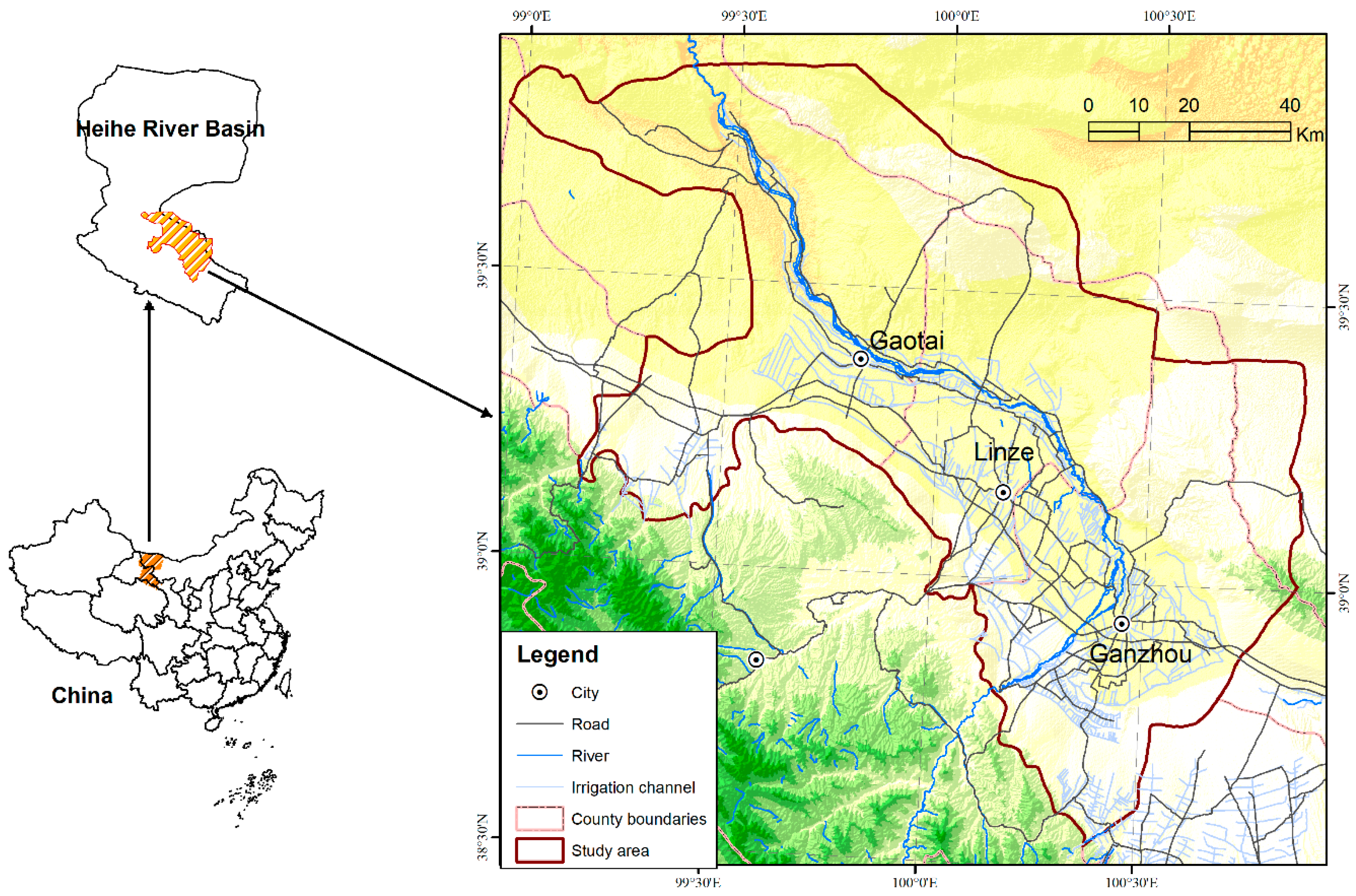
Zhangye Oasis was selected to simulate LUCC during 2000–2011. Zhangye Oasis belongs to Gansu Province, China, and is located in the midstream areas of the Heihe River Basin (HRB) (Figure 2). Its total area is 1.07 × 10⁴ km². The region is a typical irrigated agricultural oasis, and water resources are scarce. The water resources in this region are mainly from precipitation, snowmelt, and glacier melt in the Qilian Mountains. Water in the Heihe River is the determining factor for agricultural production and ecosystem stability. Major changes in land use patterns have occurred in Zhangye Oasis, driven by changes in the water environment and human activities over the past five decades [6]. In 2000, the Chinese Government implemented the Ecological Water Diversion Project (EWDP) to prevent further ecosystem deterioration and to restore the environment in the downstream areas of the HRB. In the framework of the EWDP, a “grain for green” policy (GGP) was implemented in Zhangye Oasis in 2002. Similarly, to restore wetlands along the Heihe River and to protect existing wetlands from being converted into cropland or built-up land, the Wetland Conservation Project (WCP) was also implemented in the midstream areas of the HRB in 2008. The agriculture and ecology in the Zhangye Oasis were subjected to these major water and environment policy changes. For example, wetland areas first decreased as a result of the pressure of the EWDP between 2000 and 2007, and then increased with the implementation of the WCP between 2007 and 2011 [27]. However, the most significant LUCC of this period in this region was still the substantial urban expansion and the continued reclamation of cropland, attributed to economic interests [27]. These changes increased the stress on water resources and the ecological environment. Therefore, potential risks are threatening the socio-economic and sustainable development.

3.1. Datasets

Spatial datasets were collected in order to build the proposed land use models and simulate the LUCC process (

Table 1. Spatial datasets for simulating multiple land use changes.

Category	Data	Calculation Method
Land use	Land use data (2000 and 2011)	Land use maps were generated using the visual interpretation method based on Landsat TM/ETM+ images.
Distance-based variables	Distance to town	The distance raster maps were generated using the distance analysis function of the Spatial Analysis module in ArcGIS. The distance data for each cell were read from the distance raster maps.
	Distance to village
	Distance to road
	Distance to river
	Distance to channel
Neighborhood conditions	Amount of cropland	$N\left(C_{mn},l\right)=\frac{{\displaystyle \sum _{i=m-1}^{m+1}{\displaystyle \sum _{j=n-1}^{n+1}clas{s}_{ij}}}}{9}$ where N(Cmn, l) is the effect of the lth type of land use on the center cell Cmn in the window, classij is the land use type in cell Cij. If the land use type in cell Cij is l, then classij = 1; otherwise classij = 0. The calculation of neighborhood effects was realized using Matlab.
	Amount of forestland
	Amount of grassland
	Amount of water body
	Amount of built-up land
	Amount of wetland
	Amount of desert
Topography	Elevation	DEM with 90 m resolution was come from the Shuttle Radar Topography Mission (SRTM) spearheaded by NASA and NIMA (ftp://e0mss21u.ecs.nasa.gov/srtm/). Slope and aspect data were extracted based on the DEM.
	Slope
	Aspect
Socio-economic	Population density	The population density with 25 m by 25 m resolution was obtained from the Environmental and Ecological Science Data Center for West China (http://westdc.westgis.ac.cn). The population data of each cell were read from the raster maps.

). Among these datasets, land use datasets were generated by employing the visual interpretation method based on 30 m resolution Landsat TM/ETM+ images in 2000 and 2011, which were downloaded from the U.S. Geological Survey (USGS) (http://glovis.usgs.gov/). The classification accuracies of land use types for 2000 and 2011 were greater than 90% [27]. Following the NLUD-C (National Land Use Database of China) classification system and land use characteristics in the study area, the classification system in this study included seven primary land use types: cropland, forestland, grassland, water body (referring to natural water bodies or lands with facilities for irrigation and water reservation), built-up land (including urban and rural settlements, factories, and transportation facilities), wetland, and desert (including sandy land, Gobi, saline, barren soil, and bare rock) [27,28]. Taking into account the requirements of data accuracy as well as the operational efficiency of the proposed models, the vector land use maps in 2000 and 2011 were separately converted into raster format with a resolution of 100 m × 100 m.

Other spatial datasets included distance-based variables, neighborhood conditions, socio-economic variables, and physical attributes (Table 1). Studies have also shown that the above driving variables are closely related to probabilities of land use changes [29,30,31]. Based on preliminary logistic regression analysis, these spatial driving variables were determined. These variables could well explain the spatial distributions of various land use types in the study (0.84 < the Relative Operating Characteristic value < 0.98). The raster maps for the distance-based variables, socio-economic variables, and physical attributes were generated with the Spatial Analysis module in ArcGIS. The raster maps of neighborhood influence were obtained through a standard 3 × 3 contiguity filter using Matlab software. All the spatial driving variables were unified to the same projection and resolution as the land use maps. Normalized values from 0 to 1 were then calculated using the maximum and minimum values after scaling the original spatial driving variable datasets.

3.2. Model Training

In order to train and compare the two proposed models, a pair of parallel simulations of LUCC in Zhangye Oasis during 2000–2011 were designed. Firstly, the annual transition probability matrix was obtained based on the actual historical development trend in the period 2000–2011, then the total amounts of various land use types were calculated using Markov chain. Secondly, model training was also essential before the simulation. The training data for the simulation period were extracted from the land use map in 2000 by a stratified random sampling technique which could reduce the spatial dependence of spatial data and avoid excessive data [23]. Each type of land use was sampled using a random sampling procedure, and a total of 56,000 random samples were selected. Simultaneously, the values of spatial driving variables were also obtained with randomly stratified sample points. In the MLRMCA model, calculation of the regression coefficients and creation of the logistic regression model were accomplished using these training data sets in SPSS software.

In the MANNMCA model, a three-layer ANN including the input layer, hidden layer, and output layer was used to simulate multiple land use change. There was a total of 17 spatial variables for each cell, and, consequently, there were 17 neurons in the input layer. In accordance with previous studies [13,32], the number of neurons in the hidden layer was at least 2n/3 (n is the number of neurons in the input layer). After many experiments, 12 neurons were used in the hidden layer. The 7 neurons in the output layer represented 7 types of land use. The training of the ANN was performed using the same sampling points based on a back-propagation (BP) algorithm. When a minimum mean square error was obtained, the training of the ANN stopped.

The regression coefficients and ANN weights obtained by training were imported into the MLRMCA and MANNMCA models, respectively, for simulation. The time interval for the simulation was one year. Each iteration represented a year. In each iteration, the transition probability of each land use type in each cell was calculated using the training model parameters mentioned above. According to the transition rules, and under the constraint of the total number of land use types, the land use patterns in the simulation period were simulated by the MLRMCA and MANNMCA models. It should be noted that the neighborhood influence was dynamically updated in the iteration loop in this study, unlike in previous studies [12,33].

3.3. Simulation Results

In order to assess the MLRMCA and MANNMCA model performances, their results were compared with the actual land use map in 2011.

Table 2. Observed and simulated land use change for 2000–2011 in the Zhangye Oasis.

Types	Actual Change		Simulated Change		Different between Simulated and Observed Change
	Number	Percentage	Number	Percentage	Number	Percentage
Cropland	25539	11.97%	24864	11.66%	−675	−0.32%
Forestland	962	7.16%	818	6.09%	−144	−1.07%
Grassland	−6926	−6.25%	−6514	−5.88%	412	0.37%
Water body	−1325	−8.61%	−1230	−7.99%	95	0.62%
Built-up land	3160	24.05%	3280	24.97%	120	0.91%
Wetland	−73	−0.46%	−79	−0.5%	−6	−0.04%
Desert	−21337	−3.11%	−21139	−3.08%	198	0.03%

Note: the percentage relates the amount of change to the total amount of land for a land use type in 2000.

showed that there was a strong agreement between the quantities of observed and simulated LUCC. All land use types had low relative errors, lower than 1.1%. The best agreement was shown in the desert type, where the actual area decreased by 3.11%, while the corresponding simulated area decreased by 3.08%. This showed that the developed Markov chain in this study could effectively simulate area change of land use.

The spatial accuracy of the simulation results was then analyzed quantitatively to evaluate the ability of the two models (

Table 3. Error matrix between actual land use and simulated result in 2011 (MLRMCA).

Actual Land Use in 2011	Simulated Land Use in 2011
	Cropland	Forestland	Grassland	Water Body	Built-Up Land	Wetland	Desert	Total	PA (%)
Cropland	213,635	2565	4681	631	2704	927	13,690	238,833	89.45
Forestland	1661	8252	1725	65	28	187	2477	14,395	57.33
Grassland	6015	1839	81,202	423	9	1177	13,158	103,823	78.21
Water Body	416	238	462	11,773	6	410	764	14,069	83.68
Built-Up Land	2168	17	43	3	13,610	15	442	16,298	83.51
Wetland	1363	34	571	538	40	12,291	841	15,678	78.40
Desert	12,900	1305	15,551	731	21	665	634,227	665,400	95.32
Total	238,158	14,205	104,235	14,164	16,418	15,672	665,599	1,068,496
UA (%)	89.70	57.91	77.90	83.12	82.90	78.43	95.29

Note: Overall accuracy = 91.25%; Kappa coefficient = 0.84; UA is user’s accuracy, and PA is producer’s accuracy; Bold numbers in diagonal are the correct simulations, and the off-diagonal numbers in rows and columns are errors.

and

Table 4. Error matrix between actual land use and simulated result in 2011 (MANNMCA).

Actual Land Use in 2011	Simulated Land Use in 2011
	Cropland	Forestland	Grassland	Water Body	Built-Up Land	Wetland	Desert	Total	PA (%)
Cropland	215,943	2997	2910	598	1781	844	13,760	238,833	90.42
Forestland	1492	9320	1503	66	73	66	1875	14,395	64.74
Grassland	5040	1262	85,984	418	468	1002	9649	103,823	82.82
Water Body	498	62	160	11,714	7	800	828	14,069	83.26
Built-Up Land	1991	9	17	3	13,687	51	540	16,298	83.98
Wetland	1708	68	190	687	43	11,643	1339	15,678	74.26
Desert	11,486	533	13,471	678	359	1266	637,607	665,400	95.82
Total	238,158	14,251	104,235	14,164	16,418	15,672	665,598	1,068,496
UA (%)	90.67	65.40	82.49	82.70	83.37	74.29	95.79

Note: Overall accuracy = 92.27%; Kappa coefficient = 0.86; UA is user’s accuracy, and PA is producer’s accuracy; Bold numbers in diagonal are the correct simulations, and the off-diagonal numbers in rows and columns are errors.

). For the MLRMCA model, the user’s and producer’s accuracies for cropland, water body, built-up land, and desert were greater than 80%, among which cropland and desert were highest. This meant that the spatial locations with those four types in the simulated map were relatively similar to those in the actual map. The over accuracy and the Kappa coefficient of the MLRMCA model were 91.25% and 0.84. For the MANNMCA model, the user’s and producer’s accuracies for the other five types in addition to forestland and wetland were also greater than 80%. The over accuracy and the Kappa coefficient were 92.27% and 0.86, respectively. These results indicated that although a certain bias was exhibited, more similarities were found between the simulated results of the two models and the actual map. Figure 3 also indicated that the spatial distribution of various land use types simulated by the two models were similar to the actual, especially in farmland and desert types. However, there were still some discrepancies in the simulated maps. For example, in the north of the Ganzhou District, some small wetland patches were not simulated by the two proposed models.

It must be mentioned, however, that Kappa coefficient was an indication of the location agreement between observed and simulated land use. This may lead to an overestimation of the model performance when the area of the LUCC was relatively small. So, this study further analyzed the LUCC between observation and simulation by pixel-by-pixel comparison. Figure 4 showed that the area of LUCC in Zhangye Oasis was relatively small, accounting for only about 6% of the total area. This is mainly due to the fact that desert was the largest type of land use in the study area, the landscape pattern of which is relatively stable and difficult to exploit and utilize. Thus, the FM values of the two models proposed by this study were both relatively low (

Table 5. Figure of merit (FM) for simulated land use change (%).

Model	Cropland	Forestland	Grassland	Water Body	Built-Up Land	Wetland	Desert	Overall
MLRMCA	32.17	4.06	2.12	0.00	14.44	3.40	1.43	12.56
MANNMCA	32.93	1.22	21.51	0.85	16.79	3.89	20.04	22.32

). For the MLRMCA model, the FM values for cropland and built-up land were highest, at 32.17% and 14.44%, respectively. The FM for water body was lowest. The overall FM of the MLRMCA model was 12.56%. Similarly, for the MANNMCA model, the FM values for cropland and grassland were highest, at 32.93% and 21.54%, respectively. The FM for water body was also lowest, at 0.85%. The overall FM of the MANNMCA model was 22.32%. This result revealed that the ability of the two models to simulate changes was best for cropland, and lowest for water bodies.

The above results show that the accuracies of the amounts and spatial distributions of the two proposed models were both satisfactory. Therefore, the two proposed models were both able to simulate and predict future land use evolution processes.

3.4. Model Validation and Comparison

In order to validate the advantages and disadvantages of the two proposed models, the simulation results of the MLRMCA model were compared with those of the MANNMCA model. Figure 3 shows that the development direction of built-up land in the center of Ganzhou District and the landscape pattern of grassland in the north desert area of the oasis simulated by the MLRMCA model were better than those simulated by the MANNMCA model, and were closer to those in the true land use map. However, on the edge of the oasis, the expansion trend in cropland simulated by the MANNMCA model was closer to that of the true map. For example, on the eastern edge of the oasis, the actual amount of cropland had increased by 40.39% during 2000–2011, while the increases simulated by the MLRMCA and MANNMCA models were 10.13% and 29.38%, respectively. In addition, the simulation results of the MLRMCA and MANNMCA models also showed little difference in the region for well-predicted change (Figure 4). The region for well-predicted change simulated by the MLRMCA model was mainly located in the oasis. However, in addition to the internal distribution of the oasis, the region for well-predicted change simulated by the MANNMCA model was located on the edge of the oasis, the northwest corner, the western margin, and the northeast corner of the oasis.

From the accuracy of the simulation results (Table 2, Table 3, Table 4 and Table 5), the amounts of all land use types which were simulated based on the same historical data by Markov chain were the same in the MLRMCA model and MANNCA model, and were close to the actual number in the simulation period. In terms of spatial accuracy, the Kappa coefficients and the overall FM value in the MANNMCA model were all higher than those of the MLRMCA model. The user’s and produce’s accuracies for another four types in addition to water body and wetland in the MANNMCA model were higher than those in the MLRMCA model. In addition to forestland, FM values for the other six land use types in the MANNMCA model were higher than those in the MLRMCA model.

In short, the MANNMCA model showed relatively considerable improvement over the MLRMCA model in terms of spatial accuracy. However, the MLRMCA model was better than the MANNMCA model in terms of the spatial distribution in water body and wetland, and the temporal change trends in forestland.

4. Discussion and Conclusions

This paper proposed two integrated CA models which combined Markov Chain and Logistic Regression, and Markov Chain and ANN, respectively, into a multiple CA model to simulate a complex and nonlinear land use evolutionary process. Compared with the traditional CA model, the two integrated CA models not only took advantage of the Markov Chain for quantitative forecasting and the CA model for simulating the spatial distribution of a complex system, but also employed a full Logistic Regression and ANN model for determining the parameter values. On the other hand, according to the characteristics of agricultural development in this arid oasis, the two CA models considered the impact of artificial irrigation on the spatial pattern of land use, different from the previous studies of CA models [34,35]. Therefore, the two integrated models can help improve the analysis and prediction of LUCC.

The proposed two models were used in the simulation of land use patterns in Zhangye Oasis, Gansu Province, China. The performances of the MLRMCA and MANNMCA models were evaluated and compared using user’s and produce’s accuracies, Kappa coefficient, and FM indices. Overall, the simulated maps showed better agreement with the corresponding observation data. The MANNMCA model generally performed better than the MLRMCA model. However, the MLRMCA model also showed some advantages over the MANNMCA model simulation. Differences between the two proposed model performances were attributed to the differences in summarizing the complex relationships between the transition probabilities of land use types and a set of spatial driving variables in the calibration phase. The simulation accuracy for the CA model was largely influenced by the weight value of the spatial variable. The MANNMCA model can generate more accurate model parameters than linear approaches (MLRMCA model). This is because the ANN was able to capture nonlinear complex features, although the “black box” operation of the ANN made the physical meaning of the model parameters unclear. The MLRMCA model yielded a slightly lower simulation accuracy because the logistic regression approach obscured the autocorrelation of the spatial variables. However, the logistic regression approach could identify possible driving factors responsible for LUCC.

The FM value for water body in the two models was lowest compared with those for the other six land use types. The reason for this was that the river was used as a constraint factor in the two models, which limited the conversion of other types to water body. In addition, the user’s and producer’s accuracies for forestland and wetland in the two models were lower. One reason for this could be that the patches of forestland and wetland were small and scattered. The second reason for this was the original data classification accuracy and the rate of change of the original land use types, which could affect both the inputs and outputs of both models. The final reason might be the implementation of the water and environment policies (e.g., EWDP, GGP, and WCP), which was not included in this study but should be considered in the future. These factors made it difficult for both models to simulate this complex pattern.

Although there are some limitations, the two proposed models can meet the needs of simulating and predicting regional LUCC trends, and can also provide a reference for water resource assessment, ecological restoration, and sustainable urban development in arid areas.

References

- Lambin, E.F.; Turner, B.L.; Geist, H.J.; Agbola, S.B.; Angelsen, A.; Bruce, J.W.; Coomes, O.T.; Dirzo, R.; Fischer, G.; Folke, C.; et al. The causes of land-use and land-cover change: Moving beyond the myths. Glob. Environ. Chang. 2001, 11, 261–269. [Google Scholar] [CrossRef]
- Turner, B.L.; Lambin, E.F.; Reenberg, A. The emergence of land change science for global environmental change and sustainability. Proc. Natl. Acad. Sci. USA 2007, 104, 20666–20671. [Google Scholar] [CrossRef] [PubMed] [Green Version]
- Mahmood, R.; Pielke, R.A.; Hubbard, K.G.; Niyogi, D.; Dirmeyer, P.A.; McAlpine, C.; Carleton, A.M.; Hale, R.; Gameda, S.; Beltrán-Przekurat, A.; et al. Land cover changes and their biogeophysical effects on climate. Int. J. Climatol. 2014, 34, 929–953. [Google Scholar] [CrossRef]
- Borrelli, P.; Robinson, D.A.; Fleischer, L.R.; Lugato, E.; Ballabio, C.; Alewell, C.; Meusburger, K.; Modugno, S.; Schütt, B.; Ferro, V.; et al. An assessment of the global impact of 21st century land use change on soil erosion. Nat. Commun. 2017, 8, 2013. [Google Scholar] [CrossRef] [PubMed] [Green Version]
- Newbold, T.; Hudson, L.N.; Hill, S.L.; Contu, S.; Lysenko, I.; Senior, R.A.; Börger, L.; Bennett, D.J.; Choimes, A.; Collen, B.; et al. Global effects of land use on local terrestrial biodiversity. Nature 2015, 520, 45–50. [Google Scholar] [CrossRef] [PubMed] [Green Version]
- Cheng, G.D.; Li, X.; Zhao, W.Z.; Xu, Z.M.; Feng, Q.; Xiao, S.C.; Xiao, H.L. Integrated study of the water-ecosystem-economy in the Heihe River Basin. Nat. Sci. Rev. 2014, 1, 413–428. [Google Scholar] [CrossRef]
- Li, X.; Cheng, G.D.; Kang, E.S.; Xu, Z.M.; Nan, Z.T.; Zhou, J.; Han, X.J.; Wang, S.G. Digtial Heihe River Basin. 3: Model Integration. Adv. Earth Sci. 2010, 25, 851–865. (In Chinese) [Google Scholar]
- Li, X.; Cheng, G.D.; Lin, H.; Cai, X.M.; Fang, M.; Ge, Y.C.; Hu, X.L.; Chen, M.; Li, W.Y. Watershed system model: The essentials to model complex human-nature system at the river basin scale. J. Geophys. Res. Atmos. 2018, 123, 3019–3034. [Google Scholar] [CrossRef]
- Marcucci, D.J. Landscape history as a planning tool. Landsc. Urban Plan. 2000, 49, 67–81. [Google Scholar] [CrossRef]
- Verburg, P.H.; Schot, P.P.; Dijst, M.J.; Veldkamp, A. Land use change modeling: Current practice and research priorities. GeoJournal 2004, 61, 309–324. [Google Scholar] [CrossRef]
- Wu, F.; Webster, C.J. Simulation of land development through the integration of cellular automata and multicriteria evaluation. Environ. Plan. B 1998, 25, 103–126. [Google Scholar] [CrossRef]
- Wu, F. Calibration of stochastic cellular automata: The application to rural-urban land conversions. Int. J. Geogr. Inf. Sci. 2002, 16, 795–818. [Google Scholar] [CrossRef]
- Li, X.; Yeh, A.G.O. Neural-network-based cellular automata for simulating multiple land use change using GIS. Int. J. Geogr. Inf. Sci. 2002, 16, 323–343. [Google Scholar] [CrossRef]
- Yassemi, S.; Dragićević, S.; Schmidt, M. Design and implementation of an integrated GIS-based cellular automata model to characterize forest fire behavior. Ecol. Model. 2008, 210, 71–84. [Google Scholar] [CrossRef]
- Yang, Q.S.; Li, X. Calibration urban cellular automata using genetic algorithms. Geogr. Res. 2007, 26, 229–237. (In Chinese) [Google Scholar]
- Arsanjani, J.J.; Helbich, M.; Kainz, W.; Boloorani, A.D. Integration of logistic regression, Markov chain and cellular automata models to simulate urban expansion. Int. J. Appl. Earth Obs. 2013, 21, 265–275. [Google Scholar] [CrossRef]
- Han, H.R.; Yang, C.F.; Song, J.P. Scenario simulation and the prediction of land use and land cover change in Beijing, China. Sustainability 2015, 7, 4260–4279. [Google Scholar] [CrossRef]
- Zhang, H.; Zhang, B.; Verburg, P. The Future variations of land use and land coverage in arid regions, Modeled in three scenarios of water resources. J. Glaciol. Geocryol. 2007, 29, 397–405. (In Chinese) [Google Scholar]
- Cao, X.; Luo, P.; Li, M.C.; Li, H.G.; Long, A.H. Spatio-temporal simulation of land use change based on a extended CA model: A case study of Shenzhen city, China. Resour. Sci. 2011, 33, 127–133. (In Chinese) [Google Scholar]
- Veldkamp, A.; Lambin, E.F. Prediction land-use change. Agric. Ecosyst. Environ. 2001, 85, 1–6. [Google Scholar] [CrossRef]
- Weng, Q.H. Land use change analysis in the Zhujiang Delta of China using satellite remote sensing, GIS and stochastic modelling. J. Environ. Manag. 2002, 64, 273–284. [Google Scholar] [CrossRef] [Green Version]
- Serneels, S.; Lambin, E.F. Proximate causes of land use change in Narok district Kenya: A spatial statistical model. Agric. Ecosyst. Environ. 2001, 85, 65–82. [Google Scholar] [CrossRef]
- Xie, C.; Huang, B.; Claramunt, C.; Chandramouli, M. Spatial logistic regression and GIS to model rural-urban land conversion. In Proceedings of the PROCESSUS Second International Colloquium on the Behavioural Foundations of Integrated Land-use and Transportation Models: Frameworks, Models and Applications, University of Toronto, Toronto, ON, Canada, 12–15 June 2005. [Google Scholar]
- Viera, A.J.; Garrett, J.M. Understanding interobserver agreement: The kappa statistic. Fam. Med. 2005, 37, 360–363. [Google Scholar] [PubMed]
- Koomen, E.; Diogo, V.; Hilferink, M.; Van der Beek, M.C.J. EuClueScanner100m Model Description and Validation Results; European Commission JRC: Brussels, Belgium, 2010. [Google Scholar]
- Pontius, R.G.; Boersma, W.; Castella, J.C.; Clarke, K.; de Nijs, T.; Dietzel, C.; Duan, Z.; Fotsing, E.; Goldstein, N.; Kok, K.; et al. Comparing the input, output, and validation maps for several models of land change. Ann. Reg. Sci. 2008, 42, 11–37. [Google Scholar] [CrossRef]
- Hu, X.L.; Lu, L.; Li, X.; Wang, J.H.; Guo, M. Land use/cover change in the middle reaches of the Heihe River Basin over 2000–2011 and its implications for sustainable water resource management. PLoS ONE 2015, 10, e0128960. [Google Scholar] [CrossRef] [PubMed]
- Liu, J.Y.; Liu, M.L.; Tian, H.Q.; Zhuang, D.F.; Zhang, Z.X.; Zhang, W.; Tang, X.M.; Deng, X.Z. Spatial and temporal patterns of China’s cropland during 1990–2000: An analysis based on Landsat TM data. Remote Sens. Environ. 2005, 98, 442–456. [Google Scholar] [CrossRef]
- Li, X.; Yeh, A.G.O. Modelling sustainable urban development by the integration of constrained cellular automata and GIS. Int. J. Geogr. Inf. Sci. 2000, 14, 131–152. [Google Scholar] [CrossRef] [Green Version]
- Li, Y.C.; He, C.Y. Scenario simulation and forecast of land use/cover in northern China. Chin. Sci. Bull. 2008, 53, 1401–1412. [Google Scholar] [CrossRef]
- Liu, X.P.; Li, X.; Zhang, X.H.; Chen, G.Q.; Li, S.Y.; Chen, Y.M. Embedding urban planning objective by integrated artificial immune system and cellular automata. Acta Geogr. Sin. 2008, 63, 882–894. (In Chinese) [Google Scholar]
- Wang, F. The use of artificial neural networks in a geographical information system for agricultural land-suitability assessment. Environ. Plan. A 1994, 26, 265–284. [Google Scholar] [CrossRef]
- Guan, D.J.; Li, H.F.; Inohae, T.; Su, W.C.; Nagaie, T.; Hokao, K. Modeling urban land use change by the integration of cellular automaton and Markov model. Ecol. Model. 2011, 222, 3761–3772. [Google Scholar] [CrossRef]
- Clarke, K.C.; Hoppen, S.; Gaydos, L. A self-modifying cellular automaton model of historical urbanization in the San Francisco Bay area. Environ. Plan. B 1997, 24, 247–261. [Google Scholar] [CrossRef] [Green Version]
- Dietzel, C.; Clarke, K. The effect of disaggregating land use categories in cellular automata during model calibration and forecasting. Comput. Environ. Urban 2006, 30, 78–101. [Google Scholar] [CrossRef]
Figure 1.
Structure of the multiple logistic regression cellular automata (MLRMCA) model and the multiple artificial neural network cellular automata (MANNMCA) model.
Figure 2.
Location of the study area.
Figure 3.
Simulated land use maps by MLRMCA and MANNMCA models and observed land use maps for 2007 and 2011.
Figure 4.
Three-map comparison for simulated and observed land use change in Zhangye Oasis between 2000 and 2011.