Article

A Machine Learning Approach to the Residential Relocation Distance of Households in the Seoul Metropolitan Region

1
Department of Urban Engineering, Hanbat National University, Daejeon 34158, Korea
2
Department of Urban Planning and Design, University of Seoul, Seoul 02504, Korea
*
Author to whom correspondence should be addressed.
Sustainability 2018, 10(9), 2996; https://doi.org/10.3390/su10092996
Submission received: 23 July 2018 / Revised: 21 August 2018 / Accepted: 21 August 2018 / Published: 23 August 2018

Abstract

:
This study aimed to evaluate the applicability of a machine learning approach to the description of residential mobility patterns of households in the Seoul metropolitan region (SMR). The spatial range and temporal scope of the empirical study were set to 2015 to review the most recent residential mobility patterns in the SMR. The analysis data used in this study included the Internal Migration Statistics microdata provided by the Microdata Integrated Service of Statistics Korea. We analysed the residential relocation distance of households in the SMR using machine learning techniques, such as ordinary least squares regression and decision tree regression. The results of this study showed that a decision tree model can be more advantageous than ordinary least squares regression in terms of explanatory power and estimation of moving distance. A large number of residential movements are mainly related to the accessibility to employment markets and some household characteristics. The shortest movements occur when households with two or more members move into densely populated districts. In contrast, job-based residential movements are relatively farther. Furthermore, we derived knowledge on residential relocation distance, which can provide significant information for the urban management of metropolitan residential districts and the construction of reasonable housing policies.

1. Introduction

Although some people continue their lives in only one location, a large number of households experience multiple residential movements during their existence. Residential movements have been studied in terms of residential choices and preferences as a searching process for the appropriate location and dwelling with respect to individual characteristics. However, residential choices and preferences should be clearly distinguished. Residential choices indicate the actual behaviour related to residential movement, and residential preference is related to the relative attractiveness of housing and residential environment that affect movers [1]. Residential mobility can be represented by the spatial movement pattern based on actual behaviours of the movers. Previous studies of spatial patterns of residential relocations focused on the conventional research topics: frequency, direction, and distance of residential mobility. The life-cycle model [2], sector model [3], and Ravenstein’s Laws [4] are representative research achievements, as well as the theories related to these subjects. However, the relevant empirical studies for household units have paid relatively scant attention to the topics of direction and distance of residential mobility. This could be due to the excessive complexity of influencing factors, lack of computing power to handle large volumes of data on household movements, and absence of an appropriate analytical model [5].
After economic achievement and quantitative growth [6], the Korean housing market has experienced structural changes in terms of both supply and demand. The housing shortage problem of Korean society was considered to have been resolved with the housing supply ratio exceeding 100% in the early 21st century. A fundamental change in the nature of the household [2], which is a basic unit of residential mobility and location change, is in progress. Representative phenomena include the reduction in the household size and aging, indicating the emergence of a new demand class and the change in characteristics in the core demand groups. These situations are summarised as the transitioning from a supply-based housing market to a demand-driven market [7]. Regarding the demand, with the slowdown in population growth, the flow management of residential mobility, considering the relocations within the metropolitan region, is becoming more important than the response to new demand caused by increased population in the metropolitan region. Previous studies [8,9] confirmed that the frequency of residential relocations of Korean households is relatively high among the Organization for Economic Cooperation and Development (OECD) countries. In addition, recent studies [10,11] have shown that residential relocation distance could be differentiated by household size and age of householder in the Seoul metropolitan region (SMR), which is the most representative and largest metropolitan region in Korea. These phenomena could be changed by the reduction in household size and aging trends.
An empirical understanding of spatial patterns and characteristics related to residential relocation is important for the establishment of an in-depth housing policy. In addition, considering the growing socio-economic complexity, residential mobility research using spatial Big Data is more advantageous than research using only aggregated data. Study based on actual moving data of households are more meaningful, as they can identify the practical residential moving patterns, considering the conditions of a household rather than the ideal pursuit of a specific household. In a continually changing housing market, such as the Korean housing market, the outcomes of such a study could be applied to build a simulation model for forecasting future residential relocations. Accordingly, academic reviews and empirical studies must attempt to apply new analytical methods, such as machine learning, which is used to derive meaningful knowledge from Big Data in the housing and residential research fields, among others. If such an attempt is successful, in the long run, the model could be used to construct a sustainable housing-market management system because a machine learning model focuses more on predictive power than a conventional statistical model.
In this context, this study aimed to ascertain the applicability of a machine learning approach based on spatial Big Data converted from the available microdata related to household residential relocations to the description of the residential mobility patterns of households in the SMR. In particular, this study focuses on the residential relocation distances of households, which is one of the main topics representing residential spatial patterns, which has not been a focus of previous empirical studies on household units. Notably, residential relocation distance is a key factor in determining the spatial extent of the housing (sub)market. In this paper, we first review literature on patterns and influencing factors of residential relocation and examine the relocation characteristics of the SMR in Korea. Next, we conduct empirical studies analysing the determinants in residential relocation distance by using a machine learning approach. Finally, we conclude by summarising the outcomes of this study and ascertaining the applicability of the machine learning method in estimating or forecasting studies of housing and residential research.

2. Literature Review

Residential mobility is defined as a process of adjusting location to better meet the needs and demands of a household [7,12,13]. Residential mobility can be divided into residential relocation and urban migration. Residential relocation implies moving a residence within an urban living region, and urban migration can be defined as interregional movements. Whereas urban migration mostly results from changes in urbanisation and industrial structure [14], residential relocation is influenced by internal and external factors of a household, such as income, composition, housing preference, and residential environments. Residential movement occurs based not only on dissatisfaction with current location, but also attractiveness to the new location [15,16,17]. Previous studies, which examined the influencing factors of residential mobility, assumed a household-based decision-making mechanism. These representative studies considered various household characteristics, such as composition of household members [18], age and income [19], education level [20], and marriage duration [21]. However, these studies mainly focused on analysing residential mobility.
Recently, not only the amount of flow but also the residential mobility patterns have received interest in terms of suggesting implications for spatial planning and housing policy [11,22,23,24,25]. The moving patterns of households can be explained using the frequency, direction, and distance of residential mobility. In terms of the frequency of residential movement, the main reasons for residential mobility are the characteristics of the household and the changes in the life cycle of the household. The household life cycle is a series of processes that human beings experience in their lives, resulting in a change in needs and demands for the living space according to each stage [2,26,27]. According to the life cycle model, the changes in the characteristics of the frequency of movements depend on family events, such as marriage (formation), birth of children (expansion), moving out (contraction), and divorce or death of a spouse (dissolution) [2]. As the characteristics of the household change according to the life cycle stage, many researchers studied the probability of residential mobility affected by a particular stage. Previous studies showed various empirical results in consideration of birth, childcare, marital age, and income with respect to individual households [18,19,20,21,26,28,29].
In terms of residential mobility direction, Hoyt’s sector theory, which states, “High grade residential growth tends to proceed from the given point of origin, along established lines of travel or toward another existing nucleus of buildings or trading centres” [3], was the initial theory in this research field. This theory suggests that the direction of residential mobility is due to the difference in the rent generated in urban space. In an empirical study related to this theory, Burnley et al. [30] found that most of the residential mobility in Australia is biased outward from urban centres. Furthermore, Yang [31] reported that 26% of households moved to the outskirts of the city from the urban centre, whereas only 9% of the households moved in the opposite direction. Regarding the distance of residential movement, the widely known Ravenstein’s Laws suggests that most migration occurs over short distances [4]. The main research topics covered by related studies were concentrated on the quantity of flow of residential movement between origin and destination, based on the gravity model. That is, the results of previous studies highlighted the lack of in-depth research on the spatial patterns of residential moving distance. The short distance of residential movements is related to the existence of local housing markets (or housing submarkets) [32]. This study is a basic model that explains the residential relocation distance and links residential mobility to the local housing market. However, these previous studies did not consider the demographic and socio-economic changes of modern society. In addition, whereas the studies on the frequency of residential movement considered the various characteristics of households, some studies on residential relocation distance and moving direction only considered the household characteristics.
Several studies determined that the residential relocation distance differs according to household size, home ownership, job change, and parental status [10,11,29,33]. However, these studies compared and analysed the residential moving data aggregated by household characteristic. Recently, some literature focused on determinants affecting the residential relocation distance of households using spatial microdata. Such studies showed that demographic and socio-economic characteristics of households could affect the distance [34,35] and pointed to the limitation of aggregated residential moving distance data [36]. Nevertheless, a model for estimating the moving distance of each household has not yet been developed. This is mostly due to the difficulty in obtaining the data of moved households and the lack of an analytical method for large volume data [5]. Nowadays, a large amount of residential relocation data of individual households is being provided by the Korean government agency and various analysing methods are being developed for Big Data. Especially in the Korean housing market, which is experiencing a rapid demographic change, understanding the spatial patterns of residential movements is gaining increasing importance due to the housing demand and the behaviour of housing movement gradually changing based on the household type. Therefore, this study focused on the application of a new approach that uses machine learning, which is advantageous for Big Data analysis, in order to empirically identify the impact of the household attributes and the location characteristics on the residential relocation distance in Korea.

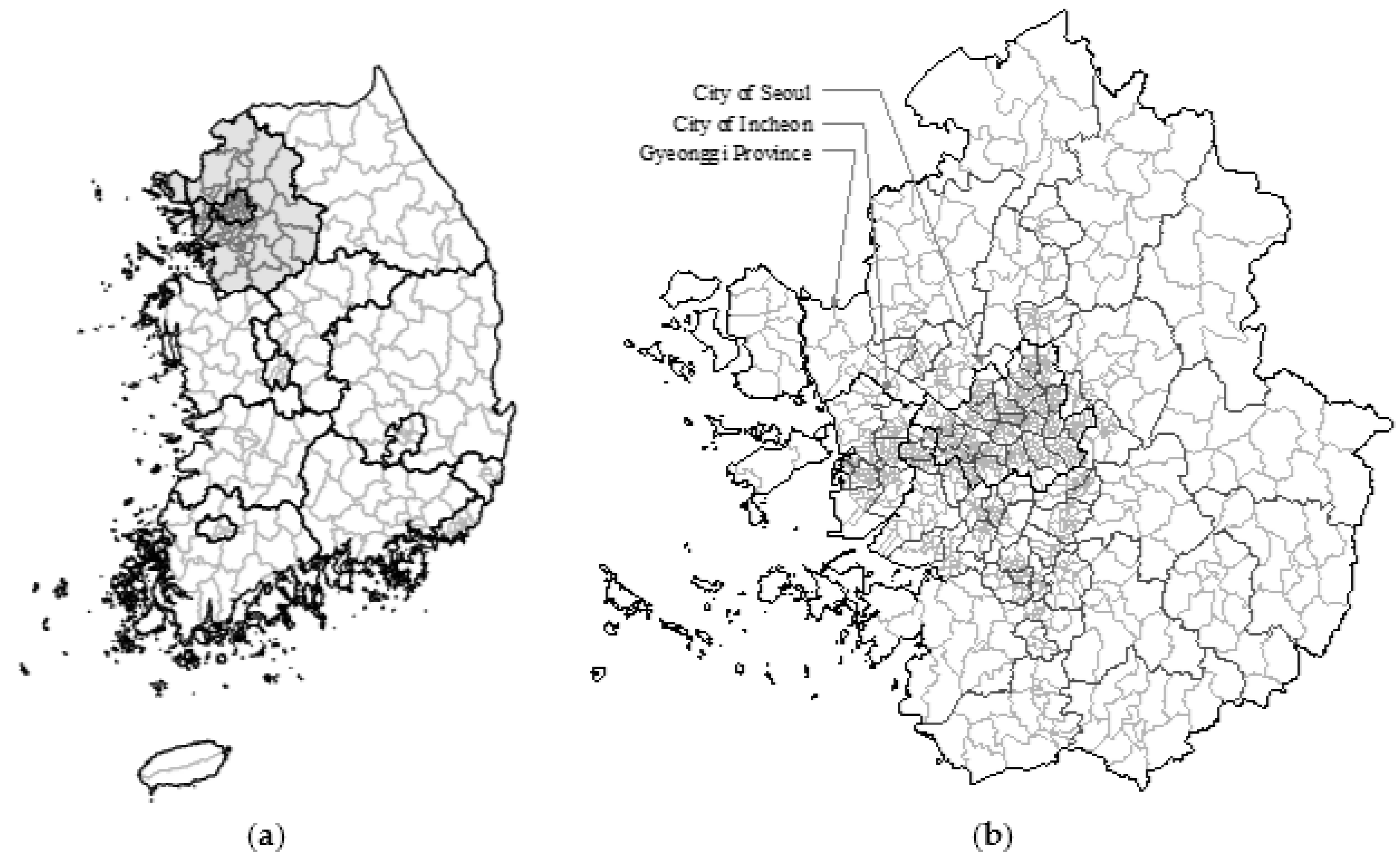
3. Characteristics of Residential Relocation Distance in SMR

The main spatial range of this study was the SMR, which is a representative metropolitan region of South Korea in terms of political, social, and cultural leadership, as well as population and economic scales, located in the northwestern part. The temporal scope was the year 2015. The spatial unit of the present empirical analysis involved the administrative district (Eup, Myeon, and Dong), which is a minimum-sized administrative-area-level unit in the SMR. The total area of the SMR is 11,828 km2, with a population of 23.906 million people living in 9.519 million households. In addition, the SMR contains two metropolitan cities (Seoul and Incheon), one province (Gyeonggi-do), 28 cities (Si), 5 counties (Gun), and 53 boroughs (Gu), which comprise 1,133 small administrative areas (Eup, Myeon, and Dong) (Figure 1 and Table 1).
The microdata from the Internal Migration Statistics of Korea were used to analyse the spatial characteristics of residential relocation. Internal Migration Statistics include information about Korean migrants to/from the smallest administrative areas of Eup, Myeon, and Dong obtained by using the migrant’s moving-in notifications. First, in the data collected in 2015, the total number of residential movements of households in Korea exceeded 6 million (6,098,915), of which approximately 3.1 million occurred in the SMR. The share of residential relocations within the SMR was 88.4%, which represented the majority of residential mobility in the metropolitan region. The share of residential mobility in the metropolitan region was differentiated from the movement toward the inside and outside by the municipality. The rates of residential relocations within the area were relatively low in the metropolitan cities, such as Seoul and Incheon, and approximately 30% of residential movement was confirmed to be beyond the boundaries of each municipality. The number of residential movements per household was 0.326 in 2015, and the difference by area was not significant. Second, the average residential relocation distance was 9.123 km in the SMR. As expected, the average distance of residential movement from Seoul was the shortest (7.753 km), and that from Gyeonggi province was the longest (10.391 km). However, moving-out beyond the boundary of Incheon city, with the longest distance (29.112 km), was an unexpected outcome. This result was presumed to be caused by the difference in the characteristics of the moving-out households (Table 2).
Figure 2 shows the difference among residential moving distance by household types according to characteristics of the household. In terms of household size, households with more members moved shorter distances. The households with three or more people in the metropolitan cities (Seoul and Incheon) moved a similar distance, whereas the relocation distance of one-person households showed a significant difference among municipalities. In addition, the age of a householder is considered a critical factor affecting the residential relocation distance of households, and this result is identical to previously confirmed outcomes. The longest relocation distance of households occurs for householders under age 30, and decreases in the age range of 40 to 49. Then, the distance of residential movement gradually increases with age. This phenomenon agrees with the previously reported results in Korea [10,11].
The estimated results of residential relocation distance in the SMR has several implications. First, the moving distance with respect to a household could vary according to the area in which the household is located. Second, depending on the characteristics of the household members, there could be differences in the moving distance. These outcomes imply that characteristics of households and their location features should be considered in the construction of an empirical model for ascertaining the applicability of a machine learning approach related to estimation of residential relocation distance. The effects of the characteristics of households and location features on household residential relocation distance will be identified and interpreted in more detail in the empirical analysis in the following section.

4. Materials and Methods

The research question of this empirical analysis is whether a machine learning approach can be applied to residential mobile pattern analysis. To this end, the following empirical analysis models and data were used.

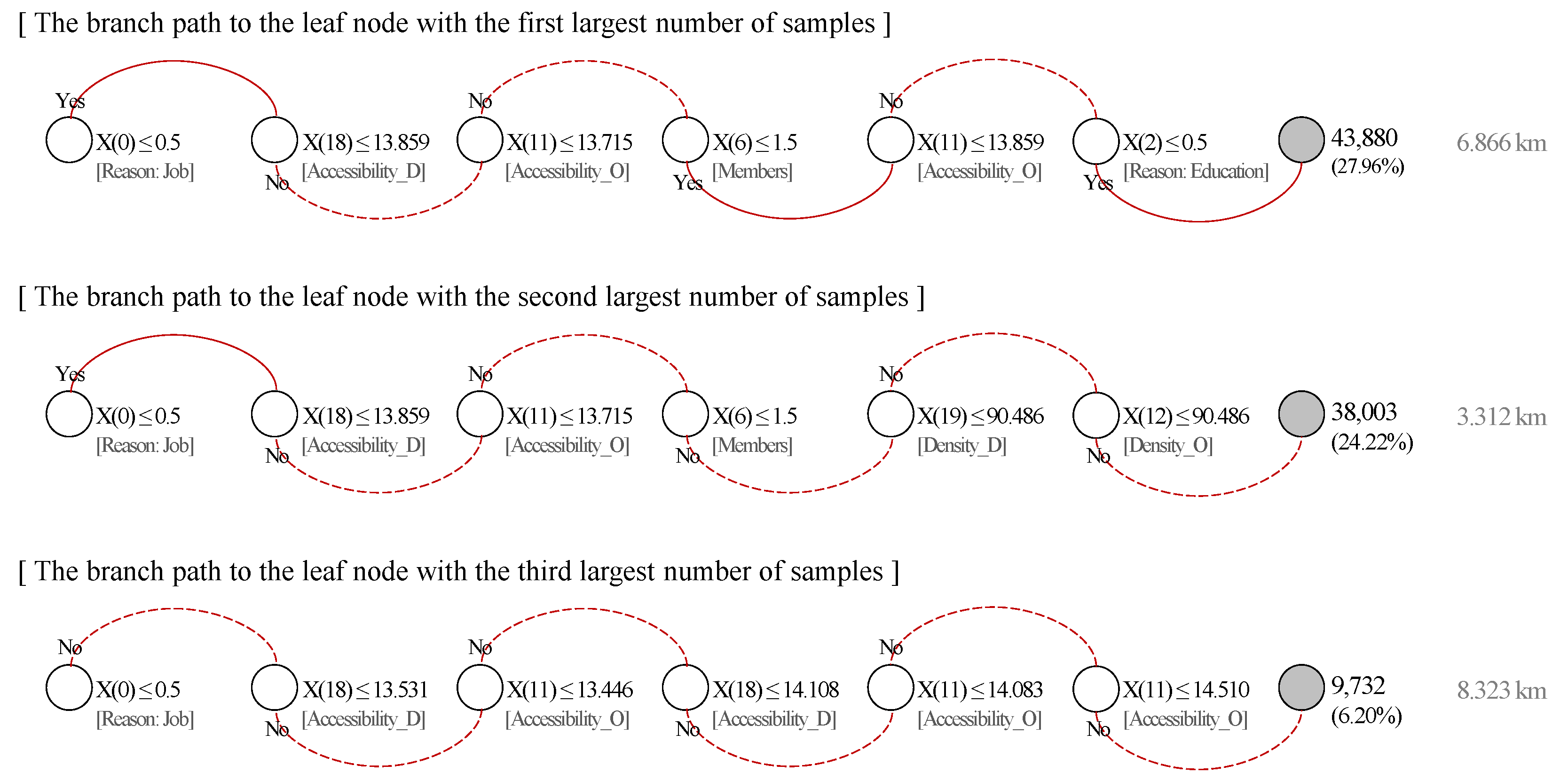
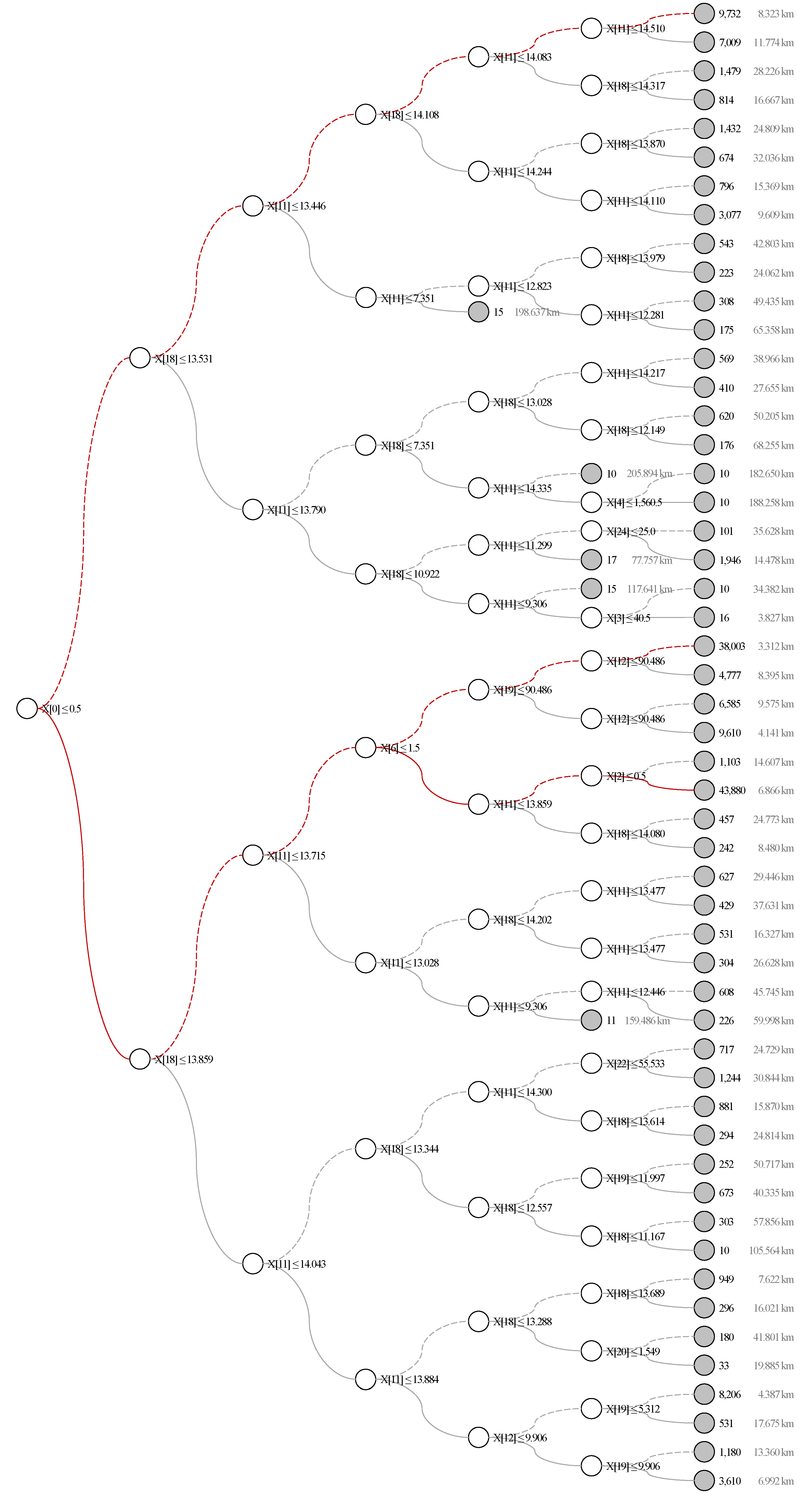
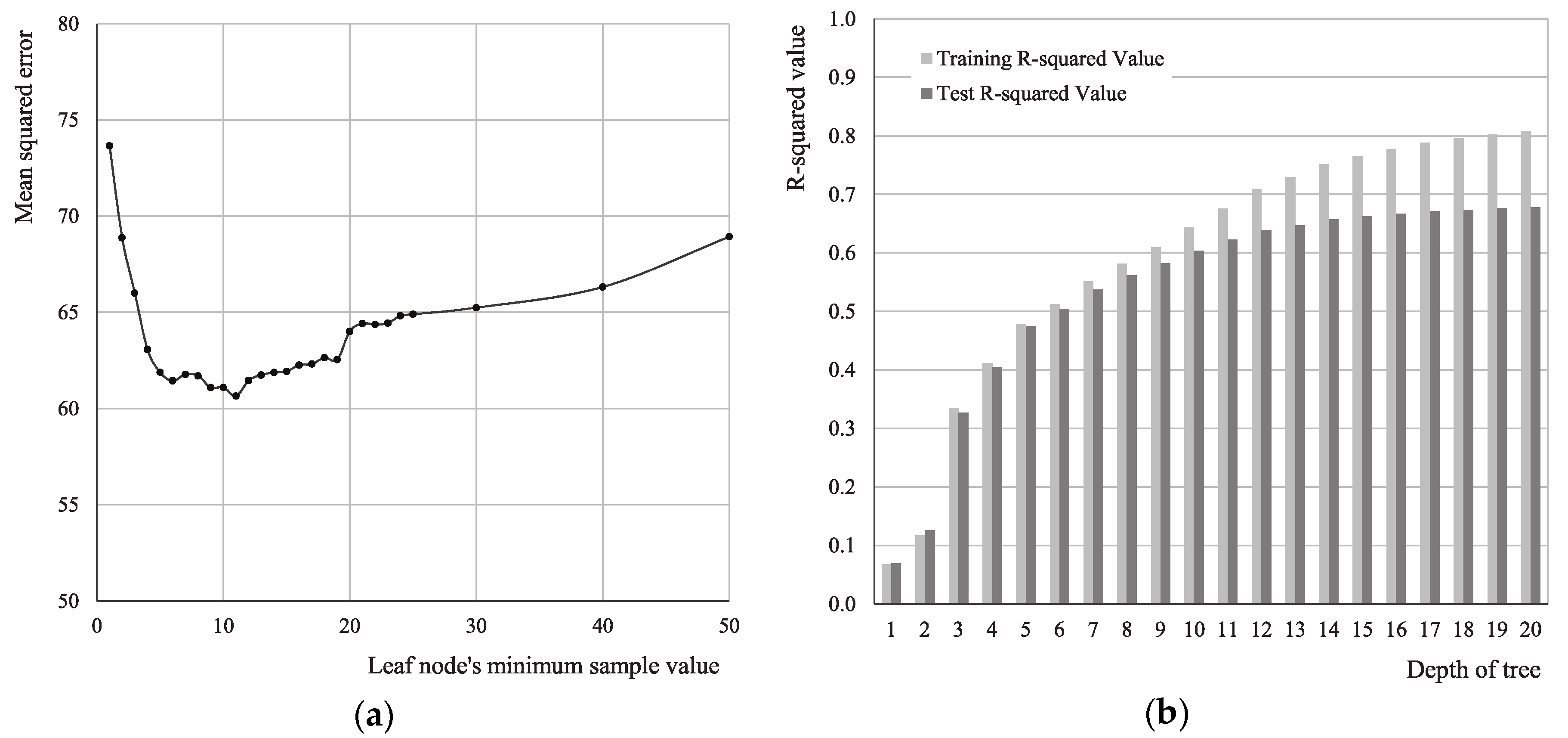
4.1. Decision Tree Using Machine Learning

The main analytical methodology of this study was machine learning, which is an efficient tool for automatically detecting patterns of data and extracting information from large datasets [37]. Machine learning differs from conventional statistics in that it is more focused on making estimations or predictions using a model, and formulating the generalisation process as a search through hypotheses. In contrast, conventional statistics are more concerned with testing hypotheses [38]. Machine learning focuses on estimation or prediction by considering an optimal model, whereas the latter concentrates on understanding the relationships between data. Recently, a few related studies applying a machine learning-based method have been reported in various research fields, such as environmental science, geomatics, and social science [39,40,41,42].
Decision trees in machine learning techniques are widely used for classification or regression problems. They generate the result in a tree form, which can be interpreted relatively easily compared to the results of other techniques [43,44]. Thus, decision trees are known as a white-box model in the software engineering field. Decision trees are classified into classification and regression trees, which are constructed by repeatedly splitting data. Each branch of a regression tree is partitioned according to the homogeneity of two resulting groups; the homogeneity is maximised according to the response variable. This method does not assume a relationship between the response and predictors, unlike the conventional statistical model in which the independent and dependent relationship variables are predefined and verified [45]. Therefore, the decision-tree regression method has more advantages than the conventional statistical models with respect to fitting and estimation using extremely complex data and structures. Therefore, in this study, the residential relocation distance of each household in the SMR was analysed using decision-tree regression, which can be regarded as the most appropriate model for analysis and estimation, considering rapidly changing demographic transitions and household characteristics in the Korean housing market.

4.2. Selection of Explanatory Variables and Generation of Analysing Data

The estimated residential relocation distance was the dependent variable for conducting empirical analysis using a decision tree. The microdata obtained from the Internal Migration Statistics in this study provided information about the smallest administrative district (Eup, Myeon, and Dong), which is the same as a small-sized traffic analysis zone (TAZ), for the point of departure and destination of each household’s residential movement. Therefore, we estimated the moving distance between the departure and destination based on the administrative centre points by applying the Euclidian distance calculation method. The cases for which the point of departure and destination were the same, the following formula was applied to estimate the moving distance:
A = π r 2   r = A / π ,
where A is the area of the administrative district and r is the radius that assumes an irregularly shaped administrative district as a circle.
The explanatory variables affecting the residential relocation distance of households moving within the SMR were selected based on the results of previous studies and the hypothesis of the present study. In this empirical analysis, not only the household attributes but also the location characteristics were selected considering the results from previous related research, for example, life-cycle stages, residential mobility, and residential location choices. The variables contained in the household attributes group were available from the Internal Migration Statistics microdata.
In Table 3, the explanatory variables are classified into household attributes and location characteristics. First, variables related to the attributes of household are moving reason, which includes job, house, and education; age; sex; members; elderly people; children; and proportion of men in the household. These were collected from the Internal Migration Statistics microdata in 2015. The three nominal variables labelled as moving reason were coded as 1 if each moving reason was job, house, or education, and 0 otherwise. These variables were selected to identify the influence of specific mobility reasons of households on the moving distance. Age is defined as the age of the householder. Member, elderly people, and children are variables related to the household structure; these are measured as the number of corresponding members of each household. Sex is a nominal variable equal to 1 if the householder is male and 0 otherwise. In addition, proportion of men is defined as the share of men among total household members; it is measured at a ratio. Sex and proportion of men are explanatory variables to identify the difference in residential moving distance between men and women. Previous studies found that men had relatively few restrictions on residential moving distance [34,35].
Second, the location variables include accessibility, density, new building, housing ownership, rail availability, and bus availability, which were calculated with respect to both the departure and destination positions of each household’s residential movement. Accessibility was selected as an explanatory variable measuring how the location advantage of employment opportunities affects the moving distance of households. The accessibility to the employment market was calculated using the methodology representing location attraction, as mentioned by Hansen [46] and Wilson [47]:
  A c c i = ln j J o b j × α ( d i j β ) × e x p ( γ d i j ) ,
where A c c i is the accessibility of administrative district i , J o b j is the number of jobs in potential destination administrative district j , d i j represents the Euclidian distance between administrative districts i and j , and α , β , and γ are the parameters. The parameters obtained from the analysis of commuting patterns in the SMR in 2015 (the Metropolitan Transport Association) applied in the empirical analysis were 0.421 ( α ), 0.276 ( β ), and −0.082 ( γ ). Density is defined as the population density based on administrative district, and new building is represented by the proportion of new buildings, that is, the ratio of buildings that were constructed within the past year (or 5 years). Housing ownership is defined as the ratio of owner-occupied housing. These explanatory variables were selected to reflect the influence of residential environments and housing conditions on the relocation distance of households. In addition, two variables related to the availability of metropolitan transportation were selected in this study. Rail availability is represented by the ratio of the catchment area within 500 m of the metropolitan railway stations, and bus availability is defined as the number of metropolitan bus routes operating in each administrative district. As of 2015, bus and subway were the main means of public transportations with shares of 23.9% and 13.9%, respectively, in the SMR transportation system. These are known as the influencing factors on residential relocation.

4.3. Descriptive Statistics

This empirical analysis contained 209,252 residential movement data samples, of which 10% of the raw data were randomly sampled including the householder information. The descriptive statistics for the selected and estimated variables are listed in Table 4. In the dataset, the average moving distance of a household was 9.12 km, and the range of distance was 0.24 to 267.31 km. Regarding the household attributes, 19% of the entire residential movements were caused by a job. In addition, 60% and 2% of the residential relocations were due to housing replacement and educational environment, respectively. The moving reasons were selected from seven categories: job, family, house, education, residential environment, natural environment, and others, in the process of the migrant’s moving-in notifications. The average age of householders was approximately 44.32, with 66% male owners and 34% female. The number of household members ranged from 1 to 9, with an average value of 2.1. On average, the households included 0.14 elderly people, 0.12 primary school-aged children, and 0.14 secondary school-aged children. The proportion of men among household members was 53%.
As the residential relocation of a household has a departure point and an arrival point, the location characteristics were classified not only into the origin, but also the destination, domain. As the location characteristics of administrative districts are assigned to individual households, the minimum and maximum values of characteristics at the origin and destination were the same. In contrast, the differences in the averages and standard deviations were due to the number of households included in each administrative district. The average values of accessibility to origin and destination were 14.26 and 14.23, respectively. In addition, the population density at the origin location (174.25 people/ha) was larger than that of the destination (167.34 people/ha). These results indicate that the households moved out to less densely-populated districts. At the origin location, the proportion of newly-constructed buildings within a year was 2.93% and that within five years was 13.69%. Moreover, at the destination location, the proportion of newly constructed buildings within a year was 3.11% and that within five years was 14.04%. These outcomes imply that households moved out to districts with more new buildings in 2015. The ratio of rail catchment area in the origin districts was 25.39% on average, which is larger than that in the destination districts (24.46%). Moreover, the average number of bus routes was 7.66 at the destination and 7.54 at the origin location.

5. Results and Discussion

The analytical dataset was composed of 209,252 samples of residential households that moved in 2015. Using a machine learning approach, the analytical dataset was randomly split into training and testing subsets. Generally, the former represents 75% of the entire dataset and the latter represents the remaining 25%.

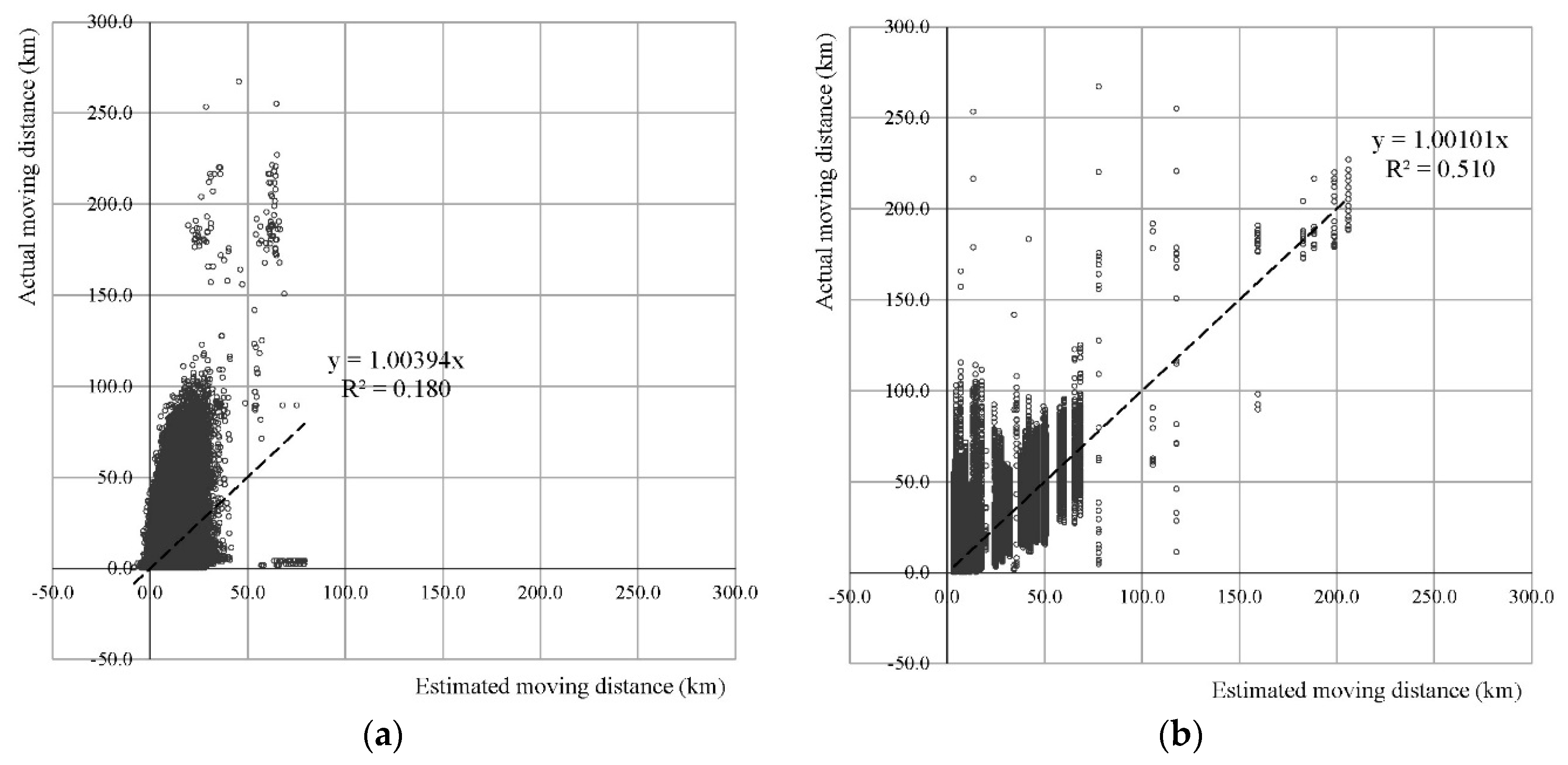
5.1. Comparison of the Empirical Results Between Ordinary Least Squares and Decision Tree Regressions

In this study, the empirical analysis of residential relocation distance in the SMR included the application of ordinary least squares regression and decision tree regression using a machine learning approach. The results of the empirical analysis are summarised in Table 5.
First, the training and test R-squared values in the ordinary least squares regression model were 0.180 and 0.190, respectively, showing low explanatory power. In the household attributes domain, among the residential moving reasons, house was an influencing factor that shortened the moving distance of households by about two kilometres compared to other reasons. This can be interpreted as a result of the existence and influence of the housing sub-market in the SMR. On the other hand, job and education were significant factors—these were significant factors affecting residential mobility in previous studies [7,48]—in increasing the distance of residential movement of households over five km compared to other causes. Age and squared age were significant variables, and the residential relocation distance of households was the lowest at the householder age of approximately 59, which is similar to the residential mobility of the life cycle model.
For the explanatory variables that represent composition of a household, the number of household members and the number of children had negative coefficients at the 99% level. These outcomes are similar to previous results related to mobility based on residential duration [49], which can be understood that households with more members have more complex decision-making systems for their residential relocation and there is a tendency to maintain their community that was formed in the previous location. Notably, sex was a positive determinant at the 99% level. This result can be interpreted as the relatively low resistance to residential moving distance in the households with a male householder or the long-distance residential movements due to changes in the workplace of the male householder.
In the location characteristics domain, the most important explanatory variable was accessibility to employment markets in the both the origin and destination residential locations. Accessibility variables had negative coefficients, which implies the importance of proximity to employment centres affecting residential location choice of household in previous studies [7,50,51,52]. Density and proportion of new buildings within one year or five years also had significant coefficients, but their signs showed opposite values in origin and destination locations of the residential movements. High population density is considered a negative determinant of residential environment [53], whereas newly constructed houses are seen as positive. Since the former and the latter are a push factor and a pull factor [54], respectively, the difference in the distance as well as the migration flow of intra-urban residential mobility can be generated. Housing ownership had negative coefficients in both the origin and destination locations. These results can be interpreted as the relatively short movement of residents living in stabilised settlements based on the high proportion of housing ownership. Moreover, the coefficient of bus availability, which is the number of inter-regional bus routes by administrative district, was significantly positive only in the destination residential location. This outcome means that even though it is located far away, a district with a large number of bus routes with relatively high inter-regional mobility can be an attractive residential moving destination.
Second, in decision trees, the complex tree constructed using the training dataset generally has an overfitting problem. Therefore, by setting the parameters for maximum depth and the leaf node minimum sample value, an early stopping method was applied to terminate the learning algorithm before the tree became too complex [55]. The application of early stopping has the advantages of not only mitigating the overfitting problem, but also interpreting the derived tree structure. A trial and error method was applied to set the appropriate parameter values: the maximum depth was six, and the leaf node minimum sample value was 10 (Appendix A).
In the model applying decision tree regression, the explanatory powers of the final derived model showed a remarkable improvement over the ordinary least squares regression model. The training R2 value was 0.512, and the test value was 0.504. Twelve features were contained in the derived decision tree. The importance of features reflects the contribution each variable makes in estimating the target variable, which is the residential relocation distance of each household in this study. The importance of a feature was estimated as the normalised total reduction of the criterion caused by the feature. In Table 5, two of the most important features were accessibility to employment markets in the locations before and after the residential movement. Among the residential moving reasons, job was ranked as the third most important feature. The importance of these three features accounted for approximately 95% of the total importance. In addition, in terms of importance, the following features are ranked: density of population in destination and origin locations, members, new buildings within five years in origin residential location, moving reason: education, age of householder, bus availability in destination, and housing ownership in destination and origin residential locations. These importance values are different from the standardised beta values that indicate the relative influence of explanatory variables on the results of the ordinary least squares regression model.
Decision trees, while not as powerful from a pure machine learning standpoint, are still one of the canonical examples of an understandable machine learning algorithm. That is, the structure of the derived decision tree can be represented as shown in Figure 3. In the figure, the grey circle indicates a leaf node that is composed of 57 nodes, and intermediate nodes are represented using 56 white circles. Among them, the leftmost white circle is called the root node. In this study, the derived decision tree structure can be traced back to the splits from the training dataset starting with 156,939 samples at the root node. Moreover, in the tree structure, the solid lines mean that an observation goes to the lower branch if the condition shown at the intermediate node is satisfied, whereas the broken lines indicate that an observation proceeds to the upper branch if it is not satisfied. The equations presented on the right side of the intermediate nodes (white circles) are conditions splitting the assigned samples of each node, and X(n) denotes the explanatory variables in Table 5. Of the two numbers located to the right of the leaf nodes (grey circles), the first and second numbers are the number of samples and the average relocation distance of the assigned samples to the nodes, respectively. In addition, Figure 3 shows the many paths based on the decision tree of households related to the residential relocation distance in the SMR. In a decision tree model, describing the entire tree structure is not only extremely complex, but also inefficient. Therefore, the most important top three assigned leaf nodes and their assigned paths are described in this paper. The red solid and broken lines represent branch paths that reach the leaf nodes to which the top three most-allocated samples are assigned.
First, the leaf node with the largest number of samples contains 43,880 households (27.96%) with an average residential moving distance of 6.866 km. The features affecting the path of branches to the leaf node were residential mobility caused by factors other than job or education: X(0) and X(2), higher potential accessibility to employment markets from origin to destination residential location, X(11) and X(18), and one-person household (X(6)). This result can be summarised as the pattern of general residential movements based on the employment market in the one-person household group. Second, the leaf node with the second largest number of samples includes 38,003 households (24.22%), with an average residential relocation distance of 3.312 km, which is the shortest distance leaf node in this derived tree. The features related to the leaf node were residential mobility, caused by factors other than job X(0), higher potential accessibility to employment markets from origin to destination residential location, X(11) and X(18), densely populated origin and destination locations, X(12) and X(19), and households with more than two people, X(6). This path can be understood as the shortest residential moving pattern of households with more than two members based on accessibility to employment markets, which occur among densely populated districts, for purposes other than a job. Finally, the path related to the third largest leaf node includes 9,732 households (6.20%) with an average moving distance of 8.323 km, which was affected by the features including residential mobility caused by job X(0) and lower potential accessibility to employment markets from origin to destination location, X(11) and X(18). This result can be interpreted as the relatively longer residential moving distance of households caused by job or employment except other residential conditions (Figure 4 and Appendix B).

5.2. Application of Ordinary Least Squares Regression and Decision Tree Regression Models

This study focuses not only on the identification of the features and their structures affecting residential relocation distance but also on the applicability of the machine learning approach to residential mobile pattern analysis. Therefore, the application results of the previously constructed regression models and the actual moving distance values were directly compared.
Figure 5 compares the application results. The figure on the left is the result of comparing the actual moving distances of all samples and the estimated moving distance using the ordinary least squares regression model. The figure on the right is the comparison of the actual distance and the estimated distance using the decision tree regression model. As expected, the decision tree regression model results were relatively better. The application of the ordinary least squares regression model showed a large number of underestimated values and a large number of unrealistic residential moving distances, such as values less than zero, whereas the results of the decision tree application presented relatively few underestimated values, and there were no unrealistic estimates of the residential relocation distance. Thus, in the latter, the regression coefficient (1.00101) and the R2 value (0.510) were also better.

6. Summary and Concluding Remarks

In the rapidly changing Korean housing market, from both the supply and demand perspectives, understanding the spatial patterns of residential relocation is a meaningful goal. This paper focused on the structure among determinants affecting residential relocation distance and the applicability of a new approach using spatial Big Data and machine learning methodology. To this end, the available microdata on household residential movement was converted into spatial Big Data, and spatial Big Data and the decision tree regression model were applied in an empirical study. The results of the empirical analysis on residential relocation distance in the SMR using ordinary least squares and decision tree regressions can be summarised as follows.
In terms of explanatory power, the decision tree regression model showed better performance than the ordinary least squares regression model. Twenty variables were significant in the ordinary least squares regression, whereas only 12 features were applied in the decision tree regression model, although the model had a relatively complicated structure. As a result of the ordinary least squares regression, residential movements for housing-related reasons were shorter than the distance of residential movements caused by job or education. Households with a householder over 60 years old or male householders had longer residential relocation distances. On the other hand, households with a householder less than 60 years old, households with multiple members, and households with school-aged children moved to a relatively close residential district. In terms of the location characteristics in the origin and destination, accessibility to employment markets and housing ownership were the factors that shortened the household residential relocation distance. In the origin, the high population density led to longer residential movements, and the variables associated with the proportion of new buildings were factors that shortened the residential moving distance. However, those in the destination had an opposite effect.
To summarise the main outcomes of the decision tree regression, the most important features that determined the residential relocation distance were migration caused by a job and accessibility to employment markets, although a large number of residential relocations occurred for reasons other than a job. Additionally, this empirical study showed considerable residential movement to the districts with good access to employment. The shortest moving distance was found when households with more than two people moved among densely-populated districts, whereas residential movements caused by a job had a relatively longer moving distance.
Moreover, the ordinary least squares regression and the decision tree regression models were applied to compare their estimated values and the actual measurements based on the geographic data using the Internal Migration Statistics microdata. The estimated distances using the decision tree regression model were more realistic, with the estimated moving distances not containing values less than zero with few underestimated values. Its explanatory power was higher than that of the ordinary least squares regression model.
Thus, this study reviewed the applicability of the machine learning method using spatial Big Data, which is a focus in the field of urban planning and management. In particular, this article attempted to overcome the limitation of conventional statistical models—low explanatory power and a lot of rigid constraints—using an interpretable and understandable machine learning model: the decision tree regression model. The results of this study have the following implications. First, the result of the decision tree regression model (training R2: 0.512) showed a significant improvement in the explanatory power compared to that of the ordinary least squares regression model (training R2: 0.180), which is similar to a conventional linear regression model. Second, the derived decision tree presented not only the diversity of structures that determine the residential relocation distance, but also the main features, such as movement caused by jobs and accessibility to employment markets, which form the structure. Finally, for the residential moving pattern, we found that the machine learning approach, including decision trees, can estimate more realistic results than conventional methodologies.
The development of the forecasting model beyond the empirical analysis of the decision structures for the residential relocation distance, and the inclusion of several explanatory variables that were not contained in the model, require further research. For instance, explanatory variables that can be derived from data including spatial information could be applied to the machine learning approach via that information. In addition, the inclusion of qualitative information, such as individual movement trajectories and individual preferences, into the machine learning approach is also a future research topic. Despite of these future tasks, this study presented a case using the machine learning approach with spatial Big Data in the urban planning and management field. Moreover, the outcomes of this research provide significant information about the sustainable urban management of metropolitan residential districts and the construction of reasonable housing policies in terms of the public debate of housing and residential location issues. Additionally, this study Is expected to be the basis of further studies of spatial patterns of residential relocation in the future, because this study could be a starting point for using new innovative approaches, such as the machine learning method.

Author Contributions

Conceptualization, C.Y.; Formal analysis, K.K.; Investigation, C.Y.; Methodology, C.Y. and K.K.; Supervision, C.Y.; Validation, K.K.; Visualization, C.Y.; Writing—original draft, C.Y.; Writing—review & editing, C.Y.

Funding

This research was supported by Basic Science Research Program through the National Research Foundation of Korea (NRF) funded by the Ministry of Education (2016R1D1A1B03930624).

Conflicts of Interest

The authors declare no conflict of interest. The founding sponsors had no role in the design of the study; in the collection, analyses, or interpretation of data; in the writing of the manuscript, and in the decision to publish the results.

Appendix A

Regarding the selection of the appropriate parameters of the decision tree for controlling the overfitting problem, a trial and error method was applied in this study. In Figure A1, the figure on the left represents the variation of the mean squared error value (MSE) according to the leaf node minimum sample value. The variation in the MSEs according to the leaf node minimum sample value without setting the depth of the tree shows the lowest level from 9 to 12 samples. The figure on the right indicates the variation of the R-squared values according to depth of tree after the leaf node minimum sample value is set to 10. The R-squared values, which mean the explanatory powers of the models applied to the training dataset and the test dataset, show the gaps of less than 1% up to a depth of 6. Therefore, the appropriate parameter values of this decision tree regression model were selected as follows: the leaf node’s minimum sample value is 10 and the maximum depth is 6.
Figure A1. (a) Variation of the mean squared errors according to the leaf node minimum sample value; (b) Variation of the R-squared values according to depth of tree.
Sustainability 10 02996 g0a1

Appendix B

As shown in the following figures, the spatial distribution of departing and arriving households’ shares by area is generally similar, but the share of arriving households is somewhat higher in the outside areas of Seoul than the share of departing households in the SMR. In addition, the areas with high shares in specific regions form a cluster, which are generally close to employment centres.
Figure A2. (a) Share of departing households by area; (b) Share of arriving households by area.
Sustainability 10 02996 g0a2

References

  1. Seo, D.; Kwon, Y. In-migration and housing choice in Ho Chi Minh City: Toward sustainable housing development in Vietnam. Sustainability 2017, 9, 1738. [Google Scholar] [CrossRef]
  2. Rossi, P.H. Why Families Move: A Study in The Social Psychology of Urban Residential Mobility; Free Press: New York, NY, USA, 1955. [Google Scholar]
  3. Hoyt, H. The Structure and Growth of Residential Neighborhoods in American Cities; U.S. Government Printing Office: Washington, DC, USA, 1939.
  4. Ravenstein, E.G. The Laws of Migration. J. Stat. Soc. Lond. 1885, 48, 167–235. [Google Scholar] [CrossRef]
  5. Park, E.; Lee, J.W. A study on policy literacy and public attitudes toward government innovation-focusing on Government 3.0 in South Korea. J. Open Innov. Technol. Mark. Complex. 2015, 1, 1–13. [Google Scholar] [CrossRef]
  6. Nho, H.J. Research ethics education in Korea for overcoming culture and value system differences. J. Open Innov. Technol. Mark. Complex. 2016, 2, 1–11. [Google Scholar] [CrossRef]
  7. Yi, C.; Lee, S. An empirical analysis of the characteristics of residential location choice in the rapidly changing Korean housing market. Cities 2014, 39, 156–163. [Google Scholar] [CrossRef]
  8. OECD. OECD Regions at a Glance 2016; OECD Publishing: Paris, France, 2016; ISBN 9789264252097. [Google Scholar]
  9. Kwon, W.Y. An examination of residential location behavior in the Seoul metropolitan area. Ann. Reg. Sci. 1984, 18, 33–48. [Google Scholar] [CrossRef]
  10. The Seoul Institute. Seoul Statistical Series Section 04. Housing; The Seoul Institute: Seoul, Korea, 2014.
  11. Hong, S.; Lee, Y. Limitation of residential mobility distance in seoul metropolitan area -focused on migration region and family size-. Korea Real Estate Acad. Rev. 2015, 60, 115–126. [Google Scholar]
  12. Brown, L.A.; Moore, E.G. The inter-urban migration process: A perspective. Geogr. Ann. Ser. B Hum. Geogr. 1970, 52, 1–13. [Google Scholar] [CrossRef]
  13. Chun, H.S. The characteristics of housing mobility of the residents’ in new town areas. Gyeonggi Forum 2004, 6, 91–111. [Google Scholar]
  14. Wu, F. Intraurban residential relocation in Shanghai: Modes and stratification. Environ. Plan. A 2004, 36, 7–25. [Google Scholar] [CrossRef]
  15. Moore, E.G. Residential Mobility in The City; Association of American Geographers: Washington, DC, USA, 1972. [Google Scholar]
  16. Loren, D.L.; Eva, K.; Boaz, K. Residential relocation of amenity migrants to Florida: “Unpacking” post-amenity moves. J. Aging Health 2010, 22, 1001–1028. [Google Scholar] [CrossRef]
  17. Lee, B.H.Y.; Paul, W. Residential mobility and location choice: A nested logit model with sampling of alternatives. Transportation (Amst.) 2010, 37, 587–601. [Google Scholar] [CrossRef]
  18. Stapleton, C.M. Reformulation of the family life-cycle concept: Implications for residential mobility. Environ. Plan. A 1980, 12, 1103–1118. [Google Scholar] [CrossRef]
  19. Pickvance, C.G. Life cycle, housing tenure and residential mobility: A path analytic approach. Urban Stud. 1974, 11, 171–188. [Google Scholar] [CrossRef]
  20. Morris, E.W.; Crull, S.R.; Winter, M. Housing Norms, housing satisfaction and the propensity to move. J. Marriage Fam. 1976, 38, 309–320. [Google Scholar] [CrossRef]
  21. Chevan, A. Family growth, household density, and moving. Demography 1971, 8, 451–458. [Google Scholar] [CrossRef] [PubMed]
  22. Eluru, N.; Sener, I.N.; Bhat, C.R.; Pendyala, R.M.; Axhausen, K.W. Understanding residential mobility: joint model of the reason for residential relocation and stay duration. Transp. Res. Rec. 2009, 2133, 64–74. [Google Scholar] [CrossRef]
  23. Zanganeh, Y.; Hamidian, A.; Karimi, H. The analysis of factors affecting the residential mobility of afghan immigrants residing in mashhad (case study: Municipality regions 4, 5 and 6). Asian Soc. Sci. 2016, 12, 61–69. [Google Scholar] [CrossRef]
  24. Ha, S.K. Housing Policy and Practice in Korea, 3rd ed.; Pakyoungsa: Seoul, Korea, 2006. [Google Scholar]
  25. Min, B.; Byun, M. Residential mobility of the population of seoul: Spatial analysis and the classification of residential mobiltiy. Seoul Stud. 2017, 18, 850102. [Google Scholar]
  26. Clark, W.A.V.; Onaka, J.L. Life cycle and housing adjustment as explanations of residential mobility. Urban Stud. 1983, 20, 47–57. [Google Scholar] [CrossRef]
  27. Yi, C.; Lee, S. Analyzing the factors on residential mobility according to the household member’s change—In consideration of residential duration of the households in the Seoul metropolitan area. J. Korea Plan. Assoc. 2012, 47, 205–217. [Google Scholar]
  28. Yee, W.; van Arsdol, M.D.J. Residential mobility, age, and the life cycle. J. Gerontol. 1977, 32, 211–221. [Google Scholar] [CrossRef]
  29. Clark, W.A.V. Life course events and residential change: Unpacking age effects on the probability of moving. J. Popul. Res. 2013, 30, 319–334. [Google Scholar] [CrossRef]
  30. Burnley, I.H.; Murphy, P.A.; Jenner, A. Selecting suburbia: Residential relocation to outer Sydney. Urban Stud. 1997, 34, 1109–1127. [Google Scholar] [CrossRef]
  31. Yang, J. Transportation implications of land development in a transitional economy: Evidence from housing relocation in Beijing. Transp. Res. Rec. 1996, 1954, 7–14. [Google Scholar] [CrossRef]
  32. Clark, W.A.V.; Dieleman, F.M. Households and Housing: Choice and Outcomes in The Housing Market; Center for Urban Policy Research: New Brunswick, NJ, USA, 1996; ISBN 9780882851563. [Google Scholar]
  33. Dieleman, F.M. Modelling residential mobility: A review of recent trends in research. J. Hous. Built Environ. 2001, 16, 249–265. [Google Scholar] [CrossRef]
  34. Niedomysl, T. How migration motives change over migration distance: Evidence on variation across socio-economic and demographic groups. Reg. Stud. 2011, 45, 843–855. [Google Scholar] [CrossRef]
  35. Niedomysl, T.; Fransson, U. On distance and the spatial dimension in the definition of internal migration. Ann. Assoc. Am. Geogr. 2014, 104, 357–372. [Google Scholar] [CrossRef]
  36. Niedomysl, T.; Ernstson, U.; Fransson, U. The accuracy of migration distance measures. Popul. Space Place 2017, 23. [Google Scholar] [CrossRef]
  37. Shalev-Shwartz, S.; Ben-david, S. Understanding Machine Learning: From Theory to Algorithms, 1st ed.; Cambridge University Press: New York, NY, USA, 2014; ISBN 9781107057135. [Google Scholar]
  38. Witten, I.H.; Frank, E. Data Mining: Practical Machine Learning Tools and Techniques, 2nd ed.; Morgan Kaufmann: San Francisco, CA, USA, 2005; ISBN 0120884070. [Google Scholar]
  39. Zhang, H.; Wu, P.; Yin, A.; Yang, X.; Zhang, M.; Gao, C. Prediction of soil organic carbon in an intensively managed reclamation zone of eastern China: A comparison of multiple linear regressions and the random forest model. Sci. Total Environ. 2017, 592, 704–713. [Google Scholar] [CrossRef] [PubMed]
  40. Estelles-lopez, L.; Ropodi, A.; Pavlidis, D.; Fotopoulou, J.; Gkousari, C.; Peyrodie, A.; Panagou, E.; Nychas, G.J.; Mohareb, F. An automated ranking platform for machine learning regression models for meat spoilage prediction using multi-spectral imaging and metabolic profiling. Food Res. Int. 2017, 99, 206–215. [Google Scholar] [CrossRef] [PubMed]
  41. Chagas, C.; Junior, W.; Bhering, S.; Filho, B. Spatial prediction of soil surface texture in a semiarid region using random forest and multiple linear regressions. Catena 2016, 139, 232–240. [Google Scholar] [CrossRef]
  42. Oliveira, M.; Gama, J. An overview of social network analysis. WIREs Data Min. Knowl. Discov. 2012, 2, 99–105. [Google Scholar] [CrossRef]
  43. Tso, G.K.F.; Yau, K.K.W. Predicting electricity energy consumption: A comparison of regression analysis, decision tree and neural networks. Energy 2007, 32, 1761–1768. [Google Scholar] [CrossRef]
  44. Xu, M.; Watanachaturaporn, P.; Varshney, P.K.; Arora, M.K. Decision tree regression for soft classification of remote sensing data. Remote Sens. Environ. 2005, 97, 322–336. [Google Scholar] [CrossRef]
  45. Prasad, A.M.; Iverson, L.R.; Liaw, A. Newer classification and regression tree techniques: bagging and random forests for ecological prediction. Ecosystems 2006, 9, 181–199. [Google Scholar] [CrossRef]
  46. Hansen, W.G. How accessibility shapes land use. J. Am. Inst. Plann. 1959, 25, 73–76. [Google Scholar] [CrossRef]
  47. Wilson, A.G. Entropy in Urban and Regional Modeling; Pion: London, UK, 1970. [Google Scholar]
  48. Yi, Y.; Kim, E.; Choi, E. Linkage among school performance, housing prices, and residential mobility. Sustainability 2017, 9, 1075. [Google Scholar] [CrossRef]
  49. Choi, Y.; Yim, H.K. Determinants of the Residents’ Settlements Employing Poission Regression. Korea Spat. Plan. Rev. 2005, 46, 99–114. [Google Scholar]
  50. Pagliara, F.; Simmonds, D. Conclusions. In Residential Location Choice-Models and Applications; Pagliara, F., Preston, J., Simmonds, D., Eds.; Springer: Berlin, Germany, 2010; pp. 243–248. [Google Scholar]
  51. Simmonds, D. The DELTA residential location model. In Residential Location Choice-Models and Applications; Pagliara, F., Preston, J., Simmonds, D., Eds.; Springer: Berlin, Germany, 2010; pp. 77–97. [Google Scholar]
  52. Waddell, P. Modelling residential location in UrbanSim. In Residential Location Choice-Models and Applications; Pagliara, F., Preston, J., Simmonds, D., Eds.; Springer: Berlin, Germany, 2010; pp. 165–180. [Google Scholar]
  53. Cadwallader, M. Migration and Residential Mobility: Macro and Micro Approaches; University of Wisconsin Press: Madision, WI, USA, 1992. [Google Scholar]
  54. Cluttons. Residential Mobility in London: Unlocking Migration Patterns; Cluttons LLP: London, UK, 2017. [Google Scholar]
  55. Mueller, A.C.; Guido, S. Introduction to Machine Learning With Python; O’Reilly: Sebastopol, CA, USA, 2016; ISBN 9781491917213. [Google Scholar]
Figure 1. (a) Location of the Seoul metropolitan region (SMR) in Korea; (b) Components of SMR.
Sustainability 10 02996 g001
Figure 2. Relocation distance based on (a) family size and (b) age group of householder.
Sustainability 10 02996 g002
Figure 3. Decision tree for residential relocation distance of the households in SMR.
Sustainability 10 02996 g003
Figure 4. Detailed branch paths to the leaf nodes with the top three largest number of samples.
Sustainability 10 02996 g004
Figure 5. Result of applying the (a) ordinary least squares regression model and (b) tree regression model.
Sustainability 10 02996 g005
Table 1. Seoul metropolitan region (SMR) characteristics.
ItemTotalSeoulIncheonGyeonggi
Population (million people)23.9069.3952.76711.744
Household (million households)9.5193.9151.0664.538
Area (km2)11,828605104810,175
City, county and borough levelSi28--28
Gun5-23
Gu5325820
Minimum-sized administrative area levelEup34-133
Myeon127-19108
Dong972424129419
Source: Statistics of Urban Planning in 2015, 2015 Census in Korea.
Table 2. Frequency and distance of residential movements.
ItemSMRSeoulIncheonGyeonggi
Frequency of residential movementsTotal3,107,134
(100.0%)
1,287,379
(100.0%)
352,488
(100.0%)
1,467,267
(100.0%)
Inside2,747,380
(88.4%)
882,299
(68.5%)
247,760
(70.3%)
1,081,897
(73.7%)
Outside359,754
(11.6%)
405,080
(31.5%)
104,728
(29.7%)
385,370
(26.3%)
Movement per household0.3260.3290.3310.323
Residential relocation distance 1 (km)Total9.1237.7538.89410.391
Inside-3.9404.3047.965
Outside-23.90929.11225.412
1 The average Euclidian distance calculated using 10% randomly sampled data from the raw data.
Table 3. Explanatory variables applied in the empirical analysis.
VariableDescriptionUnitSource
Household attributesMoving reasonMajor reasons for residential relocation: job, house, education-The microdata of Internal Migration Statistics
AgeAge of householderYear
SexMale and female-
MembersNumber of household membersPeople
Elderly peopleNumber of elderly household membersPeople
ChildrenNumber of school-aged children: primary, secondaryPeople
Proportion of menProportion of male household members%
Location characteristics 1AccessibilityAccessibility to employment market-Census on Establishments
DensityPopulation densityPeople/haPopulation Census
New buildingProportion of new building;
1 year/5 years
%Housing Census
Housing ownershipRatio of owner-occupied housing%Population Census
Rail availabilityRatio of rail catchment area%Korea Transport Database
Bus availabilityNumber of metropolitan bus routesEA
1 The variables contained in the domain of location characteristics were calculated for both origin and destination locations.
Table 4. Descriptive statistics.
VariableUnitAverageSDMinimumMaximum
-Relocation distancekm9.1213.660.24267.31
Household attributesMoving reason: Job 1-0.190.390.001.00
Moving reason: House 1-0.600.490.001.00
Moving reason: Education 1-0.020.140.001.00
AgeYears44.3213.790.00103.00
Sex: Male 1-0.660.470.001.00
MembersPeople2.101.301.009.00
Elderly peoplePeople0.140.410.004.00
Children: PrimaryPeople0.120.400.004.00
Children: SecondaryPeople0.140.420.007.00
Proportion of men%53.5238.270.00100.00
Location characteristics in originAccessibility-14.260.536.4014.79
DensityPeople/ha174.25129.140.00550.00
New building: 1 year%2.932.460.2717.36
New building: 5 years%13.696.121.8334.89
Housing ownership%48.558.4529.3879.26
Rail availability%25.3927.760.00100.00
Bus availabilityEA7.5410.110.0071.00
Location characteristics in destinationAccessibility-14.230.546.4014.79
DensityPeople/ha167.34129.290.00550.00
New building: 1 year%3.112.740.2717.36
New building: 5 years%14.046.261.8334.89
Housing ownership%48.818.3929.3879.26
Rail availability%24.4627.580.00100.00
Bus availabilityEA7.6610.280.0071.00
1 A reference of nominal variables.
Table 5. Results of the empirical analysis using machine learning models.
Variable (Feature)Ordinary Least Squares RegressionDecision Tree Regression
βStd. βSig.ImportanceRank
(Constant)136.3587 0.000**
Household attributesX(0)Moving reason: Job5.68362.24010.000**0.131803
X(1)Moving reason: House–1.9648–0.96300.000**--
X(2)Moving reason: Education5.48270.76880.000**0.002898
X(3)Age–0.2362–3.26020.000**0.001149
X(4)Squared Age0.00202.78130.000**--
X(5)Sex: Male0.59350.28090.000**--
X(6)Members–1.0025–1.30520.000**0.012466
X(7)Elderly people0.16310.06680.140 --
X(8)Children: Primary–0.5795–0.23380.000**--
X(9)Children: Secondary–0.8717–0.36970.000**--
X(10)Proportion of men0.00190.07390.154 --
Location characteristics in originX(11)Accessibility–2.0368–1.07660.000**0.579761
X(12)Density0.00080.10810.015*0.014505
X(13)New building: 1 year–0.1787–0.44110.000**--
X(14)New building: 5 years–0.0461–0.28240.000**0.004347
X(15)Housing ownership–0.0417–0.35230.000**0.0000112
X(16)Rail availability0.00140.03920.352 --
X(17)Bus availability0.00550.05530.138 --
Location characteristics in destinationX(18)Accessibility–6.1138–3.29530.000**0.234332
X(19)Density–0.0026–0.33580.000**0.017494
X(20)New building: 1 year0.11470.31560.000**--
X(21)New building: 5 years0.04340.27190.000**--
X(22)Housing ownership–0.0271–0.22770.000**0.0003911
X(23)Rail availability0.00190.05260.219 --
X(24)Bus availability0.04340.44570.000**0.0009010
Explanatory PowerTraining R2: 0.180
Test R2: 0.190
Training R2: 0.512
Test R2: 0.504
* p-value < 0.05; ** p-value < 0.01.

