Short-Term Forecasting of Land Use Change Using Recurrent Neural Network Models


1
Spatial Analysis and Modeling Laboratory, Department of Geography, Simon Fraser University, University Drive, Burnaby, BC V5A1S6, Canada
2
GIS and GeoCollaboration Laboratory, Department of Civil Engineering, Ryerson University, 350 Victoria Street, Toronto, ON M5B 2K3, Canada
*
Authors to whom correspondence should be addressed.
Sustainability 2019, 11(19), 5376; https://doi.org/10.3390/su11195376
Submission received: 12 July 2019
/
Revised: 17 September 2019
/
Accepted: 24 September 2019
/
Published: 28 September 2019
(This article belongs to the Special Issue Applications of Artificial Intelligence in the Study of Land Use and Land Cover Change)
Abstract
:Land use change (LUC) is a dynamic process that significantly affects the environment, and various approaches have been proposed to analyze and model LUC for sustainable land use management and decision making. Recurrent neural network (RNN) models are part of deep learning (DL) approaches, which have the capability to capture spatial and temporal features from time-series data and sequential data. The main objective of this study was to examine variants of the RNN models by applying and comparing them when forecasting LUC in short time periods. Historical land use data for the City of Surrey, British Columbia, Canada were used to implement the several variants of the RNN models. The land use (LU) data for years 1996, 2001, 2006, and 2011 were used to train the DL models to enable the short-term forecast for the year 2016. For the 2011 to 2016 period, only 4.5% of the land use in the study area had changed. The results indicate that an overall accuracy of 86.9% was achieved, while actual changes in each LU type were forecasted with a relatively lower accuracy. However, only 25% of changed raster cells correctly forecasted the land use change. This research study demonstrates that RNN models provide a suite of valuable tools for short-term LUC forecast that can inform and complement the traditional long-term planning process; however, further additional geospatial data layers and considerations of driving factors of LUC need to be incorporated for model improvements.
1. Introduction
Land use change (LUC) arises from human-environmental interactions [1], and so far, about 39% of the Earth’s land has never been exploited or used for the benefits of humans [2]. Land use change (LUC) with urban intensification has resulted in pressures to the natural environment that can produce irreversible damages, if not adequately addressed. Better knowledge and understanding of LUC process can help policymakers to make informed decisions for sustainable land management. Sustainable land management practices promote the activities that increase the benefit of utilization and development of land resources for individual, social, and economic purposes. LUC analysis and modeling methods can assist in the projection of possible future LU patterns, thus helping and guiding the management of land towards sustainable urban development.
The LUC phenomenon is typically studied through earth observations (EO), remote sensing (RS), and field measurements [3], all of which provide the opportunity for monitoring and quantifying changes of LU patterns at local, regional, and global levels. LUC is a complex phenomenon occurring locally and with implications for global geographic scales. Decades ago, RS sensors provided data with lower resolution, and the availability of this data to the public was very limited. Besides EO and RS techniques that require advanced satellite equipment and expert knowledge for data interpretation, researchers have been using LUC modeling approaches for decades. LUC models provide representations and strategies that can help analyze, understand and assist in the planning and management of land and natural resources. Many LUC models are based on inductive approaches which start with studying the observations and then developing explanations [4,5]. LUC models are often based on a suite of explanatory variables that potentially drive the change process. However, the main factors of LUC are directly related to human interactions and decision-making processes that are often difficult to accurately model and predict.
Deep learning (DL) is a subset of machine learning (ML) approaches and can be considered as deep machine learning. ML and DL both work by reducing the dimensionality and extracting features of large datasets. Compared with traditional ML methods, DL models can simultaneously extract and classify features with faster computation. Recent access to larger volumes of data from open sources coupled with superior computational abilities has given DL models great potential to become valuable tools that are capable of exploring and analyzing LUC phenomena. DL models include both convolutional neural networks (CNN) [6] and recurrent neural networks (RNN) [7]. CNNs have been used for image classification [8] and LUC classification and mapping [9], while RNNs have been used for natural language processing (NLP) tasks [10,11]. Deep learning (DL) has been identified as an intelligent modeling approach for advancing the field of LU modeling [12,13].
RNNs have the capability to capture information within sequential datasets such as in spatial and temporal sequences [14]. Due to the spatio-temporal nature of LUC processes, the main objective of this research study is to examine the capabilities of RNN-based models to model LUC from an integrated space-time perspective and to perform short-term forecast of LU. Sequential land use data for the City of Surrey, British Columbia, Canada were used to implement the selected RNN models and generate the forecasted LUC.
1.1. Land Use Change Models
The usual approaches for monitoring urban growth and LUC detection are based on geographic information systems (GIS) and RS [15] techniques and available geospatial datasets, which may require intensive pre-processing and interpretation. Efforts have been made to model LUC with the projection of possible future scenarios for spatial patterns of change to provide solutions and assistance to land management. In the published research literature, various LUC modeling methods have been reported such as Markov chains [16,17], cellular automata [18,19,20,21,22], neural networks [23,24,25], logistic regression [26], multi-agent systems [27,28], and machine learning [29,30,31,32].
Markov chains is a stochastic model that can capture time dependency among sequential data and is usually used to describe a sequence of possible events or states whose probabilities only depend on previous events or states. Markov chains cannot preserve the information from the event that is not within the neighborhood of a current event. There are some Markov chain-based models for representing the dynamics of LU systems [17], which project the future LU by applying a transition probability matrix on the primary matrix recording LU information. Markov chains model assume that the transition probability between each pair of states is stationary over time; hence, these models can forecast LUC from short to long-term. However, Markov chain models cannot consider socioeconomic and human related factors that can potentially lead to changes in LU patterns.
Cellular automata (CA) is a discrete modeling approach that has been used for representing LUC given its capability to capture both spatial and temporal dynamics of a phenomenon and consider changes at a very local scale [33,34,35]. The CA consists of a regular grid of cells, where each cell has one of many finite states, and the state of a cell changes in the next time iteration according to the function of transition rules based on the state of the cell and in its spatial neighborhood. The structure of CA models has a close affinity with raster-based GIS and RS datasets. However, Stevens and Dragićević [36] proposed a LUC model using irregular CA cells, although this requires longer computation time. The integration of Markov chains and CA allows for the simulation of spatial and temporal LUC processes [37]. Even though the fixed rules enable the various possibilities of transition, the forecast of LUC is more precise when the system is stable over years and under the assumptions that the land always changes with the same transition rules. The assumption of an ideal and stable environment is not realistic as LU changes are governed by human decisions changing over time that are difficult to predict. However, these types of models are more sensitive to spatial than temporal factors.
Machine learning (ML) methods depend on strong statistical learning theory where the size and quality of the training datasets significantly influence the performance of ML methods. ML-based LUC models can extract and learn from earlier LU observations the driving forces of LUC and their impact. Otukei and Blaschke [31] evaluated several ML methods, such as artificial neural networks (ANN), support vector machine (SVM), maximum likelihood, and decision trees, to investigate LUC detection, and their study demonstrated better classification performance of SVM and ANN algorithms. Samardzic-Petrovic et al. [38] compared the performance of some common ML methods for LUC short-term forecasting. Urban LUC was also modeled using decision trees [39] and SVM [32]. However, traditional ML methods have limited performance, when the data is highly dimensional and the number of observations is large [40].
Post-classification comparison is the strategy of some ML-based LUC detection methods. The change analysis of multi-temporal images generally employs two basic methods: raster-to-raster comparison and post-classification comparison [41]. Other ML methods assume the independence of data [42]; however, spatial data are often known for their dependency and spatial autocorrelations. Therefore, using DL models compared to ML brings the advantage of automating the extraction of representations (abstractions) from a larger amount of data. The success of DL models has started to attract attention for studies of LUC classification using RS datasets with CNNs.
Recently, some studies have shown the effectiveness of RNN for analyzing LUC. Byeon et al. [43] conducted LU scene classification with Long Short Term Memory (LSTM) networks instead of CNN without pre-processing, the results of which were comparable to that of CNNs. This study indicates that LSTM models can learn the spatial neighboring context information for every raster and capture the global dataset dependency through the recurrent connections. Using sequence-to-sequence processing of LSTM models, [44] classified land cover through learning from multi-temporal land cover RS datasets. CNN, RNN and LSTM models were used to model vegetation from temporal RS data, and LSTM outperformed CNN as temporal information was used in training [45]. Due to the realistic dynamics of fast-developing urban areas, it is necessary to propose models that are more efficient to capture the change and study the LUC from a spatio-temporal perspective. Bengio [46] used CNN and RNN for learning long-term dependencies and functions from complex phenomenon. RNN models can consider larger numbers of data layers and thus be more effective than traditional ML methods such as SVM or decision tree (DT), to name a few. So far, RNN has recently been used for land cover classification [47,48,49] and land cover change detection [50,51]. Du et al. [52] used RNNs for spatio-temporal modeling of LUC and the overall accuracy results were close to 50%. Therefore, there is a need to further explore the potential of RNNs to forecast LUC. In this research study, previous geospatial LU datasets with 5-year intervals for the City of Surrey, British Columbia, Canada were used to implement the concepts for RNN-based short-term forecasting of LUC.
1.2. RNN and its Variants
Artificial neural networks (ANN) are the collections of connected neurons (also called layers) inspired by the human brain [53]. CNN and RNN are types of ANN. Unlike CNN, which contains different types of layers that perform different functions (e.g., convolutional, pooling and nonlinear layers), the basic RNN consists only of recurrent layers. Each layer in an RNN shares the same group of functions and parameters, while the parameters are updated in each layer. As shown in Figure 1, the connections between recurrent layers are cyclical when presented compactly [54], and for the convenience of visualization, it can be unfolded like a chain-like structure.
CNNs are often used for image classification tasks. The inputs and outputs of CNNs have fixed sizes and are processed independently from each other. By contrast, RNNs can deal with sequential inputs and have sequential outputs, while the inputs are considered dependent so that RNNs can capture their dependence. In reality, many datasets such as text, speech, audio, video, weather, and stock price are sequential and internally dependent. Some applications areas of RNN and its variants include for example music composition [55], handwriting recognition [56], speech synthesis [57], and video captioning [58], to name a few. LSTMs are often used for time-series problems such as predicting stock market price movement [59], weather [60], traffic flow [61], and passenger flow [62].
The traditional RNN has the limitation of short-term memory caused by a vanishing gradient problem [63]. Gradients are used to update the weights of networks, which shrink through time during backpropagation process and may become too small to contribute new significant weights based on Equation (1):
New weights = old weights − (learning rate × gradients).
The problem of short-term memory of traditional RNNs can be solved by long-short term memory (LSTM) [64]. LSTM is one of the variants of RNN, which has unique internal mechanisms called gates that can regulate the flow of information compared with traditional RNN. The function of gates is to decide if the data in a sequence is important or not, then to keep or discard the information from that data. Through gates, the essential information can be preserved even if the sequential data is long. Gated recurrent unit (GRU), another variant of RNN, was first introduced by Cho [65]. GRUs have fewer gates and relatively shorter memory but have faster training processes than LSTMs. GRU has comparable performance to LSTM for music and speech modeling tasks [66]. Bidirectional LSTM (BiLSTM) [67] processes two sequential inputs with the opposite direction so that a current BiLSTM layer has two hidden states which accept past information and future information. Furthermore, the algorithms within BiLSTM layers are the same as that of unidirectional LSTM. BiLSTM is adapted with more complicated situations such as speech [68] and phoneme recognition [69], where the current inputs are influenced by previous and future inputs.
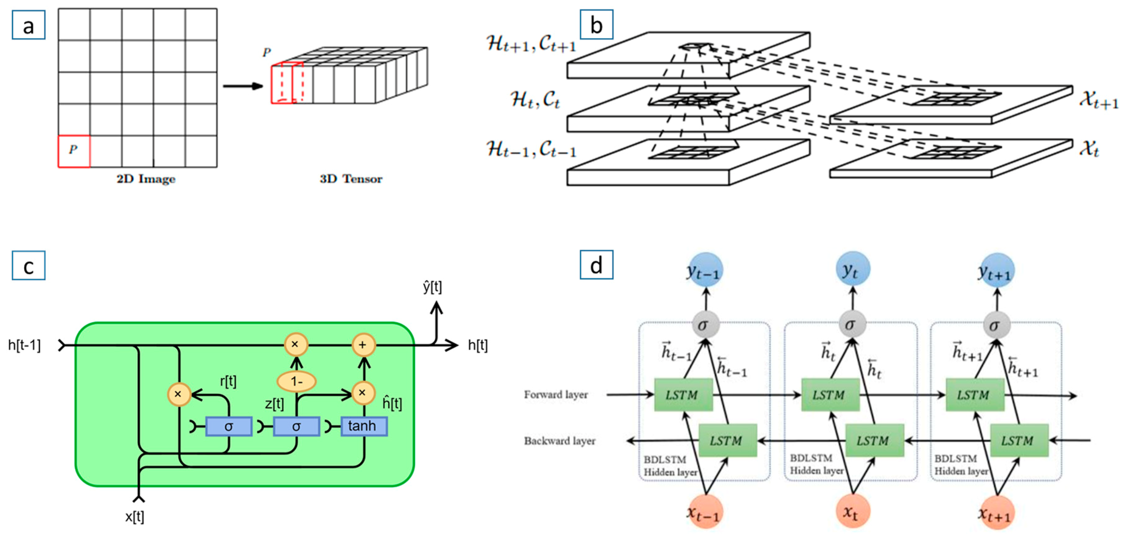
The inputs to RNNs like LSTM and GRU are one-dimensional vectors, while a convolutional LSTM (ConvLSTM) network receives inputs as 3D vectors, which can encode both spatial and temporal information. ConvLSTM is an effective model for nowcasting short-term precipitation within a study area [70]. There also are ConvLSTM based models for short-term forecast of traffic accidents [71], video anomaly detection [72], and short-term forecast of traffic flow [73], and these phenomena have spatial patterns that can be captured by convolutional layers. When using LSTM, it is assumed that each cell is independent. Figure 2a,b present the structure of a ConvLSTM as a group of cells that are located in the same neighborhood. ConvLSTM can simultaneously incorporate the spatial neighborhood for each raster cell and the temporal LU information. The GRU model is very similar to LSTM, however, the difference of GRU is in the update gate and reset gate, where the update gate learns and decides how much of the past information to pass to the future and the reset gate decides how much of the past information to forget (Figure 2c). BiLSTM (Figure 2d) can be considered to have the inputs with the original order and reversed order respectively to feed into the LSTM. RNNs and LSTMs can receive complex sequential inputs or form a hybrid model with other layers or networks [74,75,76].
1.3. LSTM Algorithms
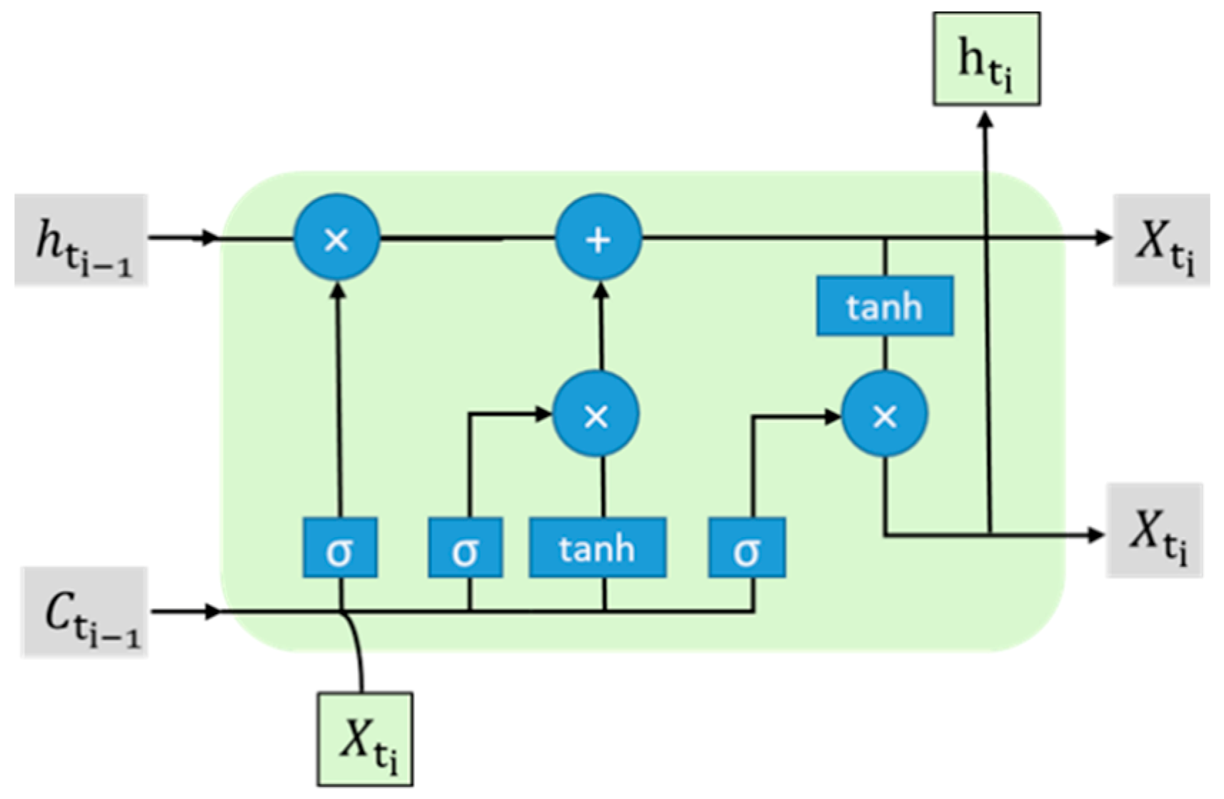
LSTM is more frequently used than traditional RNN due to its longer memory capabilities. The key elements of LSTMs are the cell state, sigmoid activation, forget gate, input gate, and output gate and tanh activation (Figure 3), which control the relevant information through the network. At each processing step, the gates regulate the addition and removal of information to the cell state. Gates have sigmoid activation, which multiplies values between 0 and 1 to derive the percentage of data that will be kept or removed. If the input multiplies with 0, the information is forgotten; if the input multiplies with “1”, the information is remembered. Tanh activation delivers values between −1 and 1. Hochreiter and Schmidhuber [64] provided the Equations (2)–(7) to describe the algorithms of a typical LSTM layer as follows:
where , , represents the input, cell state, output at time step t, is forget gate, is input gate, is output gate, σ is sigmoid function, w and b are weight and bias respectively. is a vector of new candidate value called cell activation, which adds with current cell state. is a value between 0 and 1, which means the ratio of old information that will be passed to new cell state, and decides the ratio of each value in a sequence from that will be preserved.
2. Methodology
2.1. Study Area
The City of Surrey, British Columbia, Canada is one of the fast-growing municipalities in the Metro Vancouver Region. Significant population growth occurred between 2007 and 2017, and the population is estimated to increase by over 262,000 inhabitants from 2018 to 2046 [80]. The increased population will mean considerable challenges related to urban residential development, the management of the lands, and the natural environment. The study area of the City of Surrey covers 316.4 km² [81] (Figure 4).
2.2. Data Preparation
The generalized LU data was obtained from the Metro Vancouver Open Data Catalogue [82] for years 1996, 2001, 2006, and 2011. The road network data was obtained from the CanMap route logistics datasets [83]. The LU classes and road networks were rasterized at 10m spatial resolution and data processing was done within the ArcGIS desktop software [84].
The RNN models used in this study examined spatial and temporal features from 1996, 2001, 2006, and 2011 LU datasets and forecasted the 2016 LU patterns. Due to the different classification schemes, the LU data of each year has a different total number of LU classes. For example, the year 1996, 2001, 2006, and 2011 LU data have respectively 13, 12, 15, and 22 LU classes, and specifically, 2011 has more varieties of LU classes. In order to create uniform datasets with the same group of LU classes, the LU data from 1996, 2006, and 2011 were reclassified and merged based on the LU classes in 2001 LU data, and then similar types of residential classes (e.g., rural, single, townhouse, and high-rise) were merged into one LU class as residential. A total of 9 LU classes were considered and these are: transportation, communication, and utilities; recreation and protected natural areas; industrial; open and undeveloped land; residential; lakes and water bodies; institutional; commercial; and agricultural. The 1996 and 2001 LU data contained no major road information and they were combined with rasterized road networks for the same year obtained from DMTI Spatial Inc. [78].
RNNs usually process sequential inputs and can have multiple outputs. It has been proven that even if the data is not in the form of sequences, it can be formatted as sequences and be used to train RNN models [85]. Consider a study area V consists of m × n raster cells (m = 2437, n = 1952), V = {}, with associated LU label L = {}, (i, j) indicates the raster cell at row i and column j. Since the LU class of each cell is influenced by its surrounding cell state, another two raster layers with the size of m × n were created. Each raster cell in one layer stores the most frequently occurring LU class in its adjacent 7 × 7 cells as Moore neighborhood, and each raster cell in another layer stores the second most frequently occurring LU class in its adjacent 7 × 7 cells as Moore neighborhood, represented as = {} and = {}, respectively.
2.3. Training and Validation of RNNs
The training and validation of RNNs are similar to other neural networks. Through repeated forward-propagation and back-propagation, parameters are updated until the cost function is minimized. The validation process is part of training the model and updating the parameters, which uses a small part of datasets to validate and update the model parameters after each training epoch. When performing a classification task, categorical cross entropy loss is usually used as a cost function. The key approach to ensure the model is learning from data correctly is minimizing cost function during the training and validation process. Supposing K categories are expected from the model. There is a certain sample x and its true label is represented as vector [], where can be represented as Equation (8):
The output from the model y is a vector [], where is the forecasted probability of sample x being the ith category. Cross Entropy Loss is defined in Equation (9) [86]:
The softmax layer (Equation (10)) is used to transform the outputs (i.e., K dimensional vector) from last layer to vector with each value ranging between 0 and 1, which shows the probability distribution of K categories [87,88].
The original set of raster cells from the study area were split by the ratio of 8:2 according to the Pareto principle [89]. This is a common starting point for splitting training data sets, as there are no strictly defined rules for dataset splitting. Further investigation of split ratio were conducted by Guyon [90]. Usually, when the total number of training dataset is more than 100,000, split ratio such as 7:3 [91] or 9:1 will have a small impact on model accuracy. The ratio of 5:5 was not considered because it is more suitable when a cross validation method is used. In this study, 80% of the raster cells were used for training of the model so the parameters of the model were updated during each training epoch to minimize cross-entropy loss. At the same time, the remaining 20% of the raster cells were used to evaluate the models after each training epoch by measuring the validation accuracy. The validation accuracy is the percentage of raster cells in the validation dataset that fit the model after each training epoch; it is also calculated based on cross entropy (Equation (9)). If the validation accuracy is low, the cross entropy will be fed back to the model in the next training epoch and adjust the configuration of the model parameters.
2.4. LTSM Implementation
Figure 5 outlines the flowchart of the proposed LUC model for a short-term forecast based on the LSTM model and spatio-temporal data available for the study area.
In this study, four variants of RNN models were tested; specifically, the LSTM, GRU, BiLSTM, and ConvLSTM models. The LSTM, GRU, and BiLSTM models have similar training methods where all raster cells are considered independent. The inputs to the models were encoded as 3D vectors with the shape of [samples, time steps, features], where samples are equal to the number of raster cells for training and validation; time steps refers to years of 1996, 2001, and 2006; features refer to L, of different Moore neighborhoods. Only a small part of all raster cells has changed their LU classes in the period from 1996 to 2011. In order to incorporate information regarding changed raster cells while training the RNN, two groups of datasets were used for every model for training and for validation. Group one sample set consisted of only raster cells that have changed from 1996 to 2011, and group two sample set contained all the raster cells. The inputs to the ConvLSTM layer had the shape of [samples, timesteps, rows, cols, features], where rows and columns represented the sample size for ConvLSTM. This means every rows x columns of raster cells are grouped as one sample for training and validation so that LU information of nearby raster cells were considered.
2.5. Testing the Forecasted Results
In order to check the accuracy of the forecasted LUC for the City of Surrey, orthophoto images for the year 2016 with 10 cm resolution obtained from the Surrey Open Data Catalog [92] were used for reference. The LU classes of about three million raster cells were forecasted; however, checking the correctness of every raster cell was time-consuming and complicated. Simple random sampling (SRS) method was used for sampling. There were two groups of validation samples. First, a total of 604 sample points were randomly chosen from the orthophoto datatsets to reduce the computational workload but still achieve a high confidence level. The necessary sample size was decided based on Z-score from Equation (11) [93]:
where margin of error is 4%, StdDev is 0.5, Z-score is 1.96, and confidence level is 95%. Each point i (i∈[1,2,3,…,604]) has corresponding location on the orthophoto and those forecasted LUCs for the year 2016, Ytrue() represented the manually classified LU class of sample point i on the orthophoto, and Ypred() represented the forecasted LU class by LSTM of location . Therefore, the LU forecast for the year 2016 was tested by comparing Ytrue() and Ypred() of 604 sample points, and if Ytrue() = Ypred() the forecast accuracy is considered 1, otherwise it is 0.
Second, to evaluate the accuracy of forecasted LUC, additional 408 samples points were randomly chosen from the study uniquely for the changed areas from the forecasted LU map. The number of samples from each LU class was different according to the observable changes on the forecasted map; however, the samples were evaluated using the same method as the previous group.
The total accuracy indicator was used for the evaluation of the performance of the LU forecast model and calculated based on Cohen’s kappa coefficient [94]:
where true positive (TP) = correctly forecasted, false positive (FP) = incorrectly forecasted, true negative (TN) = correctly rejected, and false negative (FN) = incorrectly rejected raster cells. Two groups of sample points were used for calculating the kappa coefficient. A confusion matrix [95,96] is typically used for describing the performance measurement for classification models and from which the kappa coefficient can be calculated.
The implementation of the proposed methodology and RNN models was performed using the MATLAB software [97] for data preprocessing. The Python programming language [98] was used for implementing and training RNNs, and the Keras API [99] was used for constructing the RNN models. ArcGIS [84] software was used to create LU output maps.
3. Results
Table 1 provides the obtained values for model accuracy for six different scenarios. Most of the scenarios of RNN models provided accuracies above 0.86, except for LSTM1, where the accuracy was only 0.62. The total number of raster cells were split into a training set and validation set in an 8:2 proportion. As indicated in Table 1, scenario 1 and 2 both used the LSTM model with the same configuration. Scenario 1 (LSTM 1) used only raster cells whose LU classes had changed during 1996 and 2011 for training and validation, while scenario 2 (LSTM 2) used all raster cells from the study area for training and validation. Scenario 3 used the GRU model, and scenario 4 used the BiLSTM model. Scenario 4 and 5 used ConvLSTM, whereby ConvLSTM 1 received input data with a shape of 10 × 10 raster cells and ConvLSTM 2 received input data with a shape of 5 × 5 raster cells. Scenarios (2–6) used all raster cells from the study area for training and validation. When only the changed raster cells were used for LSTM training (scenarios 1), the overall accuracy is lower than the LSTM trained by all raster cells both changed and unchanged (scenarios 2). Scenarios 2–4 used the LSTM, GRU, and BiLSTM models respectively and obtained comparative accuracy when using the training data containing all the raster cells from the study area. In the cases of the ConvLSTM models from scenarios 5 and 6, there is no obvious difference in accuracy when the sample size is different. Training accuracy represents how accurate the model fits the training data, its value is percentage of total training set that forecasted the LU label equal to the actual LU label. Validation accuracy represents how accurate the model fits the validation data after each epoch of training, its value is percentage of total validation set that forecasted the LU label equal to the actual LU label.
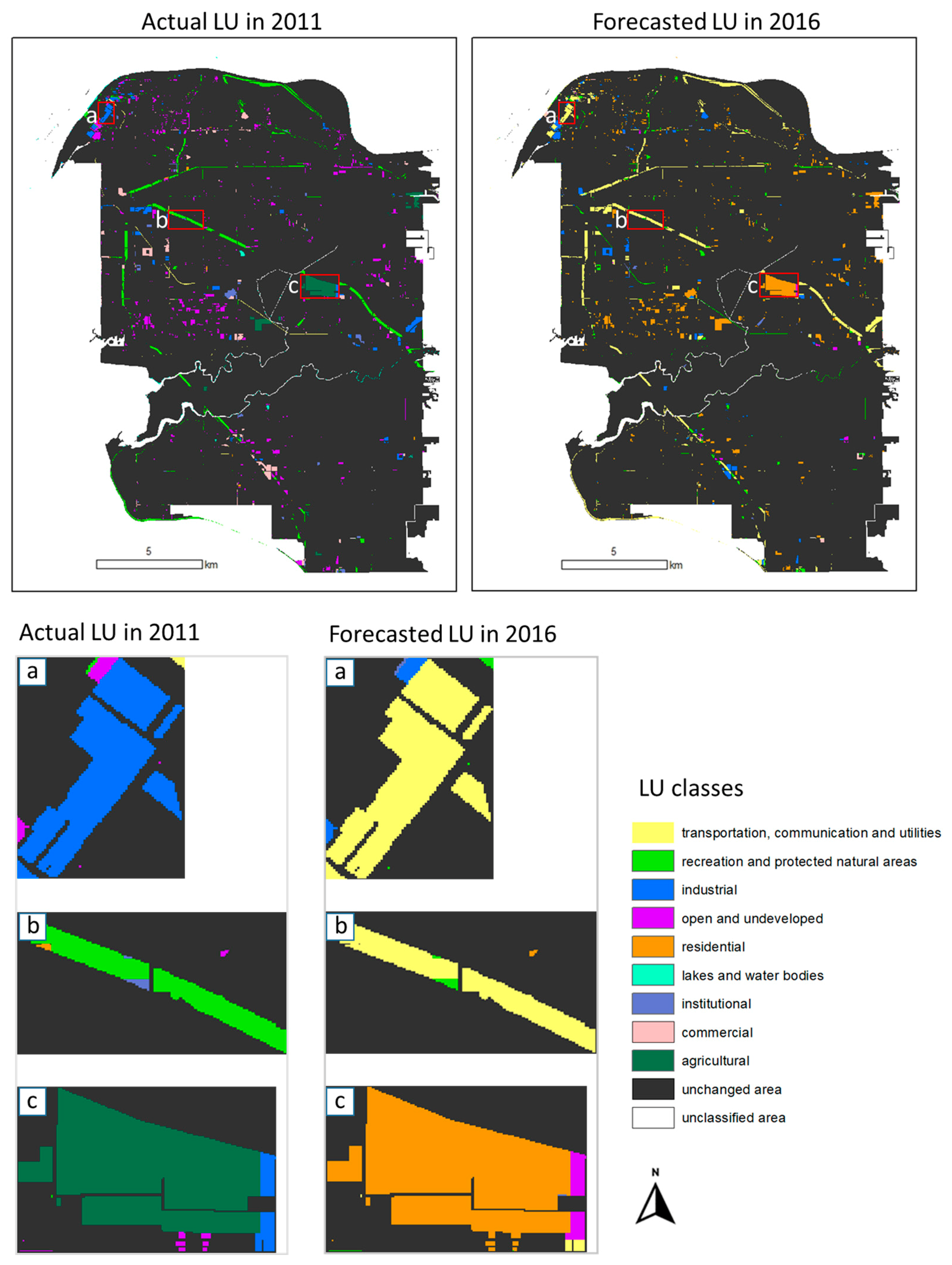
Figure 6 shows the obtained LU for the City of Surrey for the year 2016, generated by short-term forecast using LSTM 2, which was trained by using all raster cells from the study area. The percentages of each LU class as forecasted are: 10.71% transportation, communication, and utilities, 9.25% recreation and protected natural areas, 2.87% industrial, 2.13% open and undeveloped, 22.99% residential, 0.02% lakes and water bodies, 0.92% institutional, 0.99% commercial, and 16.01% agricultural. As forecasted, only 4.5% of raster cells changed their LU classes compared with the 2011 LU. Figure 7 shows the changed raster cells in 2011 and 2016; it can be seen that some industrial land in the northwest part of the study area became transportation, and some open areas become industrial (Figure 7a). Some of the natural and protected areas were predicted as transportation LU class (Figure 7b), while some of the agricultural areas were forecasted as residential (Figure 7c). Based on the prediction, the increased LU classes during 2011 and 2016 were transportation and residential, while the other LUs decreased. Specifically, 28.1% of changed raster cells changed from recreational and protected natural LUs to transportation LUs, 11.9% of changed cells with agricultural LUs turned into residential LUs, 18.6% undeveloped and open LUs became residential LUs, and 6.1% of commercial LUs became industrial LUs.
Figure 8 presents the confusion matrix for the first group of 604 sample points; it was calculated based on Ytrue() and Ypred(). The rows indicated the target LU classes Ytrue() that were manually classified from sample location () on the 2016 orthophoto. The columns indicated the predicted LU classes Ypred() at corresponding sample locations (i = 1,2,3…604) from the forecasted model outputs. Moreover, the confusion matrix value of cell (i,j) (i,j = 1,2,3…9), where 1–9 indicate number of LU classes, represents the percentage of LU class j that was forecasted as class i. The total accuracy of LU forecast is 87%, while the TN, TP, FN, and FP of LU forecast in each LU class differs. Especially, the true negative from LU classes such as “open and undeveloped land” and “lakes and water bodies”, and “commercial” are low, close to 50%. The percentage of “water bodies” decreased, while the percentage of “residential” and “agricultural” increased, as indicated in confusion matrix.
An additional 408 randomly selected sampling points from the orthophoto image for the year 2016 were selected to correspond only to the changed raster cells from the 2011 actual and 2016 forecasted LUC. Each sample point on the orthophoto image was manually classified and considered as actual LU class of the year 2016. Then, they were compared with the forecasted LU class at corresponding raster cells. The obtained overall accuracy for changed raster cells is 25%. The residential and institutional LU classes were correctly forecasted with 45% and 40% accuracy respectively, while the other LU classes were forecasted with very low accuracy, ranging from 5% to 15%. According to the obtained results, the overall amount of changed raster cells were overestimated; however, the residential and institutional LUs were steadily increasing, as open and undeveloped LU. The results still correspond to the situation of the increasing population in the City of Surrey, thus increasing urban development.
4. Discussion and Conclusions
LUC is a spatiotemporal phenomenon and it can be correlated with various factors. Consequently, forecasting LUC is a challenging topic and extensive efforts have been dedicated to modeling LUC, while only a few studies have explored the potential of DL models on this topic. While RNN has been shown as an efficient approach to solve time-series data, the objective of this study was to test the feasibility of RNN based models for short-term LUC forecasting.
This study successfully tested several RNN based models to examine the LUC of the City of Surrey. The LSTM, GRU, BiLSTM, and ConvLSTM were trained by changed raster cells and persistent raster cells. Then, the LU for the year 2016 was forecasted using LSTM, which was trained first by LU data for years 1996, 2001, 2006, and 2011 at 10-meter spatial and 5-year temporal resolutions.
The RNNs were successfully trained by LU data, as well as being able to forecast the 2016 LU. The training data have layers of most frequent LU in the Moore neighborhood to account for the impact from local surrounding raster cells. The model accuracy turns out to be similar at 86% while trained by both changed and persistent raster cells. Model accuracy was lower at 62% when trained by only changed cells, which indicates the variants of RNN did not differ much when using the same LU datasets. The forecasted results indicate that only 4.5% of the land in Surrey City had changed. Overall, the forecasted changes mainly occurred among industrial, natural and recreational, transportation, open and undeveloped, agricultural, and residential LU classes. However, among the changed raster cells, only 25% of the LUC was forecasted correctly when evaluating sample points only from the changed raster cells. The results indicate that the land was not overdeveloped between 2011 and 2016 while the City of Surrey experienced an increase in population, and some unpredictable factors may have influenced the LUC. The obtained overall low accuracy of the changed raster cells can be related to the lack of a larger number of geospatial datasets that span across multiple years, which could make DL methods more inefficient; the absence of actual LU data for the forecasted year, as manual classification of orthophoto could contain errors; and, finally, the difficulty for these type of models to capture human interventions such as decision making for land management.
Due to the limitation of availability of classified LU data for 2016, in this study the forecasted LUC for the year 2016 was not fully validated. Instead, it was compared with the actual 2011 LU data and the locations with LU changes were analyzed. The LSTM can estimate how each LU will change based on “transition rules”, which were learned from the 1996 to 2011 LU data. In addition, manually classified 2016 orthophoto data were used to verify the obtained forecasted LUC. The Kappa statistic [96] is often used as an assessment indicator to compare the similarity between observed and predicted results [45,100]. Given that the majority of the raster cells remain unchanged, simple random sampling (SRS) is not sufficient to evaluate the overall predication performance of the RNN models since the overall accuracy will be increased by the unchanged raster cells. Instead, other sampling methods [101,102] could potentially be used to evaluate the obtained forecasted LUC. However, if the appropriate LU data were available for the year 2016, the evaluation of the accuracy of the obtained short-term forecasted LUC could be performed with a variety of exiting methods for map comparisons [95,103,104].
RNNs are efficient methods capable of performing feature extraction and classification. So far, few studies have exploited RNNs for LUC forecasting. This research study has demonstrated that RNNs have this potential, although the performance of LU forecasting still needs appropriate geospatial data so that strict validation can be performed. RNNs are data-driven models, the quality and quantity of the training data are important factors determining the accuracy of the forecasting results. Thus, training the models represents a challenge when such models are used. Incorporating proximate physical, local, demographic, socioeconomic, and climatic factors into the training process, the RNNs can better learn the transition rules and improve the forecast accuracy. However, not every type of data is available and open to the public.
In summary, in this study RNNs facilitated the full automation of the LU modeling process from available geospatial datasets due to the learning abilities of RNNs. Expert knowledge is not required to initialize the models and interpret the results. RNNs have the potential to capture the spatio-temporal patterns of LUC and provide consistent short-term forecasts. The RNNs could become a suitable approach for LUC modeling, thus also be a useful tool to study LUC and to further inform decision-makers in their land use management process.
Author Contributions
Data curation, C.C.; formal analysis, C.C., S.D. and S.L.; investigation, C.C. and S.D.; writing—original draft, review and editing, C.C. and S.D.; writing—review and editing, S.L.
Funding
This research was funded by Natural Sciences and Engineering Research Council (NSERC) of Canada Discovery Grants RGPIN-2017-03939 and RGPIN-2017-05950 awarded respectively to the second and third authors.
Acknowledgments
The authors are thankful to the Natural Sciences and Engineering Research Council (NSERC) of Canada Discovery Grants program for the full support of this research study. The authors appreciate valuable and constructive feedback from the four anonymous reviewers. Special thanks to SFU Open Access Fund for sponsoring the publication of this paper in the open access journal.
Conflicts of Interest
The authors declare no conflicts of interest.
References
- Kleemann, J.; Baysal, G.; Bulley, H.N.N.; Fürst, C. Assessing driving forces of land use and land cover change by a mixed-method approach in north-eastern Ghana, West Africa. J. Environ. Manag. 2017, 196, 411–442. [Google Scholar] [CrossRef] [PubMed]
- de Palma, A.; Sanchez-Ortiz, K.; Martin, P.A.; Chadwick, A.; Gilbert, G.; Bates, A.E.; Börger, L.; Contu, S.; Hill, S.L.L.; Purvis, A. Challenges with Inferring How Land-Use Affects Terrestrial Biodiversity: Study Design, Time, Space and Synthesis. In Advances in Ecological Research; Bohan, D.A., Dumbrell, A.J., Woodward, G., Jackson, M., Eds.; Academic Press: Cambridge, MA, USA, 2018; pp. 163–199. [Google Scholar]
- Green, K.; Kempka, D.; Lackey, L. Using Remote Sensing to Detect and Monitor Land-Cover and Land-Use Change. Am. Soc. Photogramm. Remote Sensine. 1994, 60, 331–337. [Google Scholar]
- Anderson, J.R.; Hardy, E.E.; Roach, J.T.; Witmer, R.E. A Land Use and Land Cover Classification System for Use with Remote Sensor Data; Professional Paper; USGS Numbered Series 964; 1976. Available online: https://pubs.er.usgs.gov/publication/pp964 (accessed on 24 May 2019).
- National Research Council. Advancing Land Change Modeling: Opportunities and Research Requirements; The National Academies Press: Washington, DC, USA, 2014. [Google Scholar]
- Fukushima, K. Neocognitron: A self-organizing neural network model for a mechanism of pattern recognition unaffected by shift in position. Biol. Cybern. 1980, 36, 193–202. [Google Scholar] [CrossRef] [PubMed]
- Rumelhart, D.E.; Hinton, G.E.; Williams, R.J. Learning representations by back-propagating errors. Nature 1986, 323, 533. [Google Scholar] [CrossRef]
- Schmidhuber, J. History of computer vision contests won by deep CNNs on GPUs. March 2017. Available online: http://people.idsia.ch/~juergen/computer-vision-contests-won-by-gpu-cnns.html (accessed on 24 May 2019).
- Huang, B.; Zhao, B.; Song, Y. Urban land-use mapping using a deep convolutional neural network with high spatial resolution multispectral remote sensing imagery. Remote Sens. Environ. 2018, 214, 73–86. [Google Scholar] [CrossRef]
- Graves, A.; Mohamed, A.; Hinton, G. Speech recognition with deep recurrent neural networks. In Proceedings of the 2013 IEEE International Conference on Acoustics, Speech and Signal Processing, Vancouver, BC, Canada, 26–31 May 2013; pp. 6645–6649. [Google Scholar]
- Mahoney, M. Large Text Compression Benchmark. 2017. Available online: http://www.mattmahoney.net/dc/text.html#1218 (accessed on 24 May 2019).
- Yao, Y.; Li, X.; Liu, X.; Liu, P.; Liang, Z.; Zhang, J.; Mai, K. Sensing Spatial Distribution of Urban Land Use by Integrating Points-of-interest and Google Word2Vec Model. Int. J. Geogr. Inf. Sci. 2017, 31, 825–848. [Google Scholar] [CrossRef]
- Yao, Y.; Liang, H.; Li, X.; Zhang, J.; He, J. Sensing Urban Land-Use Patterns By Integrating Google Tensorflow And Scene-Classification Models. Int. Arch. Photogramm. Remote Sens. Spatial Inf. Sci. 2017, XLII-2-W7. [Google Scholar] [CrossRef]
- Liu, J.; Shahroudy, A.; Xu, D.; Kot, A.C.; Wang, G. Skeleton-Based Action Recognition Using Spatio-Temporal LSTM Network with Trust Gates. IEEE Trans. Pattern Anal. Mach. Intell. 2018, 40, 3007–3021. [Google Scholar] [CrossRef] [PubMed]
- Hegazy, I.R.; Kaloop, M.R. Monitoring urban growth and land use change detection with GIS and remote sensing techniques in Daqahlia governorate Egypt. Int. J. Sustain. Built Environ. 2015, 4, 117–124. [Google Scholar] [CrossRef] [Green Version]
- Kumar, S.; Radhakrishnan, N.; Mathew, S. Land use change modelling using a Markov model and remote sensing. Geomat. Nat. Hazards Risk. 2014, 5, 145–156. [Google Scholar] [CrossRef]
- Muller, M.R.; Middleton, J. A Markov model of land-use change dynamics in the Niagara Region, ON, Canada. Landsc. Ecol. 1994, 9, 151–157. [Google Scholar]
- Batty, M.; Xie, Y. From Cells to Cities. Environ. Plann. B Plann. Des. 1994, 21, S31–S48. [Google Scholar] [CrossRef]
- Clarke, K.C.; Hoppen, S.; Gaydos, L. A Self-Modifying Cellular Automaton Model of Historical Urbanization in the San Francisco Bay Area. Environ. Plann. B Plann. Des. 1997, 24, 247–261. [Google Scholar] [CrossRef]
- Clarke, K.C.; Gaydos, L.J. Loose-coupling a cellular automaton model and GIS: Long-term urban growth prediction for San Francisco and Washington/Baltimore. Int. J. Geogr. Inf. Sci. 1998, 12, 699–714. [Google Scholar] [CrossRef] [PubMed]
- White, R.; Engelen, G. Cellular Automata as the Basis of Integrated Dynamic Regional Modelling. Environ. Plann. B Plann. Des. 1997, 24, 235–246. [Google Scholar] [CrossRef]
- Wu, F.; Webster, C.J. Simulation of Land Development through the Integration of Cellular Automata and Multicriteria Evaluation. Environ. Plann. B Plann. Des. 1998, 25, 103–126. [Google Scholar] [CrossRef]
- Li, X.; Yeh, A.G.-O. Neural-network-based cellular automata for simulating multiple land use changes using GIS. Int. J. Geogr. Inf. Sci. 2002, 16, 323–343. [Google Scholar] [CrossRef]
- Lin, H.; Lu, K.S.; Espey, M.; Allen, J. Modeling Urban Sprawl and Land Use Change in a Coastal Area-- A Neural Network Approach; 2005 Annual meeting, July 24–27, Providence, RI; 19364; American Agricultural Economics Association (New Name 2008: Agricultural and Applied Economics Association). 2005. Available online: https://www.semanticscholar.org/paper/Modeling-Urban-Sprawl-and-Land-Use-Change-in-a-Area-Lin-Lu/3a504a2df02f3353efde7b30ff9b9bd96bfdc0a1 (accessed on 29 May 2019).
- Pijanowski, B.C.; Brown, D.G.; Shellito, B.A.; Manik, G.A. Using neural networks and GIS to forecast land use changes: A Land Transformation Model. Comput. Environ. Urban Syst. 2002, 26, 553–575. [Google Scholar] [CrossRef]
- Cheng, J.; Masser, I. Urban growth pattern modeling: A case study of Wuhan city, PR China. Landsc. Urban Plan. 2003, 62, 199–217. [Google Scholar] [CrossRef]
- Brown, D.G.; Page, S.; Riolo, R.; Zellner, M.; Rand, W. Path dependence and the validation of agent-based spatial models of land use. Int. J. Geogr. Inf. Sci. 2005, 19, 153–174. [Google Scholar] [CrossRef]
- Sanders, L.; Pumain, D.; Mathian, H.; Guérin-Pace, F.; Bura, S. SIMPOP: A Multiagent System for the Study of Urbanism. Environ. Plann. B Plann. Des. 1997, 24, 287–305. [Google Scholar] [CrossRef]
- Huang, B.; Xie, C.; Tay, R.; Wu, B. Land-use-change modeling using unbalanced support-vector machines. Environ. Plan. B Plan. Des. 2009, 36, 398–416. [Google Scholar] [CrossRef]
- Nemmour, H.; Chibani, Y. Multiple support vector machines for land cover change detection: An application for mapping urban extensions. ISPRS J. Photogramm. Remote Sens. 2006, 61, 125–133. [Google Scholar] [CrossRef]
- Otukei, J.R.; Blaschke, T. Land cover change assessment using decision trees, support vector machines and maximum likelihood classification algorithms. Int. J. Appl. Earth Obs. Geoinf. 2010, 12, S27–S31. [Google Scholar] [CrossRef]
- Samardzic-Petrovic, M.; Dragicevic, S.; Kovacevic, M.; Bajat, B. Modeling Urban Land Use Changes Using Support Vector Machines. Trans. GIS. 2016, 20, 718–734. [Google Scholar] [CrossRef]
- Chaudhuri, G.; Clarke, K. The SLEUTH land use change model: A review. Int. J. Environ. Resour. Res. 2013, 1, 88–105. [Google Scholar]
- White, R.; Engelen, G.; Uljee, I. The Use of Constrained Cellular Automata for High-Resolution Modelling of Urban Land-Use Dynamics. Environ. Plann. B Plann. Des. 1997, 24, 323–343. [Google Scholar] [CrossRef]
- Batty, M.; Xie, Y.; Sun, Z. Modeling urban dynamics through GIS-based cellular automata. Comput. Environ. Urban Syst. 1999, 23, 205–233. [Google Scholar] [CrossRef] [Green Version]
- Stevens, D.; Dragićević, S. A GIS-Based Irregular Cellular Automata Model of Land-Use Change. Environ. Plan. B Plan. Des. 2007, 34, 708–724. [Google Scholar] [CrossRef]
- Guan, D.; Li, H.; Inohae, T.; Su, W.; Nagaie, T.; Hokao, K. Modeling urban land use change by the integration of cellular automaton and Markov model. Ecol. Model. 2011, 222, 3761–3772. [Google Scholar] [CrossRef]
- Samardzic-Petrovic, M.; Kovačević, M.; Bajat, B.; Dragićević, S. Machine Learning Techniques for Modelling Short Term Land-Use Change. ISPRS Int. J. Geo-Inf. 2017, 6, 387. [Google Scholar] [CrossRef]
- Samardžić-Petrović, M.; Dragićević, S.; Bajat, B.; Kovačević, M. Exploring the Decision Tree Method for Modelling Urban Land Use Change. Geomatica 2015, 69, 313–325. [Google Scholar] [CrossRef]
- Arel, I.; Rose, D.C.; Karnowski, T.P. Deep Machine Learning—A New Frontier in Artificial Intelligence Research. IEEE Comput. Intell. Mag. 2010, 5, 13–18. [Google Scholar] [CrossRef]
- Mukherjee, S.; Shashtri, S.; Singh, C.K.; Srivastava, P.K.; Gupta, M. Effect of canal on land use/land cover using remote sensing and GIS. J. Indian Soc. Remote Sens. 2009, 37, 527–537. [Google Scholar] [CrossRef]
- Lipton, Z. A Critical Review of Recurrent Neural Networks for Sequence Learning. 2015. Available online: http://zacklipton.com/media/papers/recurrent-network-review-lipton-2015v2.pdf (accessed on 29 May 2019).
- Byeon, W.; Breuel, T.M.; Raue, F.; Liwicki, M. Scene labeling with LSTM recurrent neural networks. In Proceedings of the 2015 IEEE Conference on Computer Vision and Pattern Recognition (CVPR), Boston, MA, USA, 7–12 June 2015; pp. 3547–3555. [Google Scholar]
- Rußwurm, M.; Körner, M. Multi-Temporal Land Cover Classification with Long Short-Term Memory Neural Networks. ISPRS—Int. Arch. Photogramm. Remote Sens. Spatial Inf. Sci. 2017, XLII-1/W1, 551–558. [Google Scholar]
- Rußwurm, M.; Körner, M. Temporal Vegetation Modelling using Long Short-Term Memory Networks for Crop Identification from Medium-Resolution Multi-Spectral Satellite Image. In Proceedings of the 2017 IEEE Conference on Computer Vision and Pattern Recognition Workshops (CVPRW), Honolulu, HI, USA, 21–26 July 2017. [Google Scholar]
- Bengio, Y. Learning Deep Architectures for AI. MAL 2009, 2, 1–127. [Google Scholar] [CrossRef]
- Ienco, D.; Gaetano, R.; Dupaquier, C.; Maurel, P. Land Cover Classification via Multitemporal Spatial Data by Deep Recurrent Neural Networks. IEEE Geosci. Remote Sens. Lett. 2017, 14, 1685–1689. [Google Scholar] [CrossRef] [Green Version]
- Rußwurm, M.; Körner, M. Multi-Temporal Land Cover Classification with Sequential Recurrent Encoders. ISPRS Int. J. Geo-Inf. 2018, 7, 129. [Google Scholar] [Green Version]
- Sharma, A.; Liu, X.; Yang, X. Land cover classification from multi-temporal, multi-spectral remotely sensed imagery using patch-based recurrent neural networks. Neural Netw. 2018, 105, 346–355. [Google Scholar] [CrossRef] [Green Version]
- Lyu, H.; Lu, H.; Mou, L. Learning a Transferable Change Rule from a Recurrent Neural Network for Land Cover Change Detection. Remote Sens. 2016, 8, 506. [Google Scholar] [CrossRef]
- Mou, L.; Zhu, X.X. A Recurrent Convolutional Neural Network for Land Cover Change Detection in Multispectral Images. In Proceedings of the IGARSS 2018—2018 IEEE International Geoscience and Remote Sensing Symposium, Valencia, Spain, 22–27 July 2018; pp. 4363–4366. [Google Scholar]
- Du, G.; Yuan, L.; Shin, K.J.; Managi, S. Modeling the Spatio-Temporal Dynamics of Land Use Change with Recurrent Neural Networks. 2018. Available online: https://arxiv.org/abs/1803.10915 (accessed on 29 May 2019).
- McCulloch, W.S.; Pitts, W. A logical calculus of the ideas immanent in nervous activity. Bull. Math. Biophys. 1943, 5, 115–133. [Google Scholar] [CrossRef]
- Graves, A. Supervised Sequence Labelling with Recurrent Neural Networks; Springer: Berlin/Heidelberg, Germany, 2012; Volume 385. [Google Scholar]
- Eck, D.; Schmidhuber, J. Learning the Long-Term Structure of the Blues. In Proceedings of the Artificial Neural Networks—ICANN 2002, Madrid, Spain, 28–30 August 2002. [Google Scholar]
- Graves, A.; Schmidhuber, J.; Koller, D.; Schuurmans, D.; Bengio, Y.; Bottou, L. Offline Handwriting Recognition with Multidimensional Recurrent Neural Networks. In Advances in Neural Information Processing Systems 21; Curran Associates, Inc.: Dutchess County, NY, USA, 2009; pp. 545–552. Available online: https://papers.nips.cc/paper/3449-offline-handwriting-recognition-with-multidimensional-recurrent-neural-networks (accessed on 16 August 2019).
- Zen, H.; Sak, H. Unidirectional long short-term memory recurrent neural network with recurrent output layer for low-latency speech synthesis. In Proceedings of the 2015 IEEE International Conference on Acoustics, Speech and Signal Processing (ICASSP), South Brisbane, Australia, 19–24 April 2015; pp. 4470–4474. [Google Scholar]
- Yang, Y.; Zhou, J.; Ai, J.; Bin, Y.; Hanjalic, A.; Shen, H.T.; Ji, Y. Video Captioning by Adversarial LSTM. IEEE Trans. Image Process. 2018, 27, 5600–5611. [Google Scholar] [CrossRef] [PubMed]
- Nelson, D.M.Q.; Pereira, A.M.; de Oliveira, R.A. Stock market’s price movement prediction with LSTM neural networks. In Proceedings of the 2017 International Joint Conference on Neural Networks (IJCNN), Anchorage, Alaska, 14–19 May 2017; pp. 1419–1426. [Google Scholar]
- Qing, X.; Niu, Y. Hourly day-ahead solar irradiance prediction using weather forecasts by LSTM. Energy 2018, 148, 461–468. [Google Scholar] [CrossRef]
- Fernandes, B.; Silva, F.; Alaiz-Moretón, H.; Novais, P.; Analide, C.; Neves, J. Traffic Flow Forecasting on Data-Scarce Environments Using ARIMA and LSTM Networks. In Proceedings of the New Knowledge in Information Systems and Technologies, La Toja, Spain, 16–19 April 2019; pp. 273–282. [Google Scholar]
- Han, Y.; Wang, C.; Ren, Y.; Wang, S.; Zheng, H.; Chen, G. Short-Term Prediction of Bus Passenger Flow Based on a Hybrid Optimized LSTM Network. Isprs Int. J. Geo-Inf. 2019, 8, 366. [Google Scholar] [CrossRef]
- Bengio, Y.; Simard, P.; Frasconi, P. Learning long-term dependencies with gradient descent is difficult. IEEE Trans. Neural Netw. 1994, 5, 157–166. [Google Scholar] [CrossRef]
- Hochreiter, S.; Schmidhuber, J. Long Short-Term Memory. Neural Comput. 1997, 9, 1735–1780. [Google Scholar] [CrossRef] [PubMed]
- Cho, K.; Van Merriënboer, B.; Gulcehre, C.; Bahdanau, D.; Bougares, F.; Schwenk, H.; Bengio, Y. Learning Phrase Representations using RNN Encoder–Decoder for Statistical Machine Translation. In Proceedings of the 2014 Conference on Empirical Methods in Natural Language Processing (EMNLP), Doha, Qatar, 25–29 October 2014; pp. 1724–1734. [Google Scholar]
- Chung, J.; Gulcehre, C.; Cho, K.; Bengio, Y. Empirical evaluation of gated recurrent neural networks on sequence modeling. In Proceedings of the NIPS 2014 Workshop on Deep Learning, Montreal, QC, Canada, 12 December 2014. [Google Scholar]
- Schuster, M.; Paliwal, K.K. Bidirectional recurrent neural networks. IEEE Trans. Signal Process. 1997, 45, 2673–2681. [Google Scholar] [CrossRef] [Green Version]
- Graves, A.; Jaitly, N.; Mohamed, A. Hybrid speech recognition with Deep Bidirectional LSTM. In Proceedings of the 2013 IEEE Workshop on Automatic Speech Recognition and Understanding, Olomouc, Czech Republic, 8–12 December 2013; pp. 273–278. [Google Scholar]
- Graves, A.; Fernández, S.; Schmidhuber, J. Bidirectional LSTM Networks for Improved Phoneme Classification and Recognition. In Proceedings of the Artificial Neural Networks: Formal Models and Their Applications—ICANN 2005, Warsaw, Poland, 11–15 September 2005; pp. 799–804. [Google Scholar]
- Shi, X.; Chen, Z.; Wang, H.; Yeung, D.-Y.; Wong, W.; Woo, W. Convolutional LSTM Network: A Machine Learning Approach for Precipitation Nowcasting. In Advances in Neural Information Processing Systems 28; Cortes, C., Lawrence, N.D., Lee, D.D., Sugiyama, M., Garnett, R., Eds.; Curran Associates, Inc.: Dutchess County, NY, USA, 2015; pp. 802–810. Available online: https://papers.nips.cc/paper/5955-convolutional-lstm-network-a-machine-learning-approach-for-precipitation-nowcasting (accessed on 16 August 2019).
- Yuan, Z.; Zhou, X.; Yang, T. Hetero-ConvLSTM: A Deep Learning Approach to Traffic Accident Prediction on Heterogeneous Spatio-Temporal Data. In Proceedings of the 24th ACM SIGKDD International Conference on Knowledge Discovery & Data Mining, London, UK, 19–23 August 2018; pp. 984–992. [Google Scholar]
- Luo, W.; Liu, W.; Gao, S. Remembering history with convolutional LSTM for anomaly detection. In Proceedings of the 2017 IEEE International Conference on Multimedia and Expo (ICME), Hong Kong, China, 10–14 July 2017; pp. 439–444. [Google Scholar]
- Liu, Y.; Zheng, H.; Feng, X.; Chen, Z. Short-term traffic flow prediction with Conv-LSTM. In Proceedings of the 9th International Conference on Wireless Communications and Signal Processing (WCSP), Nanjing, China, 11–13 October 2017; pp. 1–6. [Google Scholar]
- Fan, B.; Wang, L.; Soong, F.K.; Xie, L. Photo-real talking head with deep bidirectional LSTM. In Proceedings of the 2015 IEEE International Conference on Acoustics, Speech and Signal Processing (ICASSP), South Brisbane, Australia, 19–24 April 2015; pp. 4884–4888. [Google Scholar]
- Lv, Z.; Xu, J.; Zheng, K.; Yin, H.; Zhao, P.; Zhou, X. LC-RNN: A Deep Learning Model for Traffic Speed Prediction. In Proceedings of the Twenty-Seventh International Joint Conference on Artificial Intelligence, IJCAI-18, Stockholm, Sweden, 13–19 July 2018. [Google Scholar] [CrossRef]
- Li, S.; Li, W.; Cook, C.; Zhu, C.; Gao, Y. Independently Recurrent Neural Network (IndRNN): Building A Longer and Deeper RNN. In Proceedings of the 2018 IEEE/CVF Conference on Computer Vision and Pattern Recognition, Salt Lake City, UT, USA, 18–23 June 2018. [Google Scholar] [CrossRef]
- Jeblad. Gradient Recurrent Unit, fully gated version. In Based on Example in Recurrent Neural Network (RNN)—Part 5: Custom Cells. 2018. Available online: https://commons.wikimedia.org/wiki/File:Gated_Recurrent_Unit,_base_type.svg (accessed on 16 August 2019).
- Cui, Z.; Ke, R.; Wang, Y. Deep Stacked Bidirectional and Unidirectional LSTM Recurrent Neural Network for Network-Wide Traffic Speed Prediction. IEEE 2018, 12. Available online: https://arxiv.org/abs/1801.02143 (accessed on 16 August 2019).
- Colah. Understanding LSTM Networks. 2015. Available online: https://colah.github.io/posts/2015-08-Understanding-LSTMs/ (accessed on 16 August 2019).
- City of Surrey. Population Estimates & Projections. 2018. Available online: http://www.surrey.ca/business-economic-development/1418.aspx (accessed on 24 May 2019).
- City of Surrey. 2019. Available online: http://www.surrey.ca/default.aspx (accessed on 17 May 2019).
- Vancouver, M. Open Data Catalogue. Metro Vancouver. 2011. Available online: http://www.metrovancouver.org/data (accessed on 21 December 2018).
- DMTI Spatial Inc. CanMap Streetfiles. 2011. Available online: https://www.dmtispatial.com/canmap/ (accessed on 24 May 2019).
- ESRI. ArcGIS Desktop Version 10.6; ESRI: Redlands, CA, USA, 2018. [Google Scholar]
- Karpathy, A. The Unreasonable Effectiveness of Recurrent Neural Networks. Andrej Karpathy Blog, 21 May 2015. [Google Scholar]
- Rubinstein, R.Y.; Kroese, D.P. The Cross-Entropy Method: A Unified Approach to Combinatorial Optimization, Monte-Carlo Simulation and Machine Learning; Springer: New York, NY, USA, 2004. [Google Scholar]
- Bishop, C.M. Pattern Recognition and Machine Learning; Springer: New York, NY, USA, 2016. [Google Scholar]
- Bridle, J.S. Probabilistic Interpretation of Feedforward Classification Network Outputs, with Relationships to Statistical Pattern Recognition; Springer: Berlin/Heidelberg, Germany, 1990; pp. 227–236. [Google Scholar]
- Box, G.E.P.; Meyer, R.D. An Analysis for Unreplicated Fractional Factorials. Technometrics 1986, 28, 11–18. [Google Scholar] [CrossRef]
- Guyon, I. A Scaling Law for the Validation-Set Training-Set Size Ratio. Available online: http://citeseerx.ist.psu.edu/viewdoc/download?doi=10.1.1.33.1337&rep=rep1&type=pdf (accessed on 16 August 2019).
- Gholami, V.; Chau, K.W.; Fadaie, F.; Torkaman, J.; Ghaffari, A. Modeling of groundwater level fluctuations using dendrochronology in alluvial aquifers. J. Hydrol. 2015, 529, 1060–1069. [Google Scholar] [CrossRef]
- City of Surrey. Imagery—City of Surrey Open Data Catalogue. 2017. Available online: http://data.surrey.ca/group/6878e307-9fec-4134-b042-d7e058310255?tags=orthophoto (accessed on 10 September 2018).
- Isreal, G.D. Determining Sample Size; Institute of Food and Agricultural Sciences (IFAS), University of Florida: Gainesville, FL, USA, 1992. [Google Scholar]
- Cohen, J. A Coefficient of Agreement for Nominal Scales. Educ. Psychol. Meas. 1960, 20, 37–46. [Google Scholar] [CrossRef]
- Stehman, S.V. Selecting and interpreting measures of thematic classification accuracy. Remote Sens. Environ. 1997, 62, 77–89. [Google Scholar] [CrossRef]
- Congalton, R.G. A review of assessing the accuracy of classifications of remotely sensed data. Remote Sens. Environ. 1991, 37, 35–46. [Google Scholar] [CrossRef]
- The MathWorks Inc. MATLAB R2018a; The MathWorks Inc.: Natick, MA, USA, 2018. [Google Scholar]
- Python Software Foundation. Python Language Reference, Version 3.6. 2016. Available online: http://www.python.org (accessed on 29 May 2019).
- Fran, C. Keras. 2015. Available online: https://keras.io/ (accessed on 29 May 2019).
- Monserud, R.A.; Leemans, R. Comparing global vegetation maps with the Kappa statistic. Ecol. Model. 1992, 62, 275–293. [Google Scholar] [CrossRef]
- Hashemian, M.; Abkar, A.; Fatemi, S. Study of Sampling Methods for Accuracy Assessment of Classified Remotely Sensed Data. 2004. Available online: https://pdfs.semanticscholar.org/0fac/07aef155bfae046e21ebb7d7f50b612ec168.pdf (accessed on 16 August 2019).
- Mu, X.; Hu, M.; Song, W.; Ruan, G.; Ge, Y.; Wang, J.; Huang, S.; Yan, G. Evaluation of Sampling Methods for Validation of Remotely Sensed Fractional Vegetation Cover. Remote Sens. 2015, 7, 16164–16182. [Google Scholar] [CrossRef] [Green Version]
- Pontius, R.G., Jr.; Millones, M. Death to Kappa: Birth of quantity disagreement and allocation disagreement for accuracy assessment. Int. J. Remote Sens. 2011, 32, 4407–4429. [Google Scholar] [CrossRef]
- Visser, H.; de Nijs, T. The Map Comparison Kit. Environ. Model. Softw. 2006, 21, 346–358. [Google Scholar] [CrossRef]
Figure 1.
A recurrent neural network (RNN) [7] structure allowing information to loop in the layer, and it can be unfolded as a neural network indicated at the right side. is a temporal sequence input. is the hidden state.
Figure 1.
A recurrent neural network (RNN) [7] structure allowing information to loop in the layer, and it can be unfolded as a neural network indicated at the right side. is a temporal sequence input. is the hidden state.

Figure 2.
Structure of the convolutional long-short term memory (ConvLSTM) [70] model with (a) transforming 2D image into 3D tensor and (b) its inner structure and the structure of (c) the gated recurrent unit (GRU) [77] and (d) bidirectional LTSM (BiLSTM) [78] models.

Figure 3.
The graphical representation of an LSTM layer [79].
Figure 3.
The graphical representation of an LSTM layer [79].

Figure 4.
The City of Surrey located in the south of the Metro Vancouver Region.

Figure 5.
The flowchart of the proposed LSTM models for land use change (LUC) forecast, where LU data were considered for years t-5 = 1996, t = 2001, t + 5 = 2006 and t + 10 = 2011 for training and validation of the LSTM and then forecasted for t + 15 = 2016.
Figure 5.
The flowchart of the proposed LSTM models for land use change (LUC) forecast, where LU data were considered for years t-5 = 1996, t = 2001, t + 5 = 2006 and t + 10 = 2011 for training and validation of the LSTM and then forecasted for t + 15 = 2016.

Figure 6.
LU classes for 2016 for the City of Surrey generated by LSTM 2 model.

Figure 7.
Changed LU raster cells in 2011 as actual and 2016 as forecasted obtained by LSTM with detailed subsections (a–c) as examples.
Figure 7.
Changed LU raster cells in 2011 as actual and 2016 as forecasted obtained by LSTM with detailed subsections (a–c) as examples.

Figure 8.
Confusion matrix based on the comparison of the forecasted LU and orthophotos for the year 2016.
Figure 8.
Confusion matrix based on the comparison of the forecasted LU and orthophotos for the year 2016.


Table 1.
The training and validation accuracy of different RNN models and scenarios.
| Scenarios | RNN Variants | The Ratio of Changed Raster Cells in Training Set | Training Accuracy | Validation Accuracy |
|---|---|---|---|---|
| (1) | LSTM 1 | 100% | 0.62 | 0.62 |
| (2) | LSTM 2 | 47% | 0.87 | 0.87 |
| (3) | GRU | 47% | 0.86 | 0.87 |
| (4) | BiLSTM | 47% | 0.87 | 0.87 |
| (5) | ConvLSTM 1, 10 × 10 | 47% | 0.88 | 0.88 |
| (6) | ConvLSTM 2, 5 × 5 | 47% | 0.88 | 0.88 |
© 2019 by the authors. Licensee MDPI, Basel, Switzerland. This article is an open access article distributed under the terms and conditions of the Creative Commons Attribution (CC BY) license (http://creativecommons.org/licenses/by/4.0/).
Share and Cite
MDPI and ACS Style
Cao, C.; Dragićević, S.; Li, S. Short-Term Forecasting of Land Use Change Using Recurrent Neural Network Models. Sustainability 2019, 11, 5376. https://doi.org/10.3390/su11195376
AMA Style
Cao C, Dragićević S, Li S. Short-Term Forecasting of Land Use Change Using Recurrent Neural Network Models. Sustainability. 2019; 11(19):5376. https://doi.org/10.3390/su11195376
Chicago/Turabian StyleCao, Cong, Suzana Dragićević, and Songnian Li. 2019. "Short-Term Forecasting of Land Use Change Using Recurrent Neural Network Models" Sustainability 11, no. 19: 5376. https://doi.org/10.3390/su11195376
Note that from the first issue of 2016, this journal uses article numbers instead of page numbers. See further details here.