Article

A CBR–AHP Hybrid Method to Support the Decision-Making Process in the Selection of Environmental Management Actions

by
Fernando Ramos-Quintana
1,*,
Efraín Tovar-Sánchez
2,
Hugo Saldarriaga-Noreña
3,
Héctor Sotelo-Nava
1,
Juan Paulo Sánchez-Hernández
4 and
María-Luisa Castrejón-Godínez
1
1
Dirección General de Desarrollo Sustentable, Universidad Autónoma del Estado de Morelos, Av. Universidad 1001, Cuernavaca, Morelos 62209, Mexico
2
Centro de Investigación en Biodiversidad y Conservación, Universidad Autónoma del Estado de Morelos, Av. Universidad 1001, Cuernavaca, Morelos 62209, Mexico
3
Centro de Investigaciones Químicas, Instituto de Ciencias Básicas y Aplicadas, Universidad Autónoma del Estado de Morelos, Av. Universidad 1001, Cuernavaca, Morelos 62209, Mexico
4
Dirección de Informática, Electrónica y Telecomunicaciones, Universidad Politécnica de Estado de Morelos, Boulevard Cuauhnáhuac 566, Jiutepec, Morelos 62550, Mexico
*
Author to whom correspondence should be addressed.
Sustainability 2019, 11(20), 5649; https://doi.org/10.3390/su11205649
Submission received: 15 July 2019 / Revised: 13 September 2019 / Accepted: 4 October 2019 / Published: 14 October 2019
(This article belongs to the Special Issue Environmental Impact Assessment and Sustainable Development)

Abstract

:
This paper proposes a hybrid method integrating case-based reasoning (CBR) and analytic hierarchy process (AHP) methods to reinforce the sustainable performance of an environmental management system. The CBR–AHP method aims to support the decision-making process to select environmental management actions (EMAs) aimed at reducing risky trends of the environmental state of a region. The CBR methods takes advantage of a set of situation–solution pairs called cases, which are stored in a memory and then retrieved as candidates to solve new problems. Situations in this work are represented by a set of risky trends of key environmental pathways (KEPs) related to CO2 emissions, air quality, loss of vegetation cover, water availability, and solid waste, the combination of which damage the environmental state quality of a region. Meanwhile, solutions are represented by a set of EMAs. Similar situations to a given current situation are retrieved from the memory of cases, and then their solutions are combined through an adaptation mechanism, until the solution of the current problem is obtained. The AHP method is used to assign weights to environmental variables and to alternative solutions represented by EMAs. We used risky trends derived from real data related to the environmental states of a Mexican region to test the proposed CBR–AHP hybrid method. The results obtained provided insights into the potential of the CBR–AHP hybrid method to support the decision-making process to select EMAs aimed at reducing risky trends of current environmental states.

1. Introduction

1.1. Background

Interactions between environmental drivers and pressure variables usually bring about incremental trends over time. Drivers such as population increase and socioeconomic development cause direct and indirect effects on pressure variables, including the increase of CO2 emissions, air pollution, water scarcity, solid waste, forest fires, and loss of vegetation cover. For example, population increase brings about an increase in solid waste [1,2,3] and CO2 emissions [4,5,6], including increased CO2 emissions through greater use of transport [7,8]. It also influences forest fires, which in turn cause loss of vegetation cover [9,10]. The trends of the interactions between drivers and pressure variables result in the need to solve important problems, because they increase over time, thus progressively damaging the state of the environmental quality. An alternative potential solution is to implement environmental management actions (EMAs) aimed at reducing the trends of interactions that put a region’s environmental-state quality at risk.
The assessments of such trends are required to select adequate implementable EMAs. However, the interactions between drivers and pressure variables seriously hinder the understanding of the effects on the environmental quality, thus impeding the assessments of the state of the environmental quality. The use of conceptual frameworks is required to facilitate the understanding of the dynamic processes derived from interactions; most of them are derived from cause–effect relationships between drivers and pressure variables, as well as the assessments aimed at supporting the decision-making process to select adequate EMAs.
One of these conceptual frameworks is known as DPSIR [11]. DPSIR stands for D = driving force, P = pressure, S = state, I = impact, and R = response. The DPSIR framework is applied to environmental problems such as the development of biodiversity indicators [12], the vulnerability of water resources to environmental change [13], the effects of population growth on the environmental quality [14], the biodiversity risks [15], and the management of water resources [16].
The DPSIR framework improved the performance of the PSR (pressure, state, and response) [17], whose main weakness was that it models chains of cause–effect relations instead of causal networks. We point out that environmental models based on causal networks represent the real world much better than those models based on chains of cause–effect relationships. A common version of a DPSIR helps to guide the construction of the structure of a causal network by placing the key environmental variables into their corresponding category (for example, in the categories of drivers and pressure variables), thus facilitating the link of elements belonging to these categories. However, it would be desirable to integrate a decision-making module within environmental management systems (EMSs) to support the selection process of EMAs. This work proposes to integrate a decision-making module into an EMS to select a set of EMAs aimed at improving the current risky trends of the environmental state.
The case-based reasoning (CBR) methods belong to the category of artificial intelligence (AI) methods called problem solvers. They use past experiences to solve current problems [18,19]. An experience or a case is composed of a situation, or a problem, to be solved, along with its corresponding solution. In such a way that a set of cases or past experiences can be stored in a memory of cases (MC). The basic problem to be solved using the CBR methods can be stated as follows: given a current situation that represents a problem that needs solving, retrieving similar situations from the MC permits and adapting their solutions to help obtain a new solution [20,21].
We state that the situation–solution pair represents a type of knowledge stored in the MC, which is used to solve new problems. Two relevant problems concern the development of a CBR method, the development of a knowledge base where the set of cases are represented and the mechanisms to index the situations of stored cases similar to the current situation, which is accomplished by a similarity metrics [22]. Consequently, the CBR methods can be considered as part of the category of knowledge-based systems in AI [23,24].
It is important to point out that in the CBR method, the new problems to be solved and the stored cases, or experiences, of the MC belong to the same domain. CBR methods are applied to diverse environmental problems: prediction of ecological risks of pesticides [25]; water pollution assessment [26]; pollution control and clean-up materials [27]; forest fire management [28]; sewage treatment [29]; and waste treatment [30].
Several frameworks of the CBR method were proposed. However, the CBR method essentially contains a memory of cases, a retrieving process, an adaptation mechanism, and a refinement module [31,32,33,34,35].
The application of the CBR method to environmental problems requires weighting the variables involved in the environmental state to highlight their relevance when the decision-making processes to select EMAs take place. However, the CBR method is not capable of weighting such variables and ordering them by priority. On the contrary, the analytical hierarchical process (AHP) method can weight a set of variables and order them by priority to facilitate their selection within a decision-making process. Both the CBR and the AHP methods belong to the category of multiple criteria decision making (MCDM) methods.
Based on an analysis of advantages and disadvantages of the CBR and AHP (analytical hierarchical process) methods, we aim to show that the integration of both methods is convenient to solve the problem of weighting the variables involved in this study. Thus, the AHP method will be incorporated as part of the CBR framework in this work.

1.2. The Proposal: A Hybrid CBR–AHP Method Integrated into an EMS

The decision-making process in environmental projects can be complex and seemingly intractable, principally because of the inherent trade-offs between sociopolitical, environmental, ecological, and economic factors. Consequently, selecting from among many different alternatives often involves making trade-offs that fail to satisfy one or more stakeholder groups [36]. Derived from the analysis of advantages and disadvantages of both methods, we will show that the AHP method represents a counterbalance of an important weaknesses of the CBR method related to the assignment of weights to environmental variables and to EMAs.
The CBR method is also considered as a MCDM method because it can support decision makers with candidate solutions to solve new problems [37,38,39,40]. Meanwhile the AHP method is “a theory of measurement through pairwise comparisons and relies on the judgments of experts to derive priority scales” [41]. Thus, the major characteristic of the AHP method is the use of pairwise comparisons, which are used both to compare the alternatives with respect to the various criteria and to estimate criteria weights [40]. We describe below some important advantages and disadvantages related to CBR and AHP methods that aim to propose the integration of the AHP method into the structure of the CBR method to reinforce its performance.
Advantages of the AHP method. The hierarchical structure of the AHP allows users to deal with problems of different sizes within multifactorial and multidisciplinary contexts. In case of inconsistency, decision makers can review, revise, and change until judgments become consistent, thus guaranteeing consistency [38]. This is a basic ingredient for making good decisions. Comparisons can be made using both quantitative and qualitative indices [42]. In addition, it is simple to use and understand [40,41,42,43].
Disadvantages of the AHP method. As the number of comparisons increases, it becomes extremely difficult to maintain the consistency ratio (CR) value within 0.1. The AHP methods are based on pairwise reciprocal comparison matrices that express the preference of experts for criteria and alternatives. The acceptance or rejection of AHP matrices based on their consistency is an important objective in this method. The transitivity rule is crucial in the checking process of consistency, which can be explained by the following example: If the preference of alternative A is greater than the preference for B, and the preference for alternative B is greater than the preference for C, the preference for alternative A is greater than the preference for C, using the transitivity rule. Otherwise, the matrix is rejected due to the inconsistency of preferences expressed by experts or decision makers. A way of measuring consistency is using the consistency ratio (CR) through the following expression: CR = CI/RI, where CI represents the consistence index and RI is the average value of CI for random matrices using the Saaty scale, which suggests that the entities for comparison should not exceed 9 [42]. The terms CR, CI, and RI will be used in Section 2.2.2 for checking consistency of criteria and alternatives treated in this paper. The formal definition and analysis of these terms is outside the scope of this paper, so for more details about these concepts, refer to Saaty [42].
If the consistency ratio exceeds the limit, decision makers have to revise the pairwise comparisons again. Therefore, it may be time-consuming reaching consensus, because decision makers have to compare each cluster in the same level in a pairwise fashion, based on their own experience and knowledge, and through subjective judgements, in such a way that different opinions about weights of each criterion can complicate matters.
Advantages of the CBR method. It takes advantage of experiences composed of situations–solutions pairs, also called cases, which are stored in the MC. Cases stored in the MC similar to the current situation are retrieved using just one equation to calculate the similarity value. Even though the similarity metrics use an exponential expression, it is simple to calculate. Therefore, a comparison between whole situations is performed, instead of a pairwise comparison between entities that compose the situations. The new experiences are not lost, because they are stored in the MC and can be used to solve future problems. One experience stored in the MC can be continuously enriched and refined, without affecting other cases or experiences. CBR is simple to use and understand [40].
Disadvantages of the CBR method. CBR is sensitive to inconsistent data [40]. CBR does not have its own mechanism to calculate weights, which is required in two moments of the process to obtain a solution: (1) in the similarity process to retrieve situations stored in the MC similar to the current situations; and (2) in the adaptation mechanism, where several candidate solutions composed of EMAs are combined to build the final solution.
In a CBR method, the lack of one mechanism to verify consistency of the assigned weights to the entities of criteria and alternatives to relieve the problem of subjective judgements can bring about inadequate selection of EMAs, which is not good for the sake of sustainable performances.

1.3. Justification of the Proposed CBR–AHP Hybrid Method

Based on the preceding analysis, we propose a hybrid method integrating an AHP method into the CBR method to help relieve the problem of lack of consistency checking intrinsic to the CBR. On the one hand, the AHP method will be used to calculate weights to be assigned to environmental variables, which are used to calculate the similarity between situations of the MC and the current situation. On the other hand, a set of most similar situations of the MC to the current situation is provided to decision makers. These situations have associated their corresponding candidates to solutions composed of a set of EMAs that can be adapted to obtain a unique solution. The candidate EMAs to solutions will serve as alternatives of an AHP method, where the criteria are derived from a questionnaire related to environmental issues of the region, which will be responded to by experts in the environmental domain. This hybrid method (CBR–AHP) will combine the advantages of both methods to reinforce or improve the performance of the CBR method, both in the similarity calculations to retrieve similar cases and in the adaptation process to propose adequate EMAs to decision makers.

1.4. The Scope of This Paper

The scope of this paper is derived from the problem statement of this proposal, which is described as follows: Given a current situation described by a set of current risky trends of key environmental pathways to retrieve a set of similar situations stored in the memory of cases, whose corresponding solutions will be adapted to find a final solution? Thus, this paper is centered on the decision-making process that aims to select a set of adequate EMAs, using the CBR–AHP hybrid methods. However, we would like to point out that the decision-making process is integrated into an EMS. This hybrid method was applied to the case of the state of Morelos, in Mexico, with real data during the period 2000–2010. We used a near-future outlook proposed by the Organization for Economic Cooperation and Development (OECD) [44], which serves as guidance for achieving good environmental states by 2030. In this Outlook to 2030, several scenarios are described by combining states of CO2 emissions, waste, water, biodiversity, and air quality. The scenarios represent bad, medium, and good environmental situations that could occur in the year 2030 in the case of adequate or inadequate implementation of EMAs.

2. Materials and Methods

2.1. Materials

The materials used in this paper are derived from a previous study [45]. In that work, we aimed to study the effects of the population increase on key environmental variables (KEVs) that affect the environmental quality of a region over time during the period 2000–2010. The main reason for choosing this period was because the official source of data related to population increase, which represents the driving force variable of this study, is the population census made by the INEGI (the National Institute of Statistics, Geography and Informatics) every 10 years. The next release of population data will be in the year 2021, which would correspond to the period 2011–2020.

2.1.1. The Compiled Data for the Period 2000–2010

For this study, we have considered 9 variables, whose values were compiled during the period 2000–2010. Population increase represents the driving-force variable and the remaining 8 variables are categorized as pressure variables; five of them are considered as KEVs (CO2 emissions, air quality, loss of vegetation cover, water availability, and solid waste). Two variables out of 9 contribute to the increase of the loss of vegetation cover (transport roads and forest fires), and, finally, the variable representing the increase of transport vehicles, which is the main variable that contributes to CO2 emissions.
The data of the driving-force variable and pressure variables were compiled from different official institutions in Mexico and the USA [46,47,48,49,50,51,52,53,54]. Then, an average per year of each variable was calculated. We also used the percentage increase of each involved variable between the years 2000 and 2010. This percentage increase is calculated between the year 2000, which represents the reference, and the rest of the years until the year 2010. The percentage increases between the year 2000 and the remaining years are the values used to calculate the trends of the causal relationships between pairs of variables. Appendix A shows the average per year of each variable of this study, as well as their corresponding percentage increase. The meaning of variables shown in this table are the following: Pop: population; Trans-Ro: transport roads; FF: forest fire; LVC: loss of vegetation cover; Trans-Ve: transport vehicles; Sol-Was: solid waste; CO2: CO2 emissions; and Air-Q: air quality, mainly represented by PM2.5.
The percentage increase is calculated by the following expression: ((Vcurrent-year − V2000)/V2000) × 100. As an example, we use the data related to the LVC variable. The value of the variable Vcurrent-year will be represented from the year 2001 to 2010 by taking the variable value at the year 2000 as reference.
For the Vcurrent-year = V2001; ((V2001 − V2000)/V2000) ×100 = ((201.5 − 90.4)/90.4) ×100 = 122.9%. That is, the variable of LVC increased 112.8% in 2001 with respect to the LVC value at the year 2000.
For Vcurrent-year = V2002; ((V2002 − V2000)/V2000) ×100) = ((257.0 − 90.4)/90.4)) × 100 = 184.29%. In this case, the variable of LVC increases 184% in 2002 with respect to the LVC value in the year 2000.
The set of the percentage increase values corresponding to the years 2003 to 2010 is calculated in a similar way. The percentage increase values corresponding to the remaining variables involved in this study are calculated in a similar way.

2.1.2. Trends of Causal Relationships between Drivers and Pressure Variables

As mentioned in a previous paper [45], we have defined several concepts that will be utilized in this work to develop the CBR–AHP method that will support the decision-making to select EMAs. The concept known as “causal relationship” is one of them. It uses the data depicted in Appendix A. It is represented by the following expression: ΔX → ΔY, where X represents the independent or explanatory variable, and Y represents the dependent or response variable. The symbol “→” represents an action of causality between X and Y. Meanwhile, the symbol Δ represents an increment. Then, the expression ΔX → ΔY can be read as follows: as the variable X increases, the variable Y also increases. Table 1 shows a set of causal relationships and their equation corresponding to the straight line interpolated using the linear regression method. We consider that B1 (the slope value) quantifies the relationship between the independent and dependent variables. For example, the B1 value (see Table 1) in the relationship population–air quality is 0.4 expressed in tangent values (22.7° in angular values and 0.25 in normalized values), which can be interpreted as follows: the explanatory variable (population) does not cause important effects on the response variable (air quality). On the contrary, the B1 value in the relationship population–FF (Forest Fires) is 23.3 expressed in tangent values (87.5° in angular values and 0.97 in normalized values), which can be interpreted as follows: the explanatory variable (population) has very important effects on the response variable (forest fires). Thus, the B1 value gives us an interesting idea about the level of the current trends of the relationships between the involved variables in this study.
A particular situation takes place with relationship ΔPop → −ΔWat-Av, which means that, as the population increases, the reduction of water availability also increases.

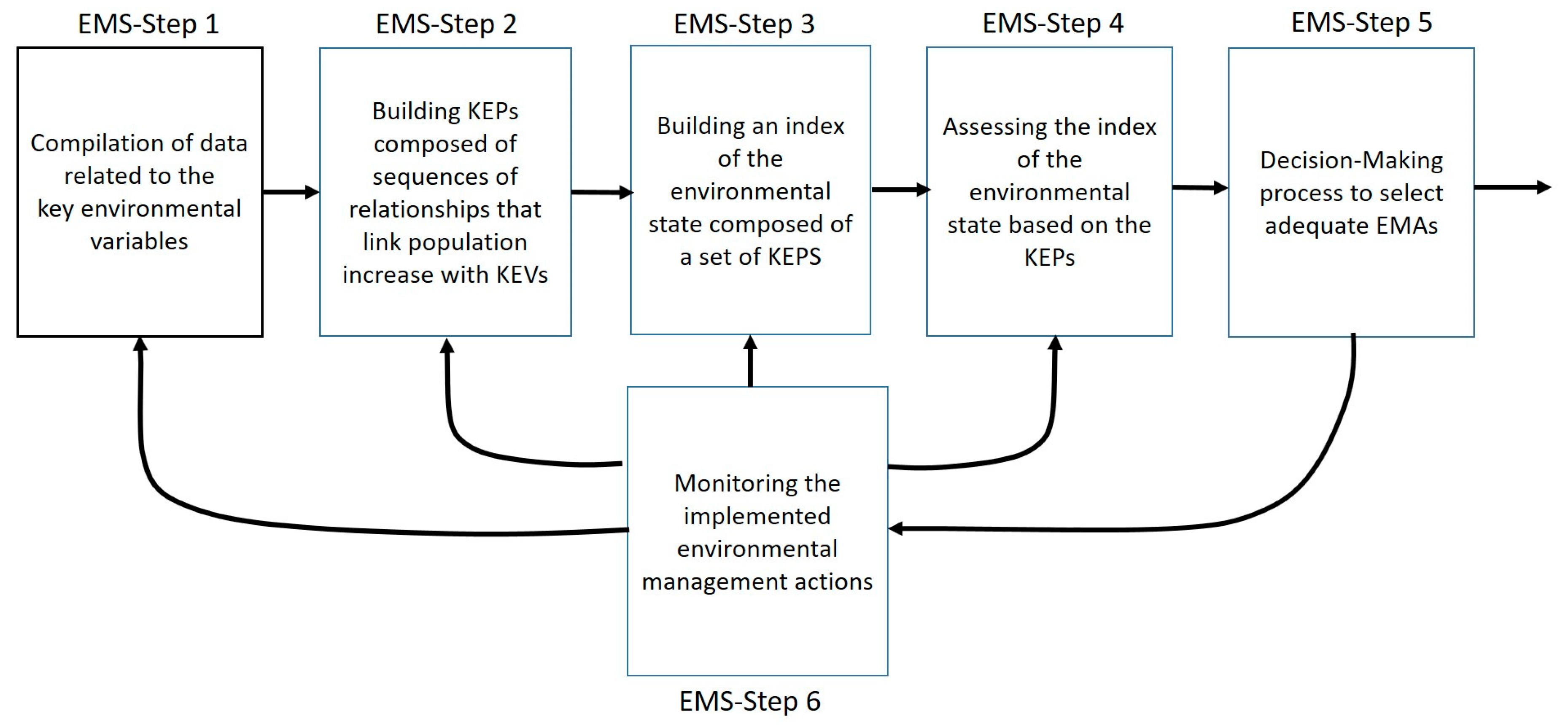
2.1.3. Integration of the CBR–AHP Hybrid Method into the EMS

The proposed method is part of the processes that take place within an EMS. This method is focused on the decision-making process of the EMS. In order to facilitate the understanding of the processes involved in the EMS, we will give a brief description of them by highlighting the importance of the role of the proposed method within the decision-making process. A simplified version of the EMS, represented by a block diagram, is used to describe the processes involved in the EMS (see Figure 1).
Due to the fact that the EMS was already reported [45], it is included in this section of materials. In contrast, the decision-making process, which is situated in the EMS-Step 5 of the EMS, will be described in the methods section, because it is the main proposal of this work.
We will briefly describe the processes taking place within the EMS, which is composed of 6 steps. The EMS-Step 1, EM-Step 2, EM-Step 3, and EMS-Step 4 are already developed and reported [44]. The EM-Step 5 is presented in this work. Due to the fact that the EM-Step 6 is currently under development, it is only mentioned but not analyzed. Figure 1 (below) depicts the steps of the EMS.
A brief description of the EMS. Our main objective was to study the effects of the population increase, playing the role of a driving-force variable, on pressure variables, which affect the state of the environmental quality and cause impacts on different issues related to the environment. Based on assessments of the environmental state, a set of EMAs are proposed. The selection of adequate EMAs becomes a challenge for decision makers to support a sustainable performance of the EMS.
On the processes taking place within the EMS. Based on Figure 1, the EMS starts with the compilation of data related, with 9 variables from which we build a set of causal relationships (EMS-Step 1), which are mainly associated with socioeconomic and environmental aspects. In the EMS-Step 2, a set of key environmental pathways (KEPs) linking the population increase with KEVs are built and aggregate to build an environmental state index in the EMS-Step 3. Thus, KEPs are composed of a sequence of cause–effect relationships between drivers and pressure variables. Each KEP is associated with one KEV, namely CO2 emissions, solid waste, water availability, loss of vegetation cover, and air quality. In the EMS-Step 4, the assessment of risky trends of KEPs is carried out, which will be used as input data to EMS-Step 5, where the decision-making process to select adequate EMAs takes place. Finally, the implementation of the adequately selected EMAs should be monitored to assess their performance, which takes place in EMS-Step 6.

2.1.4. Set of KEPs

The set of KEPs is described in Table 2. A main characteristic of these KEPs is that they link the population node with the nodes representing the KEVs, and all of them converge into the global environmental state (GES) node. As we can see, a GES index or aggregate indicator was built, because the five KEPs converge into the GES node.

2.1.5. A Set of EMAs to Improve the Environmental State

Appendix B shows a set of EMAs. One or several of these EMAs represent alternatives to reduce the trends of the KEPs and, consequently, of the GES.

2.1.6. The OECD-Outlook to 2030

The OECD has proposed an Environmental Outlook to 2030 that depicts a set of favorable and unfavorable environmental scenarios associated with semaphore lights, as follows (text reproduced from [44]): “Green light = environmental issues which are being well managed, or for which there have been significant improvements in management in recent years but for which countries should remain vigilant; Yellow light = environmental issues which remain a challenge but for which management is improving, or for which current state is uncertain, or which have been well managed in the past but are less so now. Red light = environmental issues which are not well managed, are in bad or worsening state, and require urgent attention.”
These scenarios could be reached from the current state, depending on the implementation or non-implementation of EMAs.

2.2. Methods

The methods shown in this work are related to the decision-making process taking place in Step 5 of the EMS, which is shown in Figure 1.
Figure 2 depicts the steps of the decision-making process aimed at selecting a set of adequate EMAs, given a set of risky trends of the KEPs. The description of the current situation takes place in DM-Step 1 (DM stands for decision-making). The current situation is composed of trend values of KEPs. These KEP values are the input of one of the two modules of the DM-Step 2, which is in charge of providing an order of priority of KEPs by applying the AHP method. This method also checks the consistency of the provided order. In DM-Step 3, a set of weighted KEPs representing the current situation is the input data of the similarity calculations to retrieve similar cases stored in the MC. The output of the DM-Step 3 represents a set of retrieved cases whose situations are the most similar to the current situations. This set of retrieved cases is provided to the adaptation mechanism. In DW-Step 4, when two or more than two EMAs are proposed as candidates for the solution, the EMAs are ordered by priority using the AHP method, which also checks the consistency of the order of priority. The output of the DM-Step 4 provides the selected EMAs by order of priority to decision makers. Finally, new situations and/or solutions, as well as modified situations and/or solutions, will be stored in the MC in the refinement process that takes place in DM-Step 5.
The framework of the CBR method of this paper has the common components of the traditional frameworks found in [31,32,33,34,35].
The next sections deal with the methods and concepts associated with the CBR–AHP hybrid method proposed in this work by following the steps depicted in Figure 2.

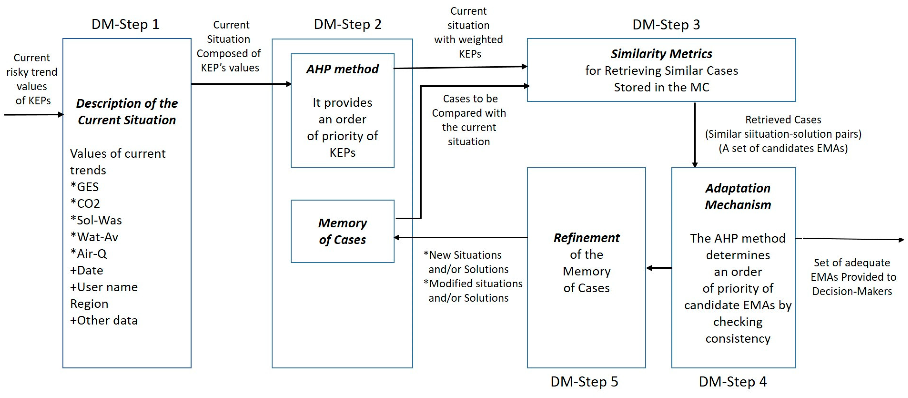
2.2.1. DM-Step 1: Description of the Current Situation

The behavior of the trend values of KEVs over time is due to a sequence of cause–effect relationships between drivers and stressors that damage the environmental state. Such sequences are represented by KEPs, which are combined to build the GES index. This is the reason why we use trend values of KEPs in the construction of situation–solution pairs or cases to be stored in the MC. Therefore, the current situation is described in terms of current trend values of KEPs. In addition, through the use of KEPs, we are able to identify those relationships that are causing the most, or the least, damage to the GES. One KEP is always associated with one KEV.
These current trend values can be expressed in angular or normalized values as shown below.
State:
  • Path_CO2: Angular value/Normalized value
  • Path_Sol-Was: Angular value/Normalized value
  • Path_Wat-Av: Angular value/Normalized value
  • Path_LVC: Angular value/Normalized value
  • Path_Air-Q: Angular value/Normalized value
  • GES: Angular value/Normalized value

2.2.2. DM-Step 2: The MC and the Order of Priority of KEPs

Several considerations concerning the construction of the MC were taken into account. A set of KEPs associated with five KEVs were defined; we assessed the trend values of each KEP with risk values belonging to a range expressed in three different terms: tangent values (0, ∞); angular values (0°, 90°); and normalized values (0, 1), where 0 or 0° represents the minimum risk and ∞, 90°, and 1 represent the maximum. Five regions at risk were determined where a given trend value could fall inside; these regions at risk will be composed of a finite number of predefined situations, along with their solutions, which are composed of a set of EMAs.
A situation in the MC will be mainly composed of six values, corresponding to the five KEPs and the GES value. Meanwhile, the solution contains EMAs aimed at reducing the trends of the KEPs associated with the highest-risk trend values. The MC used in this work is shown in Appendix C, which is composed of 243 cases or situation–solutions pairs.

Method to Define the Number of Potential Cases to Be Stored in the MC

Considering that the trend value of a KEP can fall inside five potential zones at risk, as described in Table 3, the total number of situations would be Rn, where R is the number of KEPs and n is the number of regions at risk. Hence, R = 5 and n = 5, thus 55 = 3125 potential situations by considering only one value for each KEP. This value will be represented by the centroid value of the regions at risk, which are expressed in angular or normalized values in Table 3. The centroids are also shown in the third and fifth columns of Table 3.
Thus, each KEP could have five centroid values, one for each region at risk. The main reason why the centroid of each region at risk is chosen is that we need a reference of each region at risk to initiate the search for a situation stored in the MC similar to the current situation.
As the number of regions at risk rises, the number of potential solutions rises. And as the number of KEPs increases, the number of potential solutions increases, as well. For example, if we suppose that the number of regions at risk increases up to eight zones and the number of KEPs up to six, then the result would be 68 = 1,679,616 potential situations. Thus, an exponential increase is expected as both variables increase. As we can see, this number of potential situations is not easy to handle in practical terms.

A Pruning Method to Reduce the Number of Potential Cases to Be Stored in the MC

A practical and representative number of situation–solution pairs (cases) should be stored in the MC. As explained before, the number of potential situations by considering one reference value (the centroid of the regions at risk) for each one of the five regions at risk and five KEPs would yield 55 = 3125 potential situations. On the other hand, the solution will be composed of a set of EMAs to be proposed to users. If we consider five EMAs (see Appendix B) for each KEP, then the potential solutions will be 55 = 3125 potential solutions. Therefore, the total number of potential situation-–solution pairs (cases) would be 3125 × 3125, and then the total of potential situation–solution pairs (cases) would be 9,765,625. This number of cases stored in the MC would be very hard to handle from a practical point of view. However, we can reduce this complexity by considering practical measures. For example, the current situations falling inside the regions at very low and low risk are not candidates to implement EMAs because these regions are not at risk at all. Thus, the number of potential situations that are candidates to apply EMAs would be reduced to 35 = 243, which corresponds to the regions at medium, high, and very high risk for the five KEPs. We can verify that 243 situations represent 7.77% of the total of 3125 potential situations, if the five regions at risk were considered. At the same time, we could consider two of the EMAs for each potential situation, which yields 25 = 32 potential solutions for each potential situation. Finally, after applying these pruning measures, the total of potential situation–solution pairs (cases) would yield 243 × 32 = 7776. This number of cases is easier to handle.
Another criterion to reduce the number of cases is related to the current situations that have one, or more than one, KEP whose current trend is located in the region at high risk or in the region at very high risk. We will give priority to those current values of the KEPs that fall either inside the regions at high or very high risk. More precisely, with normalized values ≥0.777 or ≥0.944. Derived from this consideration and based on 243 cases derived from the combination 35 = 243 mentioned before, we have classified the situations stored in the MC in accordance with their associated EMAs as follows: 85 with three EMAs, 76 with four EMAs, 40 with two EMAs, 31 with five EMAs, and 11 with one EMA.

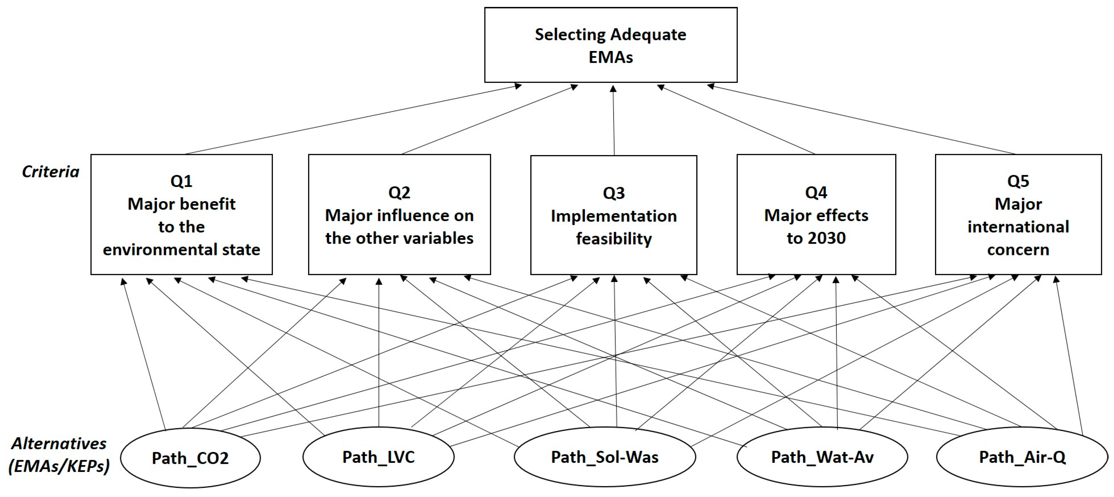
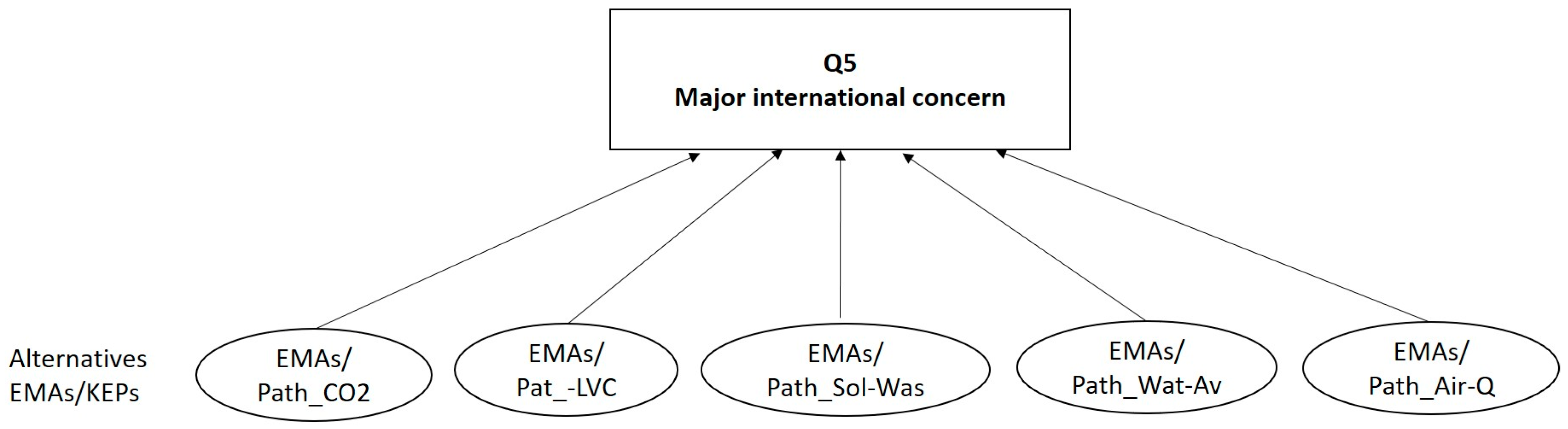
The AHP Method to Determine the Order of Importance Given to the Questions

The calculation of similarity measure requires weighting KEPs for the simple reason that they are not of the same nature. The purpose of weighting KEPs is to assign them a level of relevance within a particular context, which is composed of specific socioeconomic and sociopolitical factors, technical capacities to implement the EMAs, and the capacity of each variable to affect the state of other variables. The fact of assigning weights to a set of KEPs requires verifying consistency of the order of priority. The consistency checking will be carried out by the AHP method.
The methods to assign weights to KEPs need reliable information and knowledge in order to be valuable and usable. In the domain of environmental problems, the direct intervention of experts is more reliable [55]. Such information and knowledge can be elicited through the direct intervention of experts. Knowledge elicitation is the process of collecting information from human knowledge that is thought to be relevant to that knowledge [56]. In direct elicitation methods, the domain expert is questioned to obtain information, which has to be easily expressed by the expert. A direct method is the application of a questionnaire [57,58,59,60].
We consulted a group of experts to determine an order of preference to be assigned to the KEPs associated with EMAs and to the issues contained in the questions. The experts belong to different areas, namely climate change, water, solid waste, biodiversity, and air quality. For each question, the expert should know the real context of the region. Table 4 shows the questions applied to a group of experts.
The process to weight the KEPs is composed of three steps: (1) We have prepared a questionnaire designed to define the criteria from which the order of priority of KEPs is determined; (2) we have defined an order of preference both for the questions and for the KEPs; and (3) the AHP method was applied to verify the consistency of the order of preference given to criteria and to KEPs.
The order of preference, for five variables can be expressed as follows: X1 > X2 > X3 > X4 > X5. Eventually, the order of preference between two variables can be defined by “equal”; for example, X3 = X4, which can be read as X3 is equally preferred to X4. A scale of pairwise comparison is shown in [42], with the following order of preference: extremely preferred (9), very strongly to extremely (8), very strongly preferred (7), strongly to very strongly (6), strongly preferred (5), moderately to strongly (4), moderately preferred (3), equally to moderately (2), and equally preferred (1).
Table 5 shows two important averages: the points average obtained by KEPs and the points average obtained related to the five questions, both derived from the opinions of the experts. These averages will provide us with an estimation of the order of preference both for the KEPs and for the questions. The estimation of the order of preference for the questions is the following: Q5 > Q2 > Q1 > Q3 > Q4. Meanwhile, the estimation of the order of preference given to KEPs is the following: Path_LVC > Path_Wat-Av > Path_Sol-Was > Path_CO2 > Path_Air-Q. The AHP method will be used to confirm the order of preference for both the questions and the alternatives represented by KEPS associated to EMAs by checking the consistency ratio. Figure 3 shows the hierarchy to be analyzed, which shows at the first level the “Selecting Adequate EMAs” node that represents the goal to be reached, the criteria at the second level, and the alternatives at the third level. The criteria are derived from the questions shown in Table 4; meanwhile, the alternatives represent the EMAs/KEPs.
The AHP method applied to determine the order of importance given to the questions is shown below. The criteria comparison matrix (Matrix A) to determine the order of importance of the questions is shown below.
Matrix A:
QsQ1Q2Q3Q4Q5
Q111/3351/5
Q231571/3
Q31/31/5131/7
Q41/51/71/311/9
Q553791.0
Sum of Columns9.5334.67516.333251.786
The normalized column sums of the matrix A are shown below. The Eigen Vector is shown in column 7, which is determined by the average of each row.
QsQ1Q2Q3Q4Q5Eigen Vector (x) or Criteria Weights
Q10.1050.0710.1840.2000.1120.134
Q20.3140.2140.3060.2800.1860.260
Q30.0350.0430.0610.1200.0810.068
Q40.0210.0300.0200.0400.0640.035
Q50.5240.6410.4290.3600.5560.502
Sum of Columns111111
As shown by the Eigen Vector or criteria weights, the criterion described by Q5 is the most important one. It deals with the key environmental variable that represents the major international concern.
The next step is to check for consistency. For example, it should meet the transitivity rule as follows: If criterion A is preferred to criterion B, and B is preferred to C, then A is preferred to C. If the consistency ratio is CR ≤ 0.1, it indicates sufficient consistency for decision.
[Ax]·[x]−1 is called the consistency vector. λmax (the Eigen Value) determines the average of the elements of the consistency vector, which is defined as follows: λmax = average[Ax]·[x]−1. The consistency vector represented horizontally is the following:
[Ax] = [0.134 0.260 0.068 0.035 0.502]
and the Eigen value λmax is:
λmax = average (0.699/0.134 + 1.414/0.260 + 0.341/0.068 + 0.177/0.035 + 2.743/0.502)
λmax = 5.238
The consistency index (CI) is calculated as follows: CI = (λmax − n)/(n − 1) = (5.238 − 5)/(5 − 1) = (0.238/4) = 0.0595, where n = 5, which represents the number of the criteria. We calculate CR, the consistency ratio, which is defined by the following expression: CR = CI/RI, where RI is the random index.
The value of the RI depends on the number of alternatives (n), as shown below. As mentioned in Section 1.2, based on the Saaty scale, the RI value depends on the number of entities of criteria and alternatives represented by n [42]. In our case n = 5, thus, the RI value is 1.1.
n1234567
RI000.520.881.11.251.35
Finally, the consistency ratio is CR = CI/RI = 0.053/1.1 = 0.048. It indicates sufficient consistency for decision because CR < 0.1.

The AHP Method to Determine the Order of Priority of the Alternatives (KEPs)

Thus, we have to consider the five alternatives representing the KEPs for each of the criteria based on Q1, Q2, Q3, Q4, and Q5, as shown in Figure 3, Section 2.2.2. For lack of space, we determine only the weights assigned to alternatives linked to the criterion Q5, as shown in Figure 4. As mentioned before, the estimation of the order of preference given to KEPs associated with their EMAs is the following: Path_LVC > Path_Wat-Av > Path_Sol-Was > Path_CO2 > Path_Air-Q.
Matrix A is shown below:
EMAs Related to KEPsPath_CO2Path_LVCPath_Sol-WasPath_Wat-AvPath_Air-Q
Path_CO211/71/31/53
Path_LVC71539
Path_Sol-Was31/511/35
Path_Wat-Av51/3317
Path_Air-Q1/31/91/51/71
Sums of columns16.3331.7869.5334.67525
Matrix A with normalized values and the priority or Eigen Vector.
EMAs Related to KEPsPath_CO2Path_LVCPath_Sol-WasPath_Wat-AvPath_Air-QPriority or Eigen Vector
Path_CO20.0610.0790.0350.0430.120.068
Path_LVC0.4280.5590.5240.6420.360.503
Path_Sol-Was0.1830.1120.1050.0710.200.134
Path_Wat-Av0.3060.1860.3150.2130.280.260
Path_Air-Q0.0200.0620.0200.0300.0400.034
Sums of columns11111
We recall that the following results are related to alternatives linked to Question 5. We can verify from the Eigen Vector that Path_LVC was assigned with the highest weight value (0.503). The second place is occupied by Path_Wat-Av, Path_Sol-Was is in third place, Path_CO2 is in fourth place, and Path_Air-Q is in fifth place.
The λmax (the Eigen value) in this case is the one shown below:
λmax = average [0.337/0.068 + 2.735/0.503 + 0.696/0.134 + 1.407/0.26 + 0.177/0.034] = 5.236
The consistency ratio is the following:
consistency index: CI = (λmax − n)/(n − 1) = (5.236 − 5)/(5 − 1) = (0.236/4) = 0.059
consistency ratio = CR = CI/RI = 0.059/1.1 = 0.053, where RI = 1.1, from the table shown below:
n1234567
RI000.520.881.11.251.35
Finally, CR ≤ 0.1, which indicates sufficient consistency for decision.

2.2.3. DM-Step 3: The Similarity Measure Method to Retrieve Similar Situations from the MC

A similarity method is used to retrieve those situations stored in the MC similar to the current one. The similarity measure uses Euclidian metrics, whereby the math function to determine the similarity value is represented by Equation (1); it calculates similarity measures without weights [61].
S ( x i , y i ) = [ i = 1 n | ( x i y i ) 2 | ]
The Euclidian distance when weights are assigned to all the attributes is shown in Equation (2) [55]:
S ( x i , y i ) = [ ( i = 1 n w i r | ( x i y i ) r | ) / ( i = 1 n w i r ) ] 1 / r
where x = [x1, x2, …… xn] represents the array of attributes belonging to the current situation; y = [y1, y2, ……. yn] is the array of attributes representing any situation stored in the memory of cases; i is an integer number from 1 to n; and n is an integer representing the number of attributes associated with each situation for both the current situation and the situations stored in the memory of cases. The attributes are related to KEPs. The GES does not belong to the attributes to be compared to calculate the similarity between two situations. The GES value is a very good guide for finding situations belonging to the MC similar to the current one. The situations stored in the MC similar to the current one are in the neighborhood of its GES value.
In Equation (2), w i r represents the weight value to be assigned to the n attributes, and r takes the value of 2. We have five variables to be weighted with values between 0 and 1. For obvious reasons, a variable cannot be assigned with the value of “0”. Several sets of five weights can be defined; the following are examples: [0.2, 0.3, 0.4, 0.5, 0.6] or [0.3, 0.4, 0.5, 0.6, 0.7] or [0.4, 0.5, 0.6, 0.7, 0.8] or [0.5, 0.6, 0.7, 0.8, 0.9] or [0.6, 0.7, 0.8, 0.9, 1] or [0.2, 0.4, 0.6, 0.8, 1]. We selected the range [0.5 to 0.9], but we could also select other ranges. The only condition is that the most significant weight should be the one closer to 0 and the less significant the one closer or equal to 1.
We show below an example of the similarity between a situation stored in the MC and a current situation. The similarity calculation will be performed based on the following considerations: w 1 2 is the weight assigned to the term |(x1y1)|2, which represents the difference between the value of the variable CO2 corresponding to the current situation (x1) and the value of the variable CO2 (y1) that corresponds to a situation stored in the MC. Following a similar procedure, w 2 2 corresponds to the variable solid waste, w 3 2 corresponds to the variable water, w 4 2 corresponds to the variable LVC, and w 5 2 corresponds to the variable Air-Q.
For this example, the weights assigned to environmental variables are 0.7 for CO2; 0.6 for waste; 0.9 for water; 0.5 for LVC; 0.8 for air quality. As we can see, the highest weight value (0.5) was assigned to the LVC variable. We use Equation (2), shown in Section 2.2.3, for the calculation of similarity measure, using the weight assigned to the involved variables.
The current situation is described in Table 6, using normalized and angular values. As we can see, the GES is situated in the region at high risk due to the effects of the trend values associated with CO2, waste, and LVC. The most similar situations stored in the MC with this current situation by applying weights are also shown in Table 6.

2.2.4. DM-Step 4: The Adaptation Mechanism

The Adaptation Mechanism. The role of the adaptation mechanism is to build a set of EMAs by combining the EMAs provided by the retrieving process of the most similar cases stored in the MC. When a current situation is presented, it is compared to situations stored in the MC, using the similarity measure method described in Section 2.2.3. This mechanism will allow users to recover a set of the most similar cases to the current situation. The literature recommends recovering not only the most similar one but a set of those close to—or in the neighborhood of—the most similar one. Having several similar cases will facilitate the adaptation mechanism to obtain the final solution by combining the recovered cases.
Based on the example shown in Section 2.2.3, the solutions associated with the most similar situations stored in the MC and the fact that the key environmental variables, LVC, Waste, and CO2, were weighted with the highest values, three of these five solutions propose a combination of EMAs related to the three most weighted variables. The most similar solutions contain the EMAs related to LVC, Waste, and CO2: S81, S113, and S84.
The application of the AHP method to confirm the order of priority from a set of EMAs associated with the key environmental variables, LVC, Waste, and CO2, should be supported by the order of priority of these variables, which was already determined in Section 2.2.2. This order of priority was LVC > Wat-Av > Sol-Was > CO2 > Air-Q. Derived from this priority, the priority that corresponds to this example is LVC > Sol-Was > CO2. The consistency of order of this priority was already checked in this same (Section 2.2.2).

2.2.5. DM-Step 5: The Refinement Process

The refinement process takes place in one of the following cases:
(1)
If no similar situation to the current situation is found in the MC, then it is incorporated as a new situation in the MC;
(2)
If the adapted solution required more than five stored situations and their solutions need to be defined;
(3)
If the adapted solution is not yet included in the MC.
For example, the current situation treated as an example in the preceding section was specified by the following normalized values of environmental variables:
CO2WasteWaterLVCAir-QGESRegion at Risk
Current Situation0.7200.830.6300.8820.5000.7124high-risk
This situation was not part of the initial MC; thus, it is a serious candidate to enrich or refine the MC.

3. Analysis and Discussion of Results

In this work, the trend of the current environmental state is composed of trends of five KEPs related to the following KEVs: CO2 emissions, air quality, loss of vegetation cover, water availability, and solid waste. The combination or aggregation of these five KEPs will result in a trend of the GES. Thus, the risky trends of five KEPs represent a problem that needs solving.
Meanwhile, the solution consists of proposing implementable EMAs aimed at reducing those trends that put at risk the environmental quality of a region under study. These KEVs were chosen because of two main reasons: (1) They are related to the OECD’s Outlook to 2030 that aims to manage the state of the environmental quality [44]; and (2) our interest is to make this study with real information available from official sources (national and/or international), during a considerable period of time (at least 10 years). Other important variables, such as industrial emissions or non-solid waste, among others, were not considered, due to lack of information.
The discussion of results will follow the steps of the decision-making process shown in Figure 2.

3.1. On the DM-Step 1: Description of the Current Situation

The current situation could be defined by a set of current trend values of KEPs that compose the environmental state. However, the assessments of the trends related to isolated variables over time, whose combination or aggregation represent the global environmental state, results in an incorrect judgement. Instead, the combination of a set of sequences of cause–effect relationships, named KEPs, between drivers and stressors should be considered to represent the global environmental state. In addition, KEPs are able to identify what cause–effect relationships are impacting the environmental state the most or the least.

3.2. On the DM-Step 2: Memory of Cases and Priority of KEPs

3.2.1. Analysis of Cases to Be Stored in the MC

The following considerations to build the predefined MC were taken into account: (a) Any current situation should always find a set of similar situations from the MC and their corresponding solutions. (b) The definition of cases is related to the KEPs because they link drivers with stressors that exert effects on the environmental state. Thus, the cases can be analyzed not only by the values of isolated key environmental variables, but also by the relationships that have effects on them.
The initial set of cases to be stored in the MC always represents a challenge because we have to avoid a huge number of cases or situation–solution pairs. However, it should be representative enough for the initial sessions to retrieve similar cases to current situations. Based on practical reasons, we have considered only three regions at risk (medium, high, and very high) and two EMAs per environmental pathway, thus obtaining 243 potential situations and 32 potential solutions.
We can estimate that, as the number of EMA candidates increases, conflicting situations can occur at the moment of choosing one EMA over another, especially when the EMAs to be selected from are more than 2.

3.2.2. Analysis of the Method to Assign Weights to KEPs

We used a direct elicitation method [57,58,59,60] to obtain the information related to determine preferences assigned to KEPs through a questionnaire depicted in Table 4. The experts who responded to the questionnaire belong to domains related to climate change, biodiversity, water, solid waste, and air pollution. However, the diversity of domains of expertise can bring about conflicts due to the different points of view of experts, thus putting at risk the assignment of weights based on objective judgements. One way of reducing such conflicts is gathering experts with a very good level of knowledge of the environmental problems related to the region under study. This condition helps reduce wrong judgments about the needs and limitations of the region under study.
For example, based on the questionnaire, the preference given to the KEPs by the experts of the region was as follows (the position obtained by each KEP is written in parentheses): Path_LVC (1), Path_Wat-Av (2), Path_Sol-Was (3), Path_CO2 (4), and Path_Air-Q (5). However, this order may certainly change in other regions, because the application of judgments depends on the environmental needs, sociopolitical and socioeconomic factors, and technological skills and/or limitations to implement EMAs, which are surely different for different regions. However, it is worth analyzing the order of preference based on each of the questions, whose results are shown in Table 5.
The questions played an important role in determining the criteria and an order of preference of alternatives represented by KEPs associated with their corresponding EMAs. The first four questions have a similar order of preference, so we can say that three variables dominant over the preference of experts: LVC, Wat-Av, and Sol-Was. In these first four questions, LVC always takes the first place. Meanwhile, Wat-Av and Sol-Was exchange the second and third place with each other. We can see that CO2 occupies the four place three times out of five. And Air-Q always occupies the last place.
In conclusion, based on the opinions of experts, the EMAs’ related to reducing the LVC will provide a major benefit to the current environmental quality. It exerts negative impacts on CO2 emissions and water scarcity; however, LVC suffers effects from water scarcity, waste, CO2 emissions, forest fires, and the construction of transportation roads. Even though the development of new urban areas and industrial parks, as well as changes in land use, affect the LVC, they were not included in this study because of lack of information. Due to the fact that LVC, water availability, and solid waste are quite related, we show a brief analysis of these three variables and some important problems associated with them.
On the LVC: The Payment for Environmental Services (PES) program was introduced in Mexico in 2003 as a response to deforestation rates, aquifer overexploitation, and high poverty rates in rural areas. The PES program has had a low impact due to several problems: a wrong definition of eligibility zones; the criteria to select plots needs to be redefined [62]; the decision makers have different interests because they belong to different organizations and institutions; the payments for all forests are flat, which is egalitarian, but highly inefficient [63]; and the lack of monitoring the performance of the PES program, among others [64].
On water availability. Some of the problems related to water in the state of Morelos are bad maintenance of water wells; contamination of ravines and rivers; overexploitation of aquifers, which deteriorates water quality due to saline intrusion and fossil water migration concentrated naturally; water pollution due to the discharge of domestic, industrial, agricultural, and mining residues; and inadequate water distribution systems requiring constant monitoring to detect leaks and repair obsolete water distribution networks. The unavailability of water, the inefficient use of water in agriculture and urban zones, and the lack of use of rainwater are other important issues related to this problem [65]. These problems require long-term integral management planning at a national level, which unfortunately does not exist, so far [66].
On solid waste. As population increases, waste generation also increases due to human activities, thus bringing about a decrease in water supply and water quality. An important issue in municipal solid waste management is the construction of adequate landfills; otherwise; the waste produces wastewater, which in turn pollutes the soil and surface water. In addition, high concentrations of PM10, Mn, and Ni were found in air samples, which exceeded the permissible limits [67]. Thus, sanitary landfills are required and should be located in adequate places to avoid the contamination of groundwater. Water resources would benefit from adequate studies focused on the location of potential landfills. We can confirm that relevant cause–effect relationships take place between solid waste generation and the availability and quality of water [68].
The order given by experts to Question 4 was similar to the order given to Questions 1, 2, and 3. This order is consistent with the order given to the previous questions, as long as it is based on a regional perspective. In conclusion, we consider the reason the experts chose the LVC, water, and waste as those with the highest weights is because of their strong relationships, as described above.
Question 5 is related to a key environmental variable that represents the most international concern. Even though CO2 emissions are of high current international concern, water availability occupied first place in this question. We recall that CO2 emissions are the grounds for international concern, resulting from the Paris climate agreement (COP 21, 2015), which sought to curb greenhouse gas (GHG) emissions and limit global temperature increase to between 1.5 and 2 °C [69]. In addition, the Special Report on Global Warming of 1.5 °C by the IPCC in the Republic of Korea [70] called for limiting global warming to 1.5 °C compared to 2.0 °C. As already discussed, at a regional level, in Mexico, water availability represents such an important concern for local communities that it has taken the place of the worry about CO2 emissions as the most important environmental concern. Certainly, CO2 emissions represent the most international concern in terms of developed countries, mainly because they have a high level of environmental education and considerable economic resources oriented to finding solutions to reduce CO2 emissions. Example include those countries belonging to the European Union. Instead, for developing countries, for example, in Latin America and Africa, the major concern is, without any doubt, water availability.

3.3. Analysis Related to the Adaptation Mechanism

As already mentioned, as the number of EMAs provided by the CBR–AHP method to decision makers increases, conflicting situations can occur at the moment of choosing one EMA over another. When high trend values of 3, 4, or 5 KEPs fall inside the regions at high or very high risk, more than two EMAs related to KEPs are needed to be implemented. In such cases, conflicting situations can occur due to the fact that some EMAs could be more important for certain decision makers than for others. We have already analyzed that, in such cases, an order of priority based on the assigned weights given to KEPs helps considerably to solve this conflicting situation.
We illustrate this aspect with the example treated in Section 2.2.3 and 2.2.4, where four trend values of the KEPs belonging to the current situation fall inside the region of high risk (two KEPs) and inside the region of very high risk (two KEPs). The GES value falls inside the region of high risk. The current situation is expressed in terms of normalized values as follows: CO2 (0.720); waste (0.830); water (0.630); LVC (0.882); and air quality (0.500). Meanwhile, the weights assigned to the KEPs are 0.7 for CO2; 0.6 for waste; 0.9 for water; 0.5 for LVC; and 0.8 for air quality. The highest weight value was assigned to the LVC variable. The similar situations stored in the MC and their corresponding solutions were the following: S81 (1)/0.0628/LVC-CO2-Waste (it is read as follows: the situation 81 was the most similar to the current situation, whose similarity value was 0.0628. The EMAs associated with S81 are LVC/CO2/Waste. Based on this format the next similar situations have the following data: S50(2)/0.0682/CO2-Waste-Water; S113(3)/0.0734/Waste-LVC-CO2; S84(4)/0.0780/Waste-LVC-CO2; and S29(5)/0.0925/LVC-Waste.
We can conclude from these results that the highest weight value was assigned to LVC (0.5), followed by waste (0.6) and CO2 (0.7), and three out of five similar situations are composed of the same EMAs (LVC/Waste/CO2), which are proposed as EMAs to decision makers. This definitely simplifies the process of selecting EMAs. However, a problem remains to be solved: Which is the order of importance of these three EMAs? As we have shown, the CBR–AHP hybrid method proposed in this work solved this problem. The use of the AHP method provided decision makers with an order of importance of the KEPs associated with their EMAs by checking the consistency of the provided order to ensure an adequate selection of EMAs.
It is important to point out that the adaptation mechanism takes into consideration several factors to obtain the final solution. These factors can be derived from different causes related to regions where the EMAs would be implemented. These causes can involve socioeconomic, sociopolitical, and/or technical aspects. Among these aspects, we can mention the following: (1) the priority assigned to KEPs (e.g., the problems associated with solid waste could be the most important to be solved for a given region, but, for other regions, the most important variable could be a different environmental variable); (2) meeting the commitments related to international agreements to address the problem of climate change (e.g., based on COP-21, the reduction of CO2 emissions is the priority to avoid increasing temperatures beyond 2 °C for 2030); and (3) the technical feasibility to implement a given management action in a given region (e.g., a region may or may not dispose of instruments and professionally trained people to monitor the air quality). In addition, due to conflicting situations between opposing political parties, the agreements to support the generation of public policies aimed at facing certain priority environmental problems may not be concluded positively, thus delaying an urgent decision.
The CBR–AHP method integrated into the EMS has provided promising results through its units, such as the memory of cases, the method for weighting the KEPs, the process to retrieve similar cases from the MC, and the adaptation mechanism. Therefore, we consider that the integration of the CBR–AHP method into the environmental management system is a feasible proposal that is capable of providing valuable support to the decision-making process for the selection of appropriate EMAs aimed at improving the environmental state of a region.

4. Conclusions

The selection of a set of adequate EMAs to reduce the risky trends of the current environmental state of a region represents an important decision-making challenge. In addition, the selection of a set of inadequate EMAs already implemented put at risk a sustainable performance of an EMS. Such selection becomes more critical when decision makers should assign an order of priority to several candidate EMAs. In order to address this problem, we have proposed the integration of the CBR and AHP methods to select a set of adequate EMAs, thus supporting the sustainable performance of the EMS.
We have argued that the interactions—represented by cause–affect relationships in this work—between the involved variables that affect the environment make the complex task of selecting a suitable set of EMAs to improve the environmental-state quality difficult. We have also emphasized that the knowledge of the relationships between drivers and stressors that exert effects on the environmental state is basic to understanding important processes taking place in the environment which, in turn, will allow us to assess the environmental state to support decision makers in the selection of more-adequate EMAs.
The selection of a set of adequate EMAs should satisfy relevant aspects related to certain criteria determined by experts, who should know very well the environmental context of the region under study. The alternatives represented by EMAs should satisfy the criteria for selection, the set of EMAs should be ordered by priorities by formally checking the consistency of the given order, and the assessments of the current environmental state should reflect a general environmental context, instead of partial views associated with isolated environmental variables.
We have found that selection criteria based only on the assessments of current values of independent variables is not significant enough to reflect an acceptable environmental context. Therefore, we have proposed assessments of KEPs, because the behavior of the trend values of KEVs over time is due to a sequence of cause–effect relationships between drivers and stressors that converge into them. This is the reason why we use trend values of KEPs in the construction of situation–solution pairs or cases to be stored in the MC. In addition, through the use of KEPs, we are able to identify what relationships are causing the most, or the least, damage to the global environmental state. Finally, we point out that a KEP is always associated with a KEV.
Despite the advantages of the CBR method to reason about experiences or cases stored in the MC to solve new problems, this method is sensitive to inconsistent data without having the capacity to establish an order of priority of the involved variables, which is required in two important processes of the CBR method. The first process is during the calculation of the similarity value to retrieve similar cases to current situations. In this case, KEPs should be weighted to calculate the similarity value. The second process is during the adaptation process to obtain the solution by combining several candidate EMAs to build a solution. In this case, EMAs or alternatives should be weighted and ordered according to priority. Due to these disadvantages, the CBR method alone does not guarantee a selection of a set of adequate EMAs, and, consequently, the sustainable performance of the environmental management system can be affected. This disadvantage is an advantage in the AHP method. Thus, the advantages related to both methods were integrated to reinforce the decision-making process to select adequate EMAs.
The criteria and alternatives determined to select the EMAs to be implemented depend on the needs and the context of the region under study. This dependence is multifactorial, where socioeconomic, sociopolitical, and technological factors play a very important role in the decision-making processes. For example, the highest priorities assigned to EMAs may be water availability or loss of vegetation cover for certain regions of developing countries, such as Mexico. Instead, the reduction of CO2 emissions may be the highest priority for European countries. These aspects make the task of selecting adequate EMAs in the decision-making processes even more difficult. The hybrid method proposed aims to support decision makers in this complex task.
The results obtained provided significant insights into the capacity of the hybrid CBR–AHP method to support the decision-making process in the selection of adequate EMAs to reduce the risky trends of an environmental state in a region. Such results also suggest expanding the number of KEPs and EMAs to test the capacity of the CBR–AHP method in more-complex scenarios and verify the limits of the consistency-checking method as criteria and alternatives increase. For future study, this CBR method could be replicated and applied to other environmental issues. Another important issue for future study is to enrich the MC by providing cases with information related to hints about the effort necessary to implement EMAs and about the expected results derived from an eventual implementation of EMAs.

Author Contributions

Conceptualization, F.R.-Q. and H.S.-N.; data curation, E.T.-S., H.S.-N., and M.-L.C.-G.; formal analysis, F.R.-Q., E.T.-S., H.S.-N., and J.P.S.-H.; methodology, F.R.-Q., E.T.-S., H.S.-N., and J.P.S.-H.; validation, F.R.-Q. and M.-L.C.-G.; writing—original draft, F.R.-Q. and H.S.-N.; writing—review and editing, F.R.-Q.

Funding

This research was funded by the program CONACyT-FOMIX of the Mexican Government of the State of Morelos, under the project No. 189949.

Acknowledgments

We thank Rosalind Pearson Hedge for her comments and suggestions that improved our manuscript.

Conflicts of Interest

The authors declare no conflicts of interest.

Appendix A

In the table below, each year is associated with two lines: the upper line represents the average per year of each variable, and the lower one the percentage increase of each variable between the current year and the year 2000. The last line of this table shows the impacts on each variable during the period 2000–2010.
Table A1. The average per year and corresponding percentage increase of each involved variable from 2000 to 2010.
Year Pop (Inhabitants)CO2 (Gg)Trans-Ro (Km)FF (Ha)LVC (Ha)Wat-Av (m3/per)Trans-Ve (Vehicles)Sol-Was (tons)Air-Q
(PM2.5) (mass/m3)
2000Average1,555,2962816.220011290.42.818155,600459,0001.016 × 10−8
% Increase000000000
2001Average1,564,6272865.2202927201.52.818175,000472,000Lack of data
% Increase0.6001.7421.399 125 122.9012.4682.832Lack of data
2002Average1,574.0152974.88202969257.02.818187,500483,0001.009 × 10−8
% Increase1.2045.6341.399475184.29020.5015.2298.19
2003Average1,583,4593064.54202969329.72.713192,500493,0001.117 × 10−8
% Increase1.8118.8181.399475264.713.72623.7157.4079.95
2004Average1,592,9603231.57205869405.32.701200,000526,0001.078 × 10−8
% Increase2.4224.7492.848475348.344.08128.53514.5976.15
2005Average1,612,8993358.76208069476.12.746212,500538,0001.137 × 10−8
% Increase3.70419.2653.948475426.652.55536.56817.21111.99
2006Average1,645,1573530.68208069551.32.029250,000548,0001.184 × 10−8
% Increase5.77825.3703.948475509.8427.99960.66819.39016.58
2007Average1,678,0604552.01211272613.72.055270,000551,0001.285 × 10−8
% Increase7.89326.1275.547500578.8727.07673.52220.04426.49
2008Average1,711,6213652.88247775.5681.82.049290,000555,0001.187 × 10−8
% Increase10.05129.70923.788529.16654.2027.28986.37520.91516.86
2009Average1,745,8543784.18247777.5762.72.040310,000558,0001.049 × 10−8
% Increase12.25234.37123.788545.83743.6927.60899.22921.5693.31
2010Average1,777,2273859.22298678.5843.31.987340,000596,0001.063 × 10−8
% Increase14.26937.03649.325554.16832.8529.489118.50929.8474.66
Impacts: Percentage difference between 2010 and 2000The population increased 14,269%The CO2 emissions increased 37.036%The transport routes increased almost 50%The forest fires increased 554%The loss of vegetation cover increased 832%Water availability decreased almost 30%The number of vehicles increased 118.5%The solid waste increased almost 30%The PM2.5 increased almost 5%

Appendix B

Table A2. The Environmental Management Actions (EMAs) to Be Selected.
Key Environmental VariablesEnvironmental Management Actions
CO2 Emissions(1) A program of road re-engineering along with an interstate vehicle verification with mobility restrictions, mainly within metropolitan zones; (2) modernization of the vehicle fleet; (3) hybrid and electric vehicles; (4) the use of alternative fuels such as ethanol and biodiesel; (5) the reorganization of loading and passenger transportation.
Solid Waste(1) Construction of infrastructure for the separation, recycling, collection and disposal of waste; (2) construction of regional composting plants in areas of high organic waste generation and strategic areas for agriculture; (3) a formal inter-state program for the prevention and integral management of waste; (4) an ongoing awareness campaign for the reduction of the generation of solid waste.
Water Availability(1) Modern infrastructure for an efficient management and monitoring of continuous operation of the existing waste-water treatment plants; (2) modern hydraulic infrastructure that ensures the extraction, the supply and adequate use of the liquid for domestic purposes; (3) the reuse of treated water to reduce the consumption of water of first quality; (4) a program of capture and use of rainwater in priority areas.
Loss of Vegetation Cover(1) Protected natural areas; (2) payment of environmental services; (3) ecological zoning of the territory; (4) monitoring and control of forest fires; (5) reforestation.
Air Quality(1) Vehicle transport control; (2) forest fires control; (3) environmental education; (4) clean production; (5) avoiding burning the residues of the sugarcane crop by using them for fertilizer, biodigesters, and power generation, among others.

Appendix C

Table A3. The Memory of Cases (MC).
SituationsPath CO2Path WastePath WaterPath LVCPath Air-QGES (Norm)GES (ang)Regions at Risk of the GESSolutions
10.5550.555say 0.5550.5550.5550.55550midIt does not apply because the paths have the same value
20.5550.5550.5550.5550.7770.654midAir-Q
30.5550.5550.5550.7770.5550.654midLVC
40.5550.5550.7770.5550.5550.654midWater
50.5550.7770.5550.5550.5550.654midWaste
60.7770.5550.5550.5550.5550.654midCO2
70.5550.5550.5550.5550.9440.63357midAir-Q
80.5550.5550.5550.9440.5550.63357midLVC
90.5550.5550.9440.5550.5550.63357midWater
100.5550.9440.5550.5550.5550.63357midWaste
110.9440.5550.5550.5550.5550.63357midCO2
120.5550.5550.5550.7770.7770.64458midLVC/Air-Q
130.5550.5550.7770.5550.7770.64458midAir-Q/Water
140.5550.5550.7770.7770.5550.64458midLVC/Water
150.5550.7770.5550.5550.7770.64458midWaste/Air-Q
160.5550.7770.5550.7770.5550.64458midWaste/LVC
170.5550.7770.7770.5550.5550.64458midWaste/Water
180.7770.5550.5550.5550.7770.64458midCO2/Air-Q
190.7770.5550.5550.7770.5550.64458midCO2/LVC
200.7770.5550.7770.5550.5550.64458midCO2/Water
210.7770.7770.5550.5550.5550.64458midCO2/Waste
220.5550.5550.5550.7770.9440.677261highAir-Q/LVC
230.5550.5550.5550.9440.7770.677261highLVC/Air-Q
240.5550.5550.7770.5550.9440.677261highAir-Q/Water
250.5550.5550.7770.9440.5550.677261highLVC/Water
260.5550.5550.9440.5550.7770.677261highWater/Air-Q
270.5550.5550.9440.7770.5550.677261highWater/LVC
280.5550.7770.5550.5550.9440.677261highWaste/Air-Q
290.5550.7770.5550.9440.5550.677261highLVC/Waste
300.5550.7770.9440.5550.5550.677261highWater/Waste
310.5550.9440.5550.5550.7770.677261highWaste/Air-Q
320.5550.9440.5550.7770.5550.677261highWaste/LVC
330.5550.9440.7770.5550.5550.677261highWaste/Water
340.7770.5550.5550.5550.9440.677261highAir-Q/CO2
350.7770.5550.5550.9440.5550.677261highLVC/CO2
360.7770.5550.9440.5550.5550.677261highCO2/Water
370.7770.9440.5550.5550.5550.677261highWaste/CO2
380.9440.5550.5550.5550.7770.677261highCO2/Air-Q
390.9440.5550.5550.7770.5550.677261highCO2/Waste
400.9440.5550.7770.5550.5550.677261highCO2/Water
410.9440.7770.5550.5550.5550.677261highCO2/Waste
420.5550.5550.7770.7770.7770.688262highWater/LVC/Air-Q
430.5550.7770.5550.7770.7770.688262highWaste/LVC/Air-Q
440.5550.7770.7770.5550.7770.688262highWaste/Water/Air-Q
450.5550.7770.7770.7770.5550.688262highWaste/Water/LVC
460.7770.5550.5550.7770.7770.688262highCO2/LVC/Air-Q
470.7770.5550.7770.5550.7770.688262highCO2/Water/Air-Q
480.7770.5550.7770.7770.5550.688262highCO2/Water/LVC
490.7770.7770.5550.5550.7770.688262highCO2/Waste/Air-Q
500.7770.7770.5550.7770.5550.688262highCO2/Waste/Water
510.7770.7770.7770.5550.5550.688262highCO2/Waste/Water
520.5550.5550.5550.9440.9440.710664highLVC/Air-Q
530.5550.5550.9440.5550.9440.710664highWater/Air-Q
540.5550.5550.9440.9440.5550.710664highWater/LVC
550.5550.9440.5550.5550.9440.710664highWaste/LVC
560.5550.9440.5550.9440.5550.710664highWaste/LVC
570.5550.9440.9440.5550.5550.710664highWaste/Water
580.9440.5550.5550.5550.9440.710664highCO2/Air-Q
590.9440.5550.5550.9440.5550.710664highCO2/LVC
600.9440.5550.9440.5550.5550.710664highCO2/Water
610.9440.9440.5550.5550.5550.710664highCO2/Waste
620.5550.5550.7770.7770.9440.721665highAir-Q/Water/LVC
630.5550.5550.7770.9440.7770.721665highLVC/Water/Air-Q
640.5550.5550.9440.7770.7770.721665highWater/LVC/Air-Q
650.5550.7770.5550.7770.9440.721665highAir-Q/Waste/LVC
660.5550.7770.5550.9440.7770.721665highLVC/Waste/Air-Q
670.5550.7770.7770.5550.9440.721665highAir-Q/Waste/Water
680.5550.7770.7770.9440.5550.721665highLVC/Waste/Water
690.5550.7770.9440.5550.7770.721665highWater/Waste/Air-Q
700.5550.7770.9440.7770.5550.721665highWater/Waste/LVC
710.5550.9440.5550.7770.7770.721665highWaste/LVC/Air-Q
720.5550.9440.7770.5550.7770.721665highWaste/Water/Air-Q
730.5550.9440.7770.7770.5550.721665highWaste/Water/LVC
740.7770.5550.5550.7770.9440.721665highAir-Q/CO2/LVC
750.7770.5550.5550.9440.7770.721665highLVC/CO2/Air-Q
760.7770.5550.7770.5550.9440.721665highAir-Q/CO2/Water
770.7770.5550.7770.9440.5550.721665highLVC/CO2/Water
780.7770.5550.9440.5550.7770.721665highWater/CO2/Air-Q
790.7770.5550.9440.7770.5550.721665highWater/CO2/LVC
800.7770.7770.5550.5550.9440.721665highAir-Q/CO2/Waste
810.7770.7770.5550.9440.5550.721665highLVC/CO2/Waste
820.7770.7770.9440.5550.5550.721665highWater/CO2/Waste
830.7770.9440.5550.5550.7770.721665highWaste/CO2/Air-Q
840.7770.9440.5550.7770.5550.721665highWaste/CO2/LVC
850.7770.9440.7770.5550.5550.721665highWaste/CO2/Water
860.9440.5550.5550.7770.7770.721665highCO2/LVC/Air-Q
870.9440.5550.7770.5550.7770.721665highCO2/Water/Air-Q
880.9440.5550.7770.7770.5550.721665highCO2/Water/LVC
890.9440.7770.5550.5550.7770.721665highCO2/Waste/Air-Q
900.9440.7770.5550.7770.5550.721665highCO2/Waste/LVC
910.9440.7770.7770.5550.5550.721665highCO2/Waste/Water
920.5550.7770.7770.7770.7770.732666highWaste/Water/LVC/Air-Q
930.7770.5550.7770.7770.7770.732666highCO2/Water/LVC/Air-Q
940.7770.7770.5550.7770.7770.732666highCO2/Waste/LVC/Air-Q
950.7770.7770.7770.5550.7770.732666highCO2/Waste/Water/Air-Q
960.7770.7770.7770.7770.5550.732666highCO2/Waste/Water/LVC
970.5550.5550.7770.9440.9440.75568highLVC/Air-Q/Water
980.5550.5550.9440.7770.9440.75568highWater/Air-Q/LVC
990.5550.5550.9440.9440.7770.75568highLVC/Water/Air-Q
1000.5550.7770.5550.9440.9440.75568highLVC/Air-Q/Waste
1010.5550.7770.9440.5550.9440.75568highAir-Q/Water/Waste
1020.5550.7770.9440.9440.5550.75568highLVC/Water/Waste
1030.5550.9440.5550.7770.9440.75568highWaste/Air-Q/LVC
1040.5550.9440.5550.9440.7770.75568highWaste/LVC/Air-Q
1050.5550.9440.7770.5550.9440.75568highWaste/Air-Q/Water
1060.5550.9440.7770.9440.5550.75568highWaste/LVC/Water
1070.5550.9440.9440.5550.7770.75568highWaste/Water/Air-Q
1080.5550.9440.9440.7770.5550.75568highWaste/Water/LVC
1090.7770.5550.5550.9440.9440.75568highLVC/Air-Q/CO2
1100.7770.5550.9440.5550.9440.75568highAir-Q/Water/CO2
1110.7770.5550.9440.9440.5550.75568highLVC/Water/CO2
1120.7770.9440.5550.5550.9440.75568highWaste/Air-Q/CO2
1130.7770.9440.5550.9440.5550.75568highWaste/LVC/CO2
1140.7770.9440.9440.5550.5550.75568highWaste/Water/CO2
1150.9440.5550.5550.7770.9440.75568highCO2/LVC/Air-Q
1160.9440.5550.5550.9440.7770.75568highCO2/LVC/Air-Q
1170.9440.5550.7770.5550.9440.75568highCO2/Air-Q/Water
1180.9440.5550.7770.9440.5550.75568highCO2/LVC/Water
1190.9440.5550.9440.5550.7770.75568highCO2/Water/Air-Q
1200.9440.5550.9440.7770.5550.75568highCO2/Water/LVC
1210.9440.7770.5550.5550.9440.75568highCO2/Air-Q/Waste
1220.9440.7770.5550.9440.5550.75568highCO2/LVC/Waste
1230.9440.7770.9440.5550.5550.75568highCO2/Water/Waste
1240.9440.9440.5550.5550.7770.75568highCO2/Waste/Air-Q
1250.9440.9440.5550.7770.5550.75568highCO2/Waste/LVC
1260.9440.9440.7770.5550.5550.75568highCO2/Waste/Water
1270.5550.7770.7770.7770.9440.76669highAir-Q/Waste/Water/LVC
1280.5550.7770.7770.9440.7770.76669highLVC/Waste/Water/Air-Q
1290.5550.7770.9440.7770.7770.76669highWater/Waste/LVC/Air-Q
1300.5550.9440.7770.7770.7770.76669highWaste/Water/LVC/Air-Q
1310.7770.5550.7770.7770.9440.76669highAir-Q/CO2/LVC/Water
1320.7770.5550.7770.9440.7770.76669highLVC/CO2/Water/Air-Q
1330.7770.5550.9440.7770.7770.76669highWater/CO2/LVC/Air-Q
1340.7770.7770.5550.7770.9440.76669highAir-Q/CO2/Waste/LVC
1350.7770.7770.5550.9440.7770.76669highLVC/CO2/Waste/Air-Q
1360.7770.7770.7770.5550.9440.76669highAir-Q/CO2/Waste/Water
1370.7770.7770.7770.9440.5550.76669highLVC/CO2/Waste/Water
1380.7770.7770.9440.5550.7770.76669highWater/CO2/Waste/Air-Q
1390.7770.7770.9440.7770.5550.76669highWater/CO2/Waste/LVC
1400.7770.9440.5550.7770.7770.76669highWaste/CO2/LVC/Air-Q
1410.7770.9440.7770.5550.7770.76669highWaste/CO2/Water/Air-Q
1420.7770.9440.7770.7770.5550.76669highWaste/CO2/Water/LVC
1430.9440.5550.7770.7770.7770.76669highCO2/Water/LVC/Air-Q
1440.9440.7770.5550.7770.7770.76669highCO2/Waste/LVC/Air-Q
1450.9440.7770.7770.5550.7770.76669highCO2/Waste/LVC/Water
1460.9440.7770.7770.7770.5550.76669highCO2/Waste/Water/LVC/
1470.7770.7770.7770.7770.7770.77770highCO2/Waste/Water/LVC/Air-Q
1480.5550.5550.9440.9440.9440.788471highLVC/Water/Air-Q
1490.5550.9440.5550.9440.9440.788471highLVC/Waste/Air-Q
1500.5550.9440.9440.5550.9440.788471highWaste/Air-Q/Water
1510.5550.9440.9440.9440.5550.788471highLVC/Waste/Water
1520.9440.5550.5550.9440.9440.788471highCO2/LVC/Air-Q
1530.9440.5550.9440.5550.9440.788471highCO2/Air-Q/Water
1540.9440.5550.9440.9440.5550.788471highCO2/LVC/Water
1550.9440.9440.5550.5550.9440.788471highCO2/Waste/Air-Q
1560.9440.9440.5550.9440.5550.788471highCO2/Waste/Water
1570.9440.9440.9440.5550.5550.788471highCO2/Waste/Water
1580.5550.7770.7770.9440.9440.799472highLVC/Air-Q/Waste/Water
1590.5550.7770.9440.7770.9440.799472highAir-Q/Water/Waste/LVC
1600.5550.7770.9440.9440.7770.799472highLVC/Water/Waste/Air-Q
1610.5550.9440.7770.7770.9440.799472highWaste/Air-Q/LVC/Water
1620.5550.9440.7770.9440.7770.799472highWaste/LVC/Air-Q/Water
1630.5550.9440.9440.7770.7770.799472highWaste/Water/LVC/Air-Q
1640.7770.5550.7770.9440.9440.799472highLVC/Air-Q/CO2/Water
1650.7770.5550.9440.9440.7770.799472highLVC/Water/CO2/Air-Q
1660.7770.7770.5550.9440.9440.799472highLVC/Air-Q/CO2/Waste
1670.7770.7770.9440.5550.9440.799472highAir-Q/Water/CO2/Waste
1680.7770.7770.9440.9440.5550.799472highLVC/Water/CO2/Waste
1690.7770.9440.5550.7770.9440.799472highWaste/Air-Q/CO2/LVC
1700.7770.9440.5550.9440.7770.799472highWaste/LVC/CO2/Air-Q
1710.7770.9440.7770.5550.9440.799472highWaste/Air-Q/CO2/Water
1720.7770.9440.7770.9440.5550.799472highWaste/LVC/CO2/Water
1730.7770.9440.9440.5550.7770.799472highWaste/Water/CO2/Air-Q
1740.7770.9440.9440.7770.5550.799472highWaste/Water/CO2/LVC
1750.9440.5550.7770.7770.9440.799472highCO2/Air-Q/LVC/Water
1760.9440.5550.7770.9440.7770.799472highCO2/LVC/Air-Q/Water
1770.9440.5550.9440.7770.7770.799472highCO2/Water/LVC/Air-Q
1780.9440.7770.5550.7770.9440.799472highCO2/Air-Q/Waste/LVC
1790.9440.7770.5550.9440.7770.799472highCO2/LVC/Waste/Air-Q
1800.9440.7770.7770.5550.9440.799472highCO2/Air-Q/Waste/Water
1810.9440.7770.7770.9440.5550.799472highCO2/LVC/Waste/Water
1820.9440.7770.9440.5550.7770.799472highCO2/Water/Waste/Air-Q
1830.9440.7770.9440.7770.5550.799472highCO2/Water/Waste/LVC
1840.9440.9440.5550.7770.7770.799472highCO2/Waste/LVC/Air-Q
1850.9440.9440.7770.5550.7770.799472highCO2/Waste/Water/Air-Q
1860.9440.9440.7770.7770.5550.799472highCO2/Waste/LVC/Water
1870.7770.5550.9440.7770.9440.799472highAir-Q/Water/CO2/LVC
1880.7770.7770.7770.7770.9440.810473highAir-Q/CO2/LVC/Waste/Water
1890.7770.7770.7770.9440.7770.810473highLVC/ CO2/Waste/Air-Q/Water
1900.7770.7770.9440.7770.7770.810473highWater/CO2/Waste/LVC/Air-Q
1910.7770.9440.7770.7770.7770.810473highWaste/ CO2/LVC/Air-Q/Water
1920.9440.7770.7770.7770.7770.810473highCO2/LVC/Waste/Air-Q/Water
1930.5550.7770.9440.9440.9440.832875highLVC/Air-Q/Water/Waste
1940.5550.9440.7770.9440.9440.832875highLVC/Waste/Air-Q/Water
1950.5550.9440.9440.7770.9440.832875highWaste/Air-Q/Water/LVC
1960.5550.9440.9440.9440.7770.832875highWaste/LVC/Water/Air-Q
1970.7770.5550.9440.9440.9440.832875highLVC/Air-Q/Water// CO2
1980.7770.9440.5550.9440.9440.832875highWaste/LVC/Air-Q/ CO2
1990.7770.9440.9440.5550.9440.832875highWaste/Air-Q/Water/ CO2
2000.7770.9440.9440.9440.5550.832875highWaste/LVC/Water/ CO2
2010.9440.5550.7770.9440.9440.832875highCO2/LVC/Air-Q/Water
2020.9440.5550.9440.7770.9440.832875highCO2/Air-Q/Water/LVC
2030.9440.5550.9440.9440.7770.832875highCO2/LVC/Water/Air-Q
2040.9440.7770.5550.9440.9440.832875highCO2/LVC/Air-Q/Waste
2050.9440.7770.9440.5550.9440.832875highCO2/Air-Q/Water/Waste
2060.9440.7770.9440.9440.5550.832875highCO2/LVC/Water/Waste
2070.9440.9440.5550.7770.9440.832875highCO2/Waste/Air-Q/LVC
2080.9440.9440.5550.9440.7770.832875highCO2/Waste/LVC/Air-Q
2090.9440.9440.7770.5550.9440.832875highCO2/Waste/Air-Q/Water
2100.9440.9440.7770.9440.5550.832875highCO2/Waste/LVC/Water
2110.9440.9440.9440.5550.7770.832875highCO2/Waste/Water/Air-Q
2120.9440.9440.9440.7770.5550.832875highCO2/Waste/Water/LVC
2130.7770.7770.7770.9440.9440.843876highLVC/Air-Q/CO2/Waste/Water
2140.7770.7770.9440.7770.9440.843876highAir-Q/Water/CO2/Waste/LVC
2150.7770.7770.9440.9440.7770.843876highLVC/Water/CO2/Waste/Air-Q
2160.7770.9440.7770.7770.9440.843876highWaste/Air-Q/CO2/LVC/Water
2170.7770.9440.7770.9440.7770.843876highWaste/LVC/CO2/Air-Q/Water
2180.7770.9440.9440.7770.7770.843876highWaste/Water/CO2/LVC/Air-Q
2190.9440.7770.7770.7770.9440.843876highCO2/Air-Q/Waste/LVC/Water
2200.9440.7770.7770.9440.7770.843876highCO2/LVC/Waste/Air-Q/Water
2210.9440.7770.9440.7770.7770.843876highCO2/Water/Waste/LVC/Air-Q
2220.9440.9440.7770.7770.7770.843876highCO2/Waste/LVC/Air-Q/Water
2230.5550.9440.9440.9440.9440.866278highWaste/LVC/Air-Q/Water
2240.9440.5550.9440.9440.9440.866278highCO2/LVC/Air-Q/Water
2250.9440.9440.5550.9440.9440.866278highCO2/Waste/LVC/Air-Q
2260.9440.9440.9440.5550.9440.866278highCO2/Waste/Air-Q/Water
2270.9440.9440.9440.9440.5550.866278highCO2/Waste/LVC/Water
2280.7770.7770.9440.9440.9440.877279highLVC/Air-Q/Water/CO2/Waste
2290.7770.9440.7770.9440.9440.877279highWaste/LVC/Air-Q/CO2/Water
2300.7770.9440.9440.7770.9440.877279highWaste/Air-Q/Water/CO2/LVC
2310.7770.9440.9440.9440.7770.877279highWaste/LVC/Water/CO2/Air-Q
2320.9440.7770.7770.9440.9440.877279highCO2/LVC/Air-Q/Waste/Water
2330.9440.7770.9440.7770.9440.877279highCO2/Air-Q/Water/Waste/LVC
2340.9440.7770.9440.9440.7770.877279highCO2/LVC/Water/Waste/Air-Q
2350.9440.9440.7770.7770.9440.877279highCO2/Waste/Air-Q/LVC/Water
2360.9440.9440.7770.9440.7770.877279highCO2/Waste/LVC/Air-Q/Water
2370.9440.9440.9440.7770.7770.877279highCO2/Waste/Water/LVC/Air-Q
2380.7770.9440.9440.9440.9440.910682very highWaste/LVC/Air-Q/Water/CO2
2390.9440.7770.9440.9440.9440.910682very highCO2/LVC/Air-Q/Water/Waste
2400.9440.9440.7770.9440.9440.910682very highCO2/Waste/LVC/Air-Q/Water
2410.9440.9440.9440.7770.9440.910682very highCO2/Waste/Air-Q/Water/LVC
2420.9440.9440.9440.9440.7770.910682very highCO2/Waste/LVC/Water/Air-Q
2430.9440.9440.9440.9440.9440.94485very highCO2/Waste/LVC/Air-Q/Water

References

  1. Dyson, B.; Chang, N. Forecasting municipal solid waste generation in a fast-growing urban region with system dynamics modeling. Waste Manag. 2005, 25, 669–679. [Google Scholar] [CrossRef]
  2. Hoornweg, D.; Bhada-Tata, P.; Kennedy, C. Waste production must peak this century. Nature 2013, 502, 615–617. [Google Scholar] [CrossRef]
  3. The World Bank. Solid Waste Management; The World Bank: Washington, DC, USA, 2018. [Google Scholar]
  4. Knapp, T.; Mookerjee, R. Population growth and global CO2 emissions: A secular perspective. Energy Policy 1996, 24, 31–37. [Google Scholar] [CrossRef]
  5. O’neill, B.C.; Dalton, M.; Fuchs, R.; Jiang, L.; Pachauri, S.; Zigova, K. Global demographic trends and future carbon emissions. Proc. Natl. Acad. Sci. USA 2010, 107, 17521–17526. [Google Scholar] [CrossRef] [Green Version]
  6. Shi, A. Population growth and global carbon dioxide emissions. In Proceedings of the IUSSP Conference in Brazil/Session-s09, Salvador, Brazil, 18–24 August 2001. [Google Scholar]
  7. Liang, Y.; Niu, D.; Wang, H.; Li, Y. Factors Affecting Transportation Sector CO2 Emissions Growth in China: An LMDI Decomposition Analysis. Sustainability 2017, 9, 1730. [Google Scholar] [CrossRef]
  8. Timilsina, G.R.; Shrestha, A. Transport sector CO2 emissions growth in Asia: Underlying factors and policy options. Energy Policy 2009, 37, 4523–4539. [Google Scholar] [CrossRef]
  9. Guyette, R.P.; Muzika, R.M.; Dey, D.C. Dynamics of an anthropogenic fire regime. Ecosystems 2002, 5, 472–486. [Google Scholar]
  10. Contreras-MacBeath, T.; Ongay-Delhumeau, E.; Sorani, D.V. Programa Estatal de Ordenamiento Territorial Sustentable de Morelos. Fases I,I y III; Incluyendo los Subsistemas Natural, Social y Económico: Cuernavaca, Morelos, México, 2002. [Google Scholar]
  11. OECD. OECD Environmental Indicators, Development, Measurement and Use. 2003. Available online: https://www.oecd.org/env/indicators-modelling-outlooks/24993546.pdf (accessed on 15 January 2017).
  12. Kohsaka, R. Developing biodiversity indicators for cities: Applying the DPSIR model to Nagoya and integrating social and ecological aspects. Ecol. Res. 2010, 25, 925–936. [Google Scholar] [CrossRef]
  13. Kristersen, P. The DPSIR framework. In Proceedings of the Workshop on a Comprehensive/Detailed Assessment of the Vulnerability of Water Resources to Environmental Change in Africa Using River Basin Approach, Nairobi, Kenya, 27–29 September 2004. [Google Scholar]
  14. Maureen, C.; Charles, G. The interaction of population growth and environmental quality. Am. Econ. Rev. 1994, 84, 250–254. [Google Scholar]
  15. Maxim, L.; Spangenberg, J.H.; O’Connor, M. An analysis of risks for biodiversity under the DPSIR framework. Ecol. Econ. 2009, 69, 12–23. [Google Scholar] [CrossRef]
  16. Nezami, R.S.; Nazariha, M.; Moridi, A.; Baghvand, A. Environmentally sound water resources management in catchment level using DPSIR model and scenario analysis. Int. J. Environ. Res. 2013, 7, 569–580. [Google Scholar]
  17. OECD. Environmental Indicators: Towards Sustainable Development Organization for Economic Cooperation and Development; OECD Publicaction: Paris, France, 2001. [Google Scholar]
  18. Kolodner, J.L. Improving human decision making through Case-Based Decision Aiding. AI Mag. 1991, 12, 52. [Google Scholar]
  19. Kolodner, J.L. An introduction to Case-Based Reasoning. Artif. Intell. Rev. 1992, 6, 3–34. [Google Scholar] [CrossRef]
  20. Mansar, S.L.; Marir, F.; Reijers, H.A. Case-based reasoning as a technique for knowledge management in business process redesign. Electron. J. Knowl. Manag. 2003, 1, 113–124. [Google Scholar]
  21. Liao, S.-H. Expert system methodologies and applications—A decade review from 1995 to 2004. Expert Syst. Appl. 2005, 28, 93–103. [Google Scholar] [CrossRef]
  22. Mechitov, A.I.; Moshkovich, H.M.; Olson, D.L.; Killingsworth, B. Knowledge acquisition tool for case-based reasoning systems. Expert Syst. Appl. 1995, 9, 201–212. [Google Scholar] [CrossRef]
  23. Bergmann, R.; Kolodner, J.; Plaza, E. Representation in case-based reasoning. Knowl. Eng. Rev. 2005, 20, 209–213. [Google Scholar] [CrossRef]
  24. Aamodt, A. Knowledge-intensive case-based reasoning in creek. In European Conference on Case-Based Reasoning; Springer: Berlin/Heidelberg, Germany, 2004; pp. 1–15. [Google Scholar]
  25. Van den Brink, P.J.; Roelsma, J.; Van Nes, E.H.; Scheffer, M.; Brock, T.C. Perpest model, a case-based reasoning approach to predict ecological risks of pesticides. Environ. Toxicol. Chem. Int. J. 2002, 21, 2500–2506. [Google Scholar] [CrossRef]
  26. Hassanien, A.E.; El-Bendary, N.; Sweidan, A.H.; Mohamed, A.E.K.; Hegazy, O.M. Hybrid-biomarker case-based reasoning system for water pollution assessment in Abou Hammad Sharkia, Egypt. Appl. Soft Comput. J. 2015, 46, 1043–1055. [Google Scholar] [CrossRef]
  27. Liu, R.; Jiang, J.; Guo, L.; Shi, B.; Liu, J.; Du, Z.; Wang, P. Screening of pollution control and clean-up materials for river chemical spills using the multiple case-based reasoning method with a difference-driven revision strategy. Environ. Sci. Pollut. Res. 2016, 23, 11247–11256. [Google Scholar] [CrossRef]
  28. Avesani, P.; Perini, A.; Ricci, F. Interactive case-based planning for forest fire management. Appl. Intell. 2000, 13, 41–57. [Google Scholar] [CrossRef]
  29. Zhang, J.; Du, C.; Feng, X. Research on a soft measurement model of sewage treatment based on a case-based reasoning approach. Water Sci. Technol. 2017, 76, 3181–3189. [Google Scholar] [CrossRef] [PubMed]
  30. Chazara, P.; Negny, S.; Montastruc, L. Flexible knowledge representation and new similarity measure: Application on case based reasoning for waste treatment. Expert Syst. Appl. 2016, 58, 143–154. [Google Scholar] [CrossRef] [Green Version]
  31. Kolodner, J.L.; Simpson, R.L.; Sycara-Cyranski, K. A Process Model of Cased-Based Reasoning in Problem Solving; School of Information and Computer Science, Georgia Institute of Technology: Atlanta, GA, USA, 1985. [Google Scholar]
  32. Aamodt, A.; Plaza, E. Case-based reasoning: Foundational issues, methodological variations, and system approaches. AI Commun. 1994, 7, 35–59. [Google Scholar]
  33. Cortés, U.; Sànchez-Marrè, M.; Ceccaroni, L.; Roda, I.R.; Poch, M. Artificial intelligence and environmental decision support systems. Appl. Intell. 2000, 13, 77–91. [Google Scholar] [CrossRef]
  34. Chen, S.H.; Jakeman, A.J.; Norton, J.P. Artificial Intelligence techniques: An introduction to their use for modelling environmental systems. Math. Comput. Simul. 2008, 78, 379–400. [Google Scholar] [CrossRef]
  35. Begum, S.; Ahmed, M.U.; Funk, P.; Xiong, N.; Folke, M. Case-Based Reasoning Systems in the Health Sciences: A Survey of Recent Trends and Developments. IEEE Trans. Syst. Man Cybern. Part C Appl. Rev. 2011, 41, 421–434. [Google Scholar] [CrossRef]
  36. Kiker, G.A.; Bridges, T.S.; Varghese, A.; Seager, T.P.; Linkov, I. Application of multicriteria decision analysis in environmental decision making. Integr. Environ. Assess. Manag. Int. J. 2005, 1, 95–108. [Google Scholar] [CrossRef]
  37. Daengdej, J.; Lukose, D.; Murison, R. Using statistical models and case-based reasoning in claims prediction: Experience from a real-world problem. Knowl. Based Syst. 1999, 12, 239–245. [Google Scholar] [CrossRef]
  38. Ho, W.; Xu, X.; Dey, P.K. Multi-criteria decision making approaches for supplier evaluation and selection: A literature review. Eur. J. Oper. Res. 2010, 202, 16–24. [Google Scholar] [CrossRef]
  39. Choy, K.L.; Lee, W.B.; Lo, V. A knowledge-based supplier intelligence retrieval system for outsource manufacturing. Knowl. Based Syst. 2005, 18, 1–17. [Google Scholar] [CrossRef]
  40. Velázquez, M.; Hester, P.T. An analysis of multi-criteria decision making methods. Int. J. Oper. Res. 2013, 10, 56–66. [Google Scholar]
  41. Saaty, T. Decision making with the analytic hierarchy process. Int. J. Serv. Sci. 2008, 1, 83–98. [Google Scholar] [CrossRef]
  42. Song, B.; Kang, S. A Method of assigning weights using a ranking and nonhierarchy comparison. Adv. Decis. Sci. 2016, 2016, 8963214. [Google Scholar] [CrossRef]
  43. Shahroodi, K.; Amin, K.; Shabnam, A.; Elnaz, S.; Najibzadeh, M. Application of analytical hierarchy process (ahp) technique to evaluate and selecting suppliers in an effective supply chain. Kuwait Chapter Arab. J. Bus. Manag. Rev. 2012, 33, 1–14. [Google Scholar]
  44. OECD. Environmental Outlook to 2030. 2008. Available online: http://www.oecd.org/env/indicators-modelling-outlooks/40200582.pdf. (accessed on 15 January 2017).
  45. Ramos-Quintana, F.; Sotelo-Nava, H.; Saldarriaga-Noreña, H.; Tovar-Sánchez, E. Assessing the Environmental Quality Resulting from Damages to Human-Nature Interactions Caused by Population Increase: A Systems Thinking Approach. Sustainability 2019, 11, 1957. [Google Scholar] [CrossRef]
  46. INEGI. Instituto Nacional de Estadística y Geografía; Perspectiva estadística: Aguascalientes, Mexico, 2011. [Google Scholar]
  47. INEGI. Instituto Nacional de Estadística y Geografía. 2016. Available online: http://www3.inegi.org.mx (accessed on 15 January 2017).
  48. SCT. Secretaría de Comunicaciones y Transportes. Anuario Estadístico 2011. Mexico. 2012. Available online: http://www.sct.gob.mx/planeacion/estadistica/anuario-estadistico-sct/ (accessed on 15 January 2017).
  49. SEMARNAT. Secretaría de Medio Ambiente y Recursos Naturales, Comisión Nacional Forestal, Gerencia de Incendios Forestales (SEMARNAT). 2012. Available online: http://www.conafor.gob.mx/web/temas-forestales/ (accessed on 15 January 2017).
  50. GFW. Global Forest Watch. 2014. Available online: http://www.globalforestwatch.org (accessed on 15 January 2017).
  51. Secretaría de Medio Ambiente y Recursos Naturales—Comisión Nacional del Agua (SEMARNAT-CONAGUA). Programa Hídrico Visión 2030 del Estado de Morelos; Comisión Nacional del Agua: Mexico City, Mexico, 2010. [Google Scholar]
  52. SNIARNF-SEMARNAT. Sistema Nacional de Información Ambiental y de Recursos Naturales (Módulo de Consulta Temática, Dimensión Ambiental, Generación de Residuos Sólidos Urbanos. 2012. Available online: http://dgeiawf.semarnat.gob.mx (accessed on 15 January 2017).
  53. UNFCCC. United Nations Framework Convention on Climate Change. 2014. Available online: http://unfccc.int/national_reports/nonannex_i_natcom/training_material/methodological_documents/items/349.php (accessed on 15 January 17).
  54. Draxler, R.R.; Rolph, G.D. HYSPLIT—Hybrid Single-Particle Lagrangian Integrated Trajectory Model. Available online: http://www.arl.noaa.gov/HYSPLIT.php (accessed on 22 October 2018).
  55. Núnez, H.; Sánchez-Marré, M.; Cortez, U.; Comas, J.; Martínez, M.; Rodríguez-Roda, I.; Poch, M. A comparative study on the use of similarity measures in case-based reasoning to improve the classification of environmental systems situations. Environ. Model. Softw. 2003, 19, 809–819. [Google Scholar] [CrossRef]
  56. Cooke, N.J. Varieties of knowledge elicitation techniques. Int. J. Hum. Comput. Stud. 1994, 41, 801–849. [Google Scholar] [CrossRef]
  57. Burge, J.E. Knowledge Elicitation Tool Classification; Artificial Intelligence Research Group, Worcester Polytechnic Institute: Worcester, MA, USA, 2001. [Google Scholar]
  58. Haruhiko, K.; Saeki, M. Using domain ontology as domain knowledge for requirements elicitation. In Proceedings of the 14th IEEE International Requirements Engineering Conference (RE’06), Minneapolis/St. Paul, MN, USA, 11–15 September 2006; pp. 189–198. [Google Scholar]
  59. Gavrilova, T.; Andreeva, T. Knowledge elicitation techniques in a knowledge management context. J. Knowl. Manag. 2012, 16, 523–537. [Google Scholar] [CrossRef] [Green Version]
  60. Shalbolt, N.; Smart, P.R.; Wilson, J.R.; Sharples, S. Knowledge elicitation. Eval. Hum. Work 2015, 163–200. [Google Scholar]
  61. Laurinen, P.; Siirtola, P.; Röning, J. Efficient Algorithm for Calculating Similarity between Trajectories Containing an Increasing Dimension. Artif. Intell. Appl. 2006, 392–399. Available online: https://pdfs.semanticscholar.org/2865/98957a6fddd986849401dc39a22888f48713.pdf (accessed on 15 August 2019).
  62. García Romero, H. Payments for Environmental Services: Can They Work? Field Actions Science Reports [Online]. 2012. Available online: http://journals.openedition.org/factsreports/1711 (accessed on 27 June 2012).
  63. Marie, A.G.; de Janvry, A.; Sadoulet, E. Payments for Environmental Services: To whom, where, and how much? Am. Agric. Econ. Assoc. 2004. [Google Scholar] [CrossRef]
  64. Perevochtchikova, M.; Tamayo, O.; Milena, A. Avances y limitantes del programa de pago de servicios ambientales hidrológicos en México, 2003–2009. Rev. Mex. Cienc. For. 2012, 3, 89–112. [Google Scholar]
  65. Tapia-Silva, F.O. Advances in Geomatics and Geospatial Technologies to Solve Water Problems in Mexico. In Water Resources in Mexico. Scarcity, Degradation, Stress, Conflicts, Management, and Policy; Oswald-Spring, U., Ed.; Springer: Belinn/Heidelberg, Germany, 2011; p. 524. [Google Scholar]
  66. Tortajada, C. Water management in Mexico City metropolitan area. Water Resour. Dev. 2006, 22, 353–376. [Google Scholar] [CrossRef]
  67. Sánchez-Arias, M.; Riojas-Rodríguez, H.; Catalan-Vázquez, M.; Terrazas-Meraz, M.A.; Rosas, I.; Espinosa-García, A.C.; Santo-Luna, R.; Siebe, C. Socio-environmental assessment of a landfill using a mixed study design: A case study from México. Waste Manag. 2019, 85, 42–59. [Google Scholar] [CrossRef] [PubMed]
  68. Marín, L.E.; Torres, V.; Bolongaro, A.; Reyna, J.A.; Pohle, O.; Hernández-Espriú, A.; Tabla, H.F.P. Identifying suitable sanitary landfill locations in the state of Morelos, México, using a Geographic Information System. Phys. Chem. Earth Parts A/B/C 2012, 37, 2–9. [Google Scholar] [CrossRef]
  69. Tollefson, J. Clock ticking in climate action. Nature 2018, 562, 172–173. Available online: https://www.nature.com/magazine-assets/d41586-018-06876-2/d41586-018-06876-2.pdf (accessed on 12 June 2019). [CrossRef]
  70. IPCC. Summary for Policymakers of IPCC Special Report on Global Warming of 1.5 °C approved by governments. Available online: https://archive.ipcc.ch/pdf/session48/pr_181008_P48_spm_en.pd (accessed on 12 June 2019).
Figure 1. The environmental management system (EMS) and its main steps.
Sustainability 11 05649 g001
Figure 2. The steps of the decision-making process that selects adequate environmental management actions (EMAs).
Sustainability 11 05649 g002
Figure 3. The hierarchical graph depicting the criteria and alternative EMAS/KEPs.
Sustainability 11 05649 g003
Figure 4. The goal, criteria, and alternatives represented by EMAs/KEPs.
Sustainability 11 05649 g004
Table 1. The relationships between drivers and pressure variables used in this work. The slopes are expressed in tangent, angular, and normalized values.
Causal RelationshipsEquations of the Interpolated Straight LineB1 Expressed in Tangent ValuesB1 Expressed in Angular ValuesB1 Expressed in Normalized ValuesR2
ΔPop → ΔCO2y = 4.7 + 2.5x2.568.4°0.760.92
ΔPop → ΔTrans-Vey = 8.45 + 7.8x7.882.7°0.920.99
ΔPop → ΔSol-Wasy = 5.14 + 1.7x1.759.7°0.660.83
ΔPop → −ΔWat-Avy = 0.03 + 2.5x2.568.1°0.760.81
ΔPop → ΔAir-Qy = 7.2 + 0.4x0.422.7°0.250.07
ΔPop → ΔFFy = 294 + 23.3x23.387.5°0.970.41
ΔPop → ΔTrans-Roy = 4.4 + 2.8x2.870.2°0.780.80
ΔTrans-Ve → ΔCO2y = 1.8 + 0.3x0.317.6°0.200.94
ΔFF → ΔLVCy = 57 + 1.1x1.148.8°0.540.61
ΔTrans-Ro → ΔLVCy = 276 + 13.9x13.985.9°0.950.65
Table 2. The key environmental pathways (KEPs).
KEPsSequence of Relationships Representing the KEPs
Path_Sol-WasΔPop → ΔSol-Was → GES
Path_Water-AvΔPop →-ΔWat-Av → GES
Path_Air-QΔPop → ΔAir-Q → GES
Path_CO2(((ΔPop → Trans-Ve) ∧ (ΔTrans-Ve → ΔCO2)) + (ΔPop → ΔCO2)) → GES
Path_LVC(((ΔPop → ΔFF) ∧ (ΔFF → ΔLVC)) + ((ΔPop → ΔTrans-Ro) ∧ (ΔTrans-Ro → LVC))) → GES
Table 3. The centroids of the ranges at risk expressed in angular and/or normalized values.
Regions at RiskRanges in Angular ValuesCentroid in Angular ValuesRanges in Normalized ValuesCentroid in Normalized Values
Region at very low risk(0°, 20°)10°(0, 0.222)0.111
Region at low risk(20°, 40°)30°(0.222, 0.444)0.333
Region at medium risk(40°, 60°)50°(0.444,0.666)0.555
Region at high risk(60°, 80°)70°(0.666, 0.888)0.777
Region at very high risk(80°, ∞)85°(0.888, 1]0.944
Table 4. Questionnaire to assign an order of preference to KEPs and EMAs. The criteria to assess the alternatives are derived from the questions described in this table.
Questions
Question 1. What implementable EMAs related to the different environmental variables provide the major benefit to the current environmental quality of the region?
Question 2. What key environmental variable has the major influence or effects on the remaining key environmental variables being considered?
Question 3. Based on the real situation of the region under study: which of the EMAs associated with key environmental variables are more feasible to be implemented, from the socioeconomic, sociopolitical and technical point of view?
Question 4. In the case of the implementation of EMAs, what key environmental variable would have a major positive effect on the improvement of the environmental quality, considering the OECD-Outlook toward the future (2030)?
Question 5. What KEV of this study represents the most international concern?
Table 5. Results of the questionnaire described in Table 4.
QuestionsPath_CO2Path_Air-QPath_LVCPath_Sol-WastePath_Wat-AvAverage of the Points Assigned to Questions
Question 12.481.923.922.723.922.992
Question 22.842.004.322.323.563.008
Question 32.081.764.163.803.082.976
Question 42.401.604.282.803.762.968
Question 53.921.842.962.324.243.056
Average of KEPs2.7441.8243.9282.7923.712
Table 6. The most similar situations and their set of associated EMAs.
SituationCO2WasteWaterLVCAir-QGES
(Angular Value)
Similarity
Value
Solution
Current Situation
Norm. values
0.7200.8300.6300.8820.5000.712
Current Situation
Angular values
64.8°74.7°56.7°79.38°45°64.11°
S810.7770.7770.5550.9440.55565°0.0628LVC/CO2/Waste
S500.7770.7770.5550.7770.55562°0.0682CO2/Waste/Water
S1130.7770.9440.5550.9440.55568°0.0734Waste/LVC/CO2
S840.7770.9440.5550.7770.55565°0.0780Waste/CO2/LVC
S290.5550.7770.5550.9440.55561°0.0925LVC/Waste

