Assessing the Seismic Behavior of Rammed Earth Walls with an L-Form Cross-Section


1
Sustainable Developments in Civil Engineering Research Group, Faculty of Civil Engineering, Ton Duc Thang University, Ho Chi Minh City, Vietnam
2
Department of Civil Engineering, Universityy of Lyon, INSA Lyon, GEOMAS, 69100 Villeurbanne, France
3
Department of Civil Engineering, RACE, Ha Noi, Vietnam
4
Department of Civil Engineering, University of Transport and Communications, Hanoi, Vietnam
5
Faculty of Civil Engineering, University of Transport, Ho Chi Minh City, Vietnam
6
Department of Civil and Environmental Engineering, National University of Singapore (NUS), Singapore 117576, Singapore
*
Author to whom correspondence should be addressed.
Sustainability 2019, 11(5), 1296; https://doi.org/10.3390/su11051296
Submission received: 4 November 2018
/
Revised: 15 December 2018
/
Accepted: 8 January 2019
/
Published: 1 March 2019
(This article belongs to the Special Issue Sustainable Civil Engineering Materials)
Abstract
:Rammed earth (RE) is a construction material which is made by compacting the soil in a formwork. This material is attracting the attention of the scientific community due to its sustainable characteristics. Among different aspects to be investigated, the seismic performance remains an important topic which needs advanced investigations. The existing studies in the literature have mainly adopted simplified approaches to investigate the seismic performance of RE structures. The present paper adopts a numerical approach to investigate the seismic behavior of RE walls with an L-form cross-section. The 3D FEM model used can take into account the plasticity and damage of RE layers and the interfaces. The model was first validated by an experimental test presented in the literature. Then, the model was employed to assess the seismic performance of a L-form wall of a RE house at different amplitudes of earthquake excitations. Influences of the cross-section form on the earthquake performance of RE walls were also investigated. The results show that the L-form cross-section wall has a better seismic performance than a simple rectangular cross-section wall with similar dimensions. For the L-form cross-section wall, the damage observed concentrates essentially on the connection between two flanges of the wall.
1. Introduction
Rammed earth is a traditional construction material where the soil is compacted in a formwork with a rammer (manual or pneumatic). A RE wall is constituted of different earthen layers with about 10-15cm of thickness for each layer. When only natural soil is used for the mixture, the material is called “unstabilized RE” or alternatively “RE”. In some cases where hydraulic binders (such as lime, cement) are added to the soil to improve the durability [1] and the mechanical strengths [2], the material is called stabilized RE [3]. More details about RE material can be found in reference [4]. In the context of sustainable development, RE material is the focus of attention thanks to its sustainable properties: a low embodied energy [3,5] and a positive hygro-thermal behavior [6,7].
Numerous investigations on RE material were carried out during the last decade, on different aspects: from the durability [1] to the mechanical characteristics [8,9,10,11,12,13,14,15], and from the energy efficiency assessment to hygrothermal behavior [6,7], from the non-destructive techniques [10] to the earthquake assessment [16,17,18,19], from experimental tests [8,11] to numerical modeling [9,13,15,17].
Among these aspects, the seismic assessment remains an important topic which still needs thorough investigation. Indeed, the existing study in the literature principally used simplified methods (static equivalent) to evaluate the earthquake performance of RE walls [17,18,19]. Although the robustness of these simplified methods can be admitted, the approaches using dynamic methods are usually considered more relevant than the classical ones because the dynamic effects can be taken into account.
The present study uses a numerical dynamic approach to investigate the seismic performance of RE walls. A numerical model using the finite element method was developed. The effects of the interfaces between the layers were considered in the model. The model was firstly validated by an experimental horizontal loading test existing in the literature [18]. Then, two full-scale RE walls having respectively rectangular and L-form cross-sections were modeled in 3D and subjected to different seismic excitations by using the time history analysis. To our knowledge, this is the first time that the influences of the cross-section form on the seismic performance was investigated using dynamic analyses.
2. Numerical Model
The numerical investigations were conducted with the finite element method (FEM) by the Abaqus software [20], which has been widely used for the structures with conventional materials such as steel, concrete and masonry. Several studies in the literature have used FEM to simulate the mechanical behavior of RE walls (for example references [8,13,15,17,21]), however, to our knowledge, no study using FEM and applying the time history analysis has been presented. Besides the FEM used in this study, the discrete element method (DEM) which had largely been developed to model masonry walls [22] was also a relevant approach to model RE walls [9,19,23].
In the present study, the RE wall was modeled as the assemblage of compacted earth layers (called “intralayers”) which were connected by the “interlayers” which had lower mechanical characteristics [21]. The interlayers were supposed to have 5mm of thickness instead of introducing an interface law. The differences between the intralayers and interlayers are due to the mode of fabrication: the upper parts of a RE layer are better compacted than the lower parts. The differences were observed in previous studies (for example reference [21]) and the detailed behavior are detailed in the following sections.
2.1. Behavior Laws of Intralayers
Earthen material was modeled by using the concrete damage plasticity (CDP) model in Abaqus software. In fact, this CDP model was developed to simulate the behavior of concrete material, but it has been recently extended to successfully apply to masonry structures [24]. In the present paper, this CDP model is used for the first time to our knowledge for RE walls.
The nonlinear behavior of interlayers with tensile cracking and compressive crushing is represented in the model by using the isotropic damaged elasticity associating with the isotropic compressive and tensile plasticity. The simulations were conducted with an explicit solution algorithm. In the present study, the RE walls are investigated mainly for seismic excitations where a shear behavior is dominating [18]. The failure in shear is usually sudden, which could produce convergence problems and numerical instability in the implicit analysis of the traditional static analysis. Therefore, the explicit technic was conducted using a smooth-step function to obtain the quasi-static solution.
The concrete damage plasticity (CDP) model in Abaqus is based on the models proposed by Lubliner et al. [25] and Lee et al. [26]. This model assumes an unassociated potential plastic flow where the flow potential is defined by the Drucker-Prager hyperbolic function and the yield function. The CDP model enables us to model the structures under cyclic and/or dynamic loading. The plasticity process can be presented by some phenomena such as strain softening and progressive deterioration. The damage characteristics can be distributed to micro-cracking. Damage is combined with the material’s failure mechanisms by reducing the elastic rigidity. The typical stress-strain (or displacement) relationship under uniaxial tension and compression loadings which are characterized by a CDP material model in ABAQUS are illustrated in Figure 1 and explained in the following paragraphs. The stiffness degradation using the scalar-damage theory is isotropic and characterized by the degradation variables dc and dt for compression and tension, respectively. The stress-strain relationship under compression and tension are, respectively:
where
- is the initial undamaged elastic modulus,
- is the equivalent plastic strain in tension,
- is the equivalent plastic strain in compression.
The choice of the damage properties (which are in the range 0 < dc, dt ≤ 0.99) is important because excessive damages may have a critical effect on the rate of convergence. It is recommended to avoid using values of the damage variables above 0.99, which corresponds to 99% reduction of the stiffness [20]. In the present study, the maximum value for the damage parameters in both interlayer tension and compression was chosen to be 0.9 which the value recommended by Genikomsou and Polak [27].
The tensile response of intralayer is modeled using a nonlinear tension stiffening model. The tension stiffening is influenced by the cracking spacing. The tension behavior of intralayer was assumed to be linear before the occurrence of cracks. After this stage, the stress and strain relationship of intralayer under uniaxial tension [28] is expressed as:
where
w is crack opening displacement (in mm);
wc is crack opening displacement (in mm) at the complete release of stress or fracture energy;
ft is intralayer uniaxial tensile strength (in MPa);
Gf (in Nmm/mm2) is the fracture energy required to create a stress-free crack over a unit area; and c1 = 3.0 and c2 = 6.93 are the constants determined from tensile tests of intralayers.
In this study, the corresponding fracture energy is calculated with dmax = 20 mm.
The compressive constitutive model will be modeled either with ideal plastic behavior or with a compression softening model given by a parabolic equivalent stress-equivalent strain diagram, which has been modified for the fracture energy-based model (Figure 2)
The formulation of the equivalent stress reads:
The maximum compressive strength will be reached at an equivalent strain , which is determined irrespective of element size or compressive fracture energy and reads:
The maximum equivalent strain is related to the compressive fracture energy and the element size and reads:
The pre-peak energy has been considered with the correction factor in the above equation. The total compressive fracture energy found in the experiments ranges from 10 to 25 Nmm/mm2, which is about 50–100 times of the tensile fracture energy [30]: Gc = 50–100Gf. The recommended parameters that are necessary for the CDP model obtained from Abaqus manual [20] are reported in Table 2, except the dilation angle value which will be calibrated in the next section.
2.2. Interlayer Behavior
The interlayer was assumed as a thin layer having 5 mm of thickness and following the Mohr-Coulomb model with tension cut-off. The principal stresses σ1, σ2 and σ3 are used for the Mohr-Coulomb criterion, which constitute the three components of the generalized stress vector with the three principal stresses σ1 ≤ σ2 ≤ σ3. The principal strains ε1, ε2, ε3 correspond to the generalized strain vector. This criterion can be represented in the plane (σ1, σ3), as illustrated in Figure 3 (compressive stresses are negative). The failure envelope f(σ1, σ3) = 0 is defined from point A to point B by the Mohr-Coulomb shear failure criterion fs = 0 with ; and from B to C by a tensile failure criterion of the form ft = 0 with ft = σ3 – σt; where φ is the friction angle, c is the cohesion, σt is the tensile strength, and .
Note that the tensile strength of the material cannot exceed the value of σ3 corresponding to the intersection point of the straight lines fs = 0 and σ1 = σ3 in the (σ1, σ3) plane. This maximum value is given by . The potential function, gs, used to define shear plastic flow, corresponds to a non-associated law according to the equation gs = σ1 − σ3Nψ, where ψ is the dilation angle and .
If shear failure takes place, the stress point is placed on the curve fs = 0 using a flow law which is derived by using the potential function gs. If a tensile failure is declared, the new stress point is simply reset to conform to ft = 0 (Figure 3); then, no flow rule is used in this case.
3. Validation of the Numerical Model by Experimental Results
3.1. Experimental Test
The results of a horizontal loading test presented in El-Nabouch [18] were used to validate the FEM model used in the present study. A RE wall of 1.5-m-length × 1.5-m-height × 0.25-m-thickness constituting of 12 intralayers were tested in that study (wall 3 in reference [18]). The vertical loads were firstly applied to the top of the wall to simulate the dead and live loads in a building. These vertical loads were maintained at a constant weight, then a horizontal force was applied on the top of the wall, with a displacement rate of 1 mm/min, until the failure. The results obtained from this experimental test will be presented in the next section for the comparison with the numerical simulation.
3.2. Identification of Parameters
Two models with and without interlayers were conducted to evaluate the influences of the interlayers on the shear behavior of the wall. For the model with interlayers, twelve intralayers with 120-mm-thickness were assembled and connected by the interlayers having 5-mm of thickness. Indeed, due to the mode of manufacturing, the upper parts of a RE layer are better compacted than the lower parts; the thickness of interlayers chosen in the numerical model corresponded to the thickness observed during the experiments [18,21].
The wall was modeled using 4-node bilinear plane strain quadrilateral elements (CPE4R). For the intralayers, the mesh was discretized with a fine mesh measuring 20 mm, which reached the mesh convergence; for the height direction of interlayers, a fine mesh of 5 mm was applied (Figure 4). For boundary conditions, the wall was simply supported at the base.
First, a uniform vertical stress of 0.3 MPa was applied on the top the wall as in the experiment. This vertical stress was then kept constant. The second step consisted on the application of a progressive horizontal displacement at the top of the wall until the failure.
For intralayers, the experimental compressive strength was used (fc = 2 MPa). The Young’s modulus, density and Poisson’s ratio were taken following experimental results presented in previous studies, which were of 400 MPa, 2300 kg/m3 and 0.22, respectively [2,18]. The tensile strength ft was taken equal to 0.13 MPa [8] with the fracture energy of 0.012 Nmm/mm2 [20]. The effects of the dilation angle on the behavior of the model was studied. For simplification, the dilation angle was only studied for the case without interlayers. Figure 5 shows the influence of different values of dilation angle on the load-deflection response. The FEM obtains a similar rigidity and the ultimate load in comparison to the experimental one. However, the onset of cracks in the FEM model (Fcrack_FEM = 310 kN) appeared later than the one of the experimental curves (Fcrack_experiment = 210 kN). The results show that the dilation angle does not influence the first parts of the response, it only influences the ultimate displacements changed. A dilation angle of 30° could provide an acceptable agreement between the numerical and experimental results.
For the model with interlayers, the cohesion, the tensile strength, the friction angle, and the dilation angle of the interlayers were taken following the results recommended in previous studies [9,31], which were of 32.5 kPa, 32.5kPa, 30° and 12° respectively. The Young’s modulus, density and Poisson’s ratio were of 400 MPa, 2300 kg/m3 and 0.22, respectively.
3.3. Numerical Results
Figure 6 presents the comparison between the experimental result and the numerical ones obtained based on the parameters presented above. The damage evolution is resolved by the variation of the principal strain. The contours of the maximum principal strain represent the accumulated damage provoked by loading. It is observed that the model with interlayers provides the maximum horizontal force, which is closer to the experimental curve than that of the case without interlayers; the damages obtained from the model with interlayers was also more coherent than that of the model without interlayers (Figure 7): For the case without interlayers, the damage was only concentrated at the wall base and likely indicated a “rocking” failure mode, the diagonal crack in the experiment was not reproduced in this case; when the interlayers were added, both the diagonal crack and the damage at the first layer (at the bottom) were more or less reproduced. For the model with interlayers, the plastic parameters of the interlayers are weaker than the interlayer’s characteristics. Under a horizontal load, the model with interlayers gets the cracks firstly in the “weakness positions” in the RE wall. Thus, first of all, the cracks appeared at the interlayers (weak positions) instead of only being concentrated at the wall base and likely indicated a “rocking” failure mode (the base is the position where the flexural moment is the most important). The cracks in the interlayers change totally the stress distribution mechanism in the structure and thus favorable to the development of the diagonal crack. These results show that the model with interlayers is more relevant for our purposes than that without interlayers. For the next of this paper, the model with interlayers was chosen.
4. Time History Analysis
4.1. Structures Studied
Two forms of RE walls were investigated in this study. The first wall has a rectangular cross-section, similar to the wall tested in the section above but at a full-scale: this wall has the dimensions of 3-m-length × 3-m-height × 0.5-m-thickness (Figure 8a). Like the tested wall, only the seismic excitations in the in-plane direction of the wall was investigated. The second wall has a L-form cross-section where a lateral wall of 1.0 m of length was added (Figure 8b). This second wall has dimensions of an in-situ wall of a RE house which was investigated in a previous study [16]. For seismic design, the out-of-plane resistance of the lateral wall is usually neglected for simplification and to remain on the safe side; the present paper aims to evaluate influences of the transversal wall (called “transversal flange”) on the seismic performance of RE wall when the seismic excitation is in the direction parallel to the longitudinal flange (3-m-length) of the wall.
The vertical stresses applied on the top of the RE wall come from the dead loads and the live loads. The value of the vertical stresses depends on the configuration of the building (span length) and the building category (dwelling or office, ...), but simple engineer calculations show that the vertical stress applied on the top of an internal RE wall is about 0.1 MPa for the case of one-story RE buildings [18]. The earthquake resistance of a RE wall depends also on the mass that the wall supports, so this vertical stress is converted into an equivalent mass concentrated on the top of the wall. In the model, for the simplification, the damping was neglected, which is safer.
4.2. Nonlinear Dynamic Analysis
The present study applies the time history analysis method, which is a nonlinear dynamic approach with time integration. The structure is subjected to a seismic ground motion. This method is a complex process which consumes time and needs extensive computing capacities; however, this method is assumed to be more accurate than the equivalent static methods because the dynamic effects can be taken into account. In the present study, the NS component of the El Centro 1940 earthquake (Figure 9) was chosen which corresponded to a strong motion (PGA = 0.319 g where g = 9.81 m/s2). The maximum acceleration amax = 0.319 g reaches at t = 2.02 s. This earthquake signal is a famous one and is often used in scientific research.
The response of the wall was recorded and the displacements at the top and at the base of the wall were determined which enables to calculate the relative displacements (the top displacements minus the base displacements). Then, the inter-story drift ratio (called shortly “drift”) is calculated, which is a relevant indicator usually used for the earthquake assessment [32]:
Drift = relative displacement/story height
4.3. Case of Rectangular Cross-Section Wall
For the full-scale wall with dimensions of 3.0-m-length × 3.0-m-height × 0.5-m-thickness, twenty-four intralayers with 120-mm-thickness were assembled and linked by the interlayers of 5-mm-thickness. The wall was modeled using the 4-node bilinear plane strain quadrilateral elements (CPE4R). The mesh was discretized with a fine mesh measuring 20 mm, except in the height direction of interlayers where a fine mesh of 5 mm was applied (Figure 10). The wall was simply supported at the base.
To simulate the case of the in-situ one-story RE building, the vertical stress applied on the top of the wall was chosen of 0.1 MPa. An equivalent mass (15 tons) was also applied on the top of the wall by increasing the density of a beam located on the top of the wall. A small beam with 10 mm-height and the same cross-section as the wall was placed on the top wall. This beam was placed on the top surface of the wall. Its behavior was elastic with a very low elastic modulus of 10MPa to avoid its influences on the stiffness of the wall. The dynamic excitation was introduced to the model at the base of the wall.
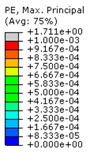
The dynamic response of the wall is presented in Figure 11, where a maximum relative displacement of 10.153 mm is observed, which corresponds to a drift of 0.338%. Table 3 presents the damages obtained and the corresponding principal strains. The contours of the maximum principal strain represent the accumulated damages caused by the seismic excitation. After the dynamic analysis, the damages were revealed to be concentrated at the first layers at the bottom (from two corners) and developed following inclined directions from the base to the top of the wall (Table 3).
In order to assess the seismic performance of the studied wall, the IDA (incremental dynamic analysis) method [33] was applied: the real signal was scaled at different amplitudes, respectively 70%, 50% and 30% amplitudes of the real signal, which corresponded to the maximum accelerations amax of 0.223g, 0.160g and 0.096g, respectively. The maximum drifts and the damage modes are illustrated in Figure 12 and Table 4.
4.4. Case of L-Form Cross-Section Wall
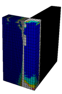
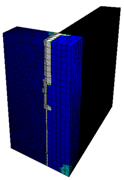
The wall was modeled by using eight-node volume elements (C3D8I). The mesh was discretized with a fine mesh measuring approximately 20 mm, which reached mesh convergence, except for the height direction of interlayers where a fine mesh of 5 mm was applied (Figure 13). In the out-of-plane direction of the transversal wall added (0.5-m-thickness, called “transversal flange”), the wall was meshed into five layers. The boundary conditions of the wall were the simple supports at the base. The origin of the system is at the point N1 (0,0,0). The coordinates of the center of mass and the rotation center at the point of connection with the supports are (1.81 m, 0.0625 m, 2.39 m) and (1.81 m, 0.0625 m, 0 m), respectively. The vertical loading applied on the top of a RE wall was of 0.1 MPa, similar to the previous case. The equivalent mass (15 tons) was also added at the top of the wall. The dynamic loading was introduced at the base of the wall. The natural frequencies obtained for four first vibrational mode from numerical simulation were 9.14Hz, 12.65Hz, 15.65Hz and 20.40Hz. The dynamic excitation was introduced to the model with rate of each 0.013 s (Δt). It is usually assumed that the rate is acceptable when Δt < T/8 where T is the period of the highest mode of interest, which is about 10–20 Hz for RE structures [16]. Three different signals were introduced which corresponded to 100%, 70% and 30% the amplitude of the real signal, which were equivalent to the maximum accelerations of 0.319 g, 0.223 g and 0.096 g, respectively.
The relative displacements and the drifts obtained are presented in Figure 14, Figure 15, Figure 16 and Figure 17. For all loading cases (amax = 0.319 g, 0.223 g and 0.096 g), the maximum drifts of the longitudinal flange were lower than that of the transversal flange (Figure 17). This result is comprehensible because the seismic signal was introduced in the direction parallel to the longitudinal flange, so this flange had an in-plane behavior, while the transversal flange had an out-of-plane response.
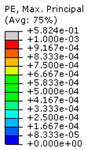
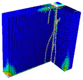
The failure patterns obtained are presented in Table 5. The important vertical cracks appeared in the connection between two flanges due to the out-of-plane movement of the lateral wall. For the case of 100% loading, the shear cracks also developed in the in-plane longitudinal flange. For the case of 30% loading, the damages considerably decreased in both flanges.
5. Discussions
Figure 18 and Figure 19 illustrate the variation of the relative displacements in function of time, obtained for the in-plane longitudinal wall in two cases: walls having rectangular and L-form cross-sections. It is observed that the L-form cross section wall had lower relative displacements when compared to the rectangular cross-section wall. This remark suggests that the presence of the transversal flange decreased contributed positively to the seismic performance of RE wall by decreasing its relative displacements under dynamic loadings. This result may come from the non-neglected thickness of RE wall being investigated (50-cm).
From Figure 17, if the drift limit of 0.3% is applied for RE buildings as the case of masonry [32], the L-form cross-section of a one-story RE building could have satisfying earthquake behavior for the ground motions with maximum accelerations until 0.223 g (both for the longitudinal flange with drift of 0.157% and the transversal flange with drift of 0.281%). The out-of-plane displacements of the transversal flange in this case are equivalent to the in-plane displacements of the rectangular cross-section wall. However, in the case of a whole building, the walls are linked between them by structural elements such as the beams on the top of the wall [32,34], so the out-of-plane displacement is expected to be reduced.
6. Conclusions and Prospects
In this study, a numerical approach using FEM and the time history analysis was used to study the seismic performance of the RE walls. The model was first validated by comparing the numerical results with that obtained from an experimental study. The results confirmed the importance to take into account the interlayers in the numerical model for RE walls under horizontal loadings.
The model was then applied to simulate a full-scale rectangular RE wall under in-plane seismic excitations with different amplitudes. The numerical outputs enabled us to calculate the relative displacements of RE walls and the corresponding drifts. The numerical damages obtained were also analyzed. Next, another wall with an L-form cross-section was modeled where a transversal flange was added to the rectangular wall studied before. The results showed that with the presence of the transversal flange, the damage mechanisms changed where the cracks concentrated essentially at the connection between two flanges; the relative displacements of the longitudinal flange decreased also significantly. Therefore, the study confirms that although the out-of-plane resistance of the walls are usually neglected in seismic design, this resistance in the case of RE walls—thanks to a high thickness level—can significantly contribute to the in-plane seismic resistance of the walls in the perpendicular directions.
The results also showed that the L-form cross-section of a one-story RE building could have satisfying earthquake behavior for the ground motions, with maximum accelerations until 0.223g (maximum drift of the longitudinal flange of 0.157% < 0.3% and maximum drift of the transversal flange of 0.281% < 0.3%). In practice, the drifts due to the out-of-plane displacements of the transversal flange are lower due to the presence of other structural elements, especially the beam on the top of the wall which links different walls. Further studies will be useful to assess these phenomena. Influences of the torsional effects will also important to investigate.
Author Contributions
Q.-B.B. proposed the first ideas; M.-P.T. performed one part of the numerical simulations under the supervision of Q.-B.B. and T.-T.B.; T.-L.B. and H.-A.L. worked on the parametric study in CDP model. The paper was written by Q.-B.B. and T.-T.B.
Funding
This research is funded by the Vietnam National Foundation for Science and Technology Development (NAFOSTED) under grant number 107.01-2017.22.
Conflicts of Interest
The authors declare no conflict of interest.
References
- Bui, Q.B.; Morel, J.C.; Reddy, B.V.V.; Ghayad, W. Durability of rammed earth walls exposed for 20 years to natural weathering. Build. Environ. 2009, 44, 912–919. [Google Scholar] [CrossRef]
- Bui, Q.B.; Morel, J.C.; Hans, S.; Walker, P. Effect of moisture content on the mechanical characteristics of rammed earth. Constr. Build. Mater. 2014, 54, 163–169. [Google Scholar] [CrossRef] [Green Version]
- Reddy, B.V.V.; Kumar, P.P. Embodied energy in cement stabilized rammed earth walls. Energy Build. 2010, 42, 380–385. [Google Scholar] [CrossRef]
- Walker, P.; Keable, R.; Martin, J.; Maniatidis, V. Rammed earth–design and construction guidelines. In BRE Bookshop; IHS BRE Press: Berkshire, UK, 2005. [Google Scholar]
- Morel, J.C.; Mesbah, A.; Oggero, M.; Walker, P. Building houses with local materials: Means to drastically reduce the environmental impact of construction. Build. Environ. 2001, 36, 1119–1126. [Google Scholar] [CrossRef]
- Soudani, L.; Fabbri, A.; Morel, J.C. Assessment of the validity of some common assumptions in hygrothermal modelling of earth based materials. Energy Build. 2016, 116, 498–511. [Google Scholar] [CrossRef]
- Allinson, D.; Hall, M. Hygrothermal analysis of a stabilized rammed earth test building in the UK. Energy Build. 2010, 42, 845–852. [Google Scholar] [CrossRef]
- Bui, T.T.; Bui, Q.B.; Limam, A.; Maximilien, S. Failure of rammed earth walls: From observations to quantifications. Constr. Build. Mater. 2014, 51, 295–302. [Google Scholar] [CrossRef] [Green Version]
- Bui, T.T.; Bui, Q.B.; Limam, A.; Morel, J.C. Modeling rammed earth wall using discrete element method. Contin. Mech. 2015, 28, 523–538. [Google Scholar] [CrossRef] [Green Version]
- Bui, Q.B. Assessing the rebound hammer test for rammed earth material. Sustainability 2017, 9. [Google Scholar] [CrossRef]
- Cheah, J.S.J.; Walker, P.; Heath, A.; Morgan, T.K.K.B. Evaluating shear test methods for stabilized rammed earth. Constr. Mater. 2012, 165, 325–334. [Google Scholar] [CrossRef]
- Ciancio, D.; Augarde, C. Capacity of unreinforced rammed earth walls subject to lateral wind force: Elastic analysis versus ultimate strength analysis. Mater. Struct. 2013, 46, 1569–1585. [Google Scholar] [CrossRef]
- Miccoli, L.; Oliveira, D.V.; Silva, R.A.; Muller, U.; Schueremans, L. Static behavior of rammed earth: Experimental testing and finite element modeling. Mater. Struct. 2014, 48, 3443–3456. [Google Scholar] [CrossRef]
- Silva, R.A.; Oliveira, D.V.; Miranda, T.; Cristelo, N.; Escobar, M.C.; Soares, E. Rammed earth construction with granitic residual soils: The case study of northern Portugal. Constr. Build. Mater. 2013, 47, 181–191. [Google Scholar] [CrossRef] [Green Version]
- Miccoli, L.; Drougkas, A.; Müller, U. In-plane behavior of rammed earth under cyclic loading: Experimental testing and finite element modelling. Eng. Struct. 2016, 125, 144–152. [Google Scholar] [CrossRef]
- Bui, Q.B.; Hans, S.; Morel, J.C.; Do, A.P. First exploratory study on dynamic characteristics of rammed earth buildings. Eng. Struct. 2011, 33, 3690–3695. [Google Scholar] [CrossRef]
- Gomes, M.I.; Lopes, M.; Brito, J. Seismic resistance of earth construction in Portugal. Eng. Struct. 2011, 33, 932–941. [Google Scholar] [CrossRef] [Green Version]
- El-Nabouch, R.; Bui, Q.B.; Plé, O.; Perrotin, P. Assessing the in-plane seismic performance of rammed earth walls by using horizontal loading tests. Eng. Struct. 2017, 145, 153–161. [Google Scholar] [CrossRef]
- Bui, Q.B.; Bui, T.T.; Limam, A. Assessing the seismic performance of rammed earth walls by using discrete elements. Cogent Eng. 2016, 3, 1200835. [Google Scholar] [CrossRef]
- ABAQUS Version 6.12 Documentation. ABAQUS Analysis User’s Manual 6.12-EF; Dassault Systems Simulia Corp.: Providence, RI, USA, 2013. [Google Scholar]
- El-Nabouch, R.; Bui, Q.B.; Perrotin, P.; Plé, O. Shear parameters of rammed earth material: Results from different approaches. Adv. Mater. Sci. Eng. 2018. [Google Scholar] [CrossRef]
- Foti, D.; Ivorra, S.; Vacca, V. In plane behavior of a masonry stone wall with hexagonal blocks. In Proceedings of the 16th International Brick and Block Masonry Conference (IBMAC 2016), Padova, Italy, 26–30 June 2016; pp. 1587–1591. [Google Scholar]
- Bui, Q.B.; Limam, A.; Bui, T.T. Dynamic discrete element modelling for seismic assessment of rammed earth walls. Eng. Struct. 2018, 175, 690–699. [Google Scholar] [CrossRef]
- Nasiri, E.; Liu, Y. Development of a detailed 3D FE model for analysis of the in-plane behavior of masonry infilled concrete frames. Eng. Struct. 2017, 143, 603–616. [Google Scholar] [CrossRef]
- Lubliner, J.; Oliver, J.; Oller, S.; Oñate, E. A plastic-damage model for concrete. Int. J. Solids Struct. 1989, 25, 299–326. [Google Scholar] [CrossRef]
- Lee, J.; Fenves, G. Plastic-Damage Model for Cyclic Loading of Concrete Structures. J. Eng. Mech. 1998, 124, 892–900. [Google Scholar] [CrossRef]
- Genikomsou, A.S.; Polak, M.A. Finite element analysis of punching shear of concrete slabs using damaged plasticity model in ABAQUS. Eng. Struct. 2015, 98, 38–48. [Google Scholar] [CrossRef]
- Cornelissen, H.A.W.; Hordijk, D.A.; Reinhardt, H.W. Experimental Determination of Crack Softening Characteristics of Normalweight and Lightweight Concrete; HERON; Delft University of Technology: Delft, The Netherlands, 1986; Volume 31. [Google Scholar]
- FIB. FIB Model Code for Concrete Structures; Wiley-VCH Verlag GmbH & Co. KGaA: Weinheim, Germany, 1990. [Google Scholar]
- Feenstra, P.H.; Borst, R. Computational Aspects of Biaxial Stress in Plain and Reinforced Concrete; Delft University Press: Delft, The Netherlands, 1993. [Google Scholar]
- El-Nabouch, R.; Bui, Q.B.; Plé, O.; Perrotin, P. Characterizing the shear parameters of rammed earth material by using a full-scale direct shear box. Constr. Build. Mater. 2018, 171, 414–420. [Google Scholar] [CrossRef]
- Calvi, G.M. A displacement-based approach for vulnerability evaluation of classes of buildings. J. Earthq. Eng. 1999, 3, 411–438. [Google Scholar] [CrossRef]
- Vamvatsikos, D.; Cornell, C.A. Incremental dynamic analysis. Earthq. Engng Struct. Dyn. 2002, 31, 491–514. [Google Scholar] [CrossRef]
- Walker, P.; Dobson, S. Pullout Tests on Deformed and Plain Rebars in Cement-Stabilized Rammed Earth. J. Mater. Civ. Eng. 2001, 13, 291–297. [Google Scholar] [CrossRef]
Figure 1.
Typical behavior of earthen (intralayers) in the CDP model for: (a) axial compressive strength; (b) tension strength; (c) typical surface of stress conditions.
Figure 1.
Typical behavior of earthen (intralayers) in the CDP model for: (a) axial compressive strength; (b) tension strength; (c) typical surface of stress conditions.

Figure 2.
Compression and softening model [30].
Figure 2.
Compression and softening model [30].

Figure 3.
Failure criterion of Mohr-Coulomb.
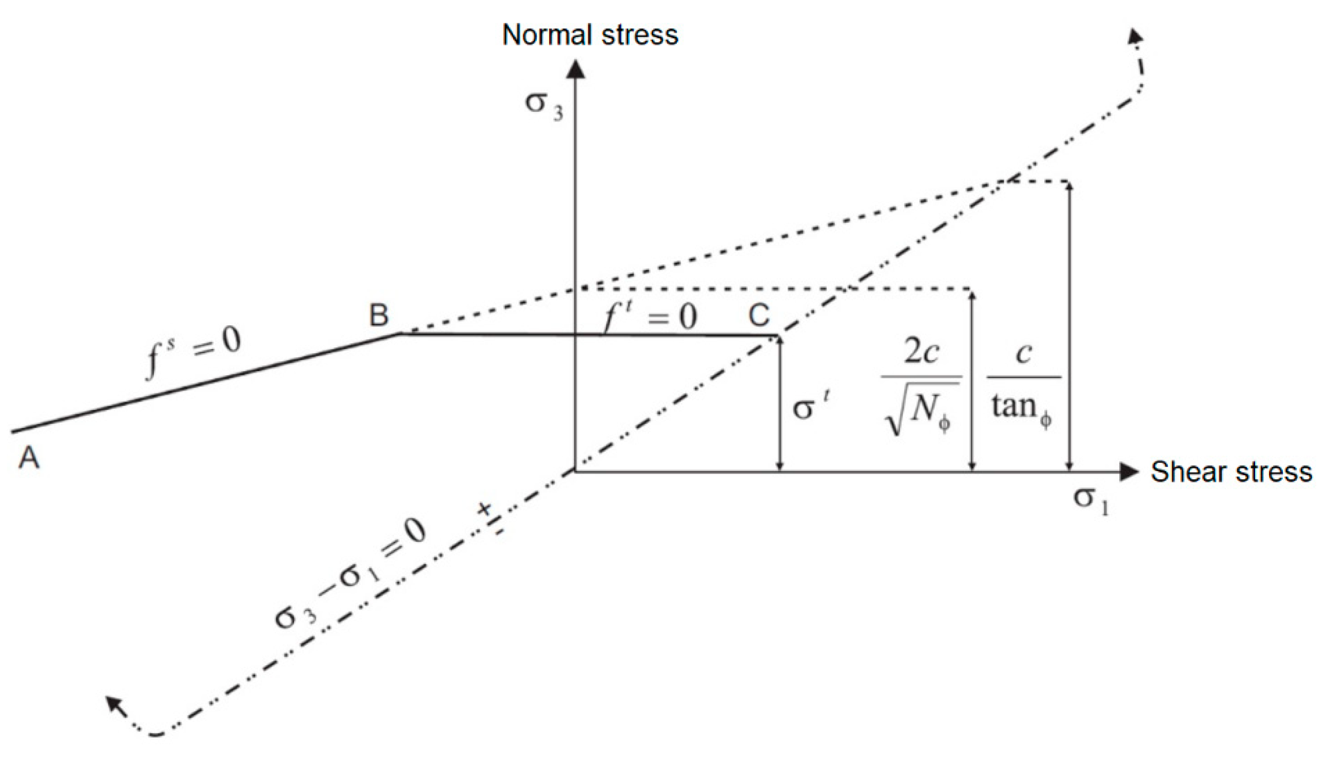
Figure 4.
Mesh of the wall, in the case without (a) and with (b) interlayers.
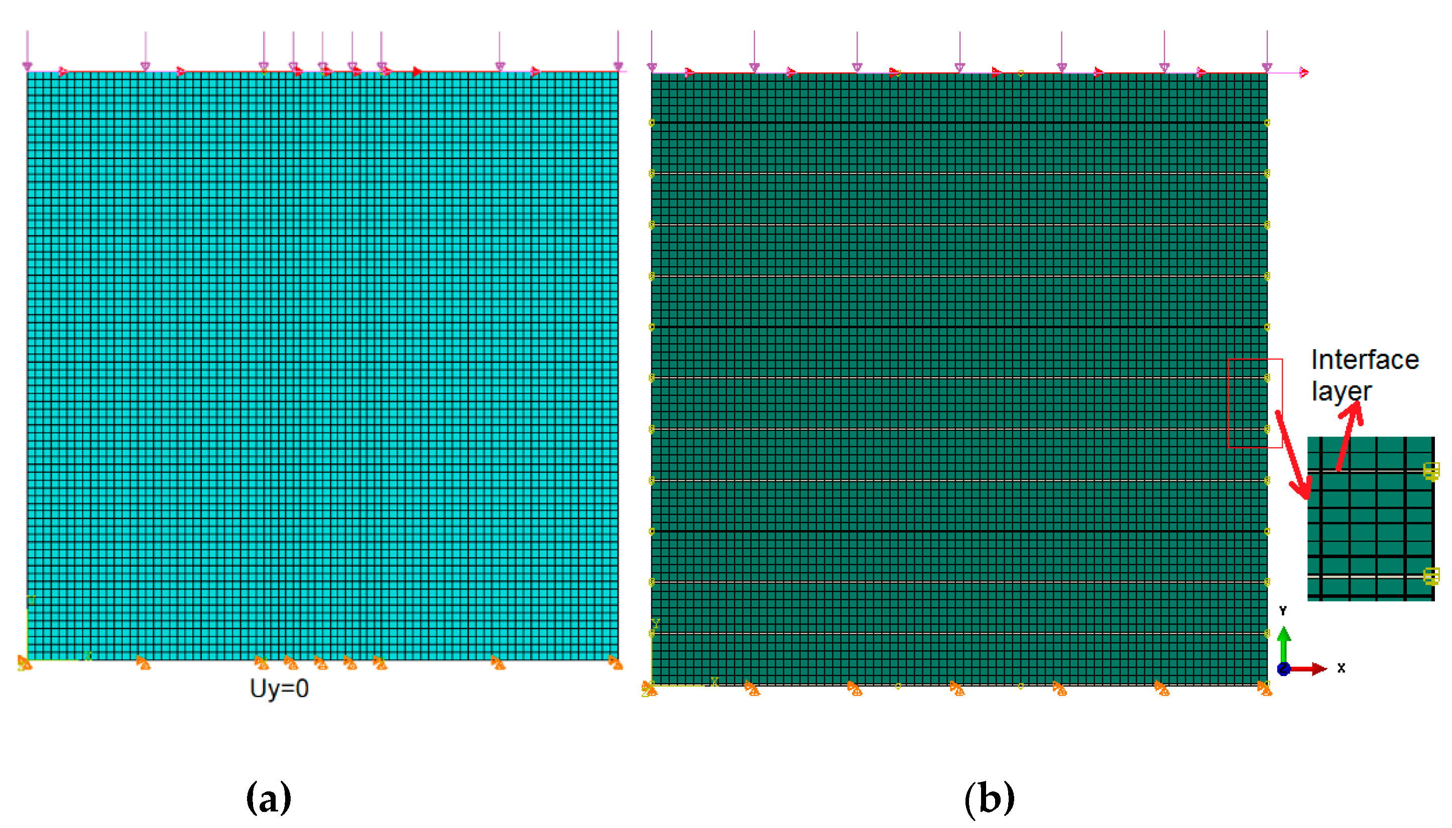
Figure 5.
Influence of the dilation angle on the numerical result.

Figure 6.
Numerical and experimental horizontal load/displacement curves.
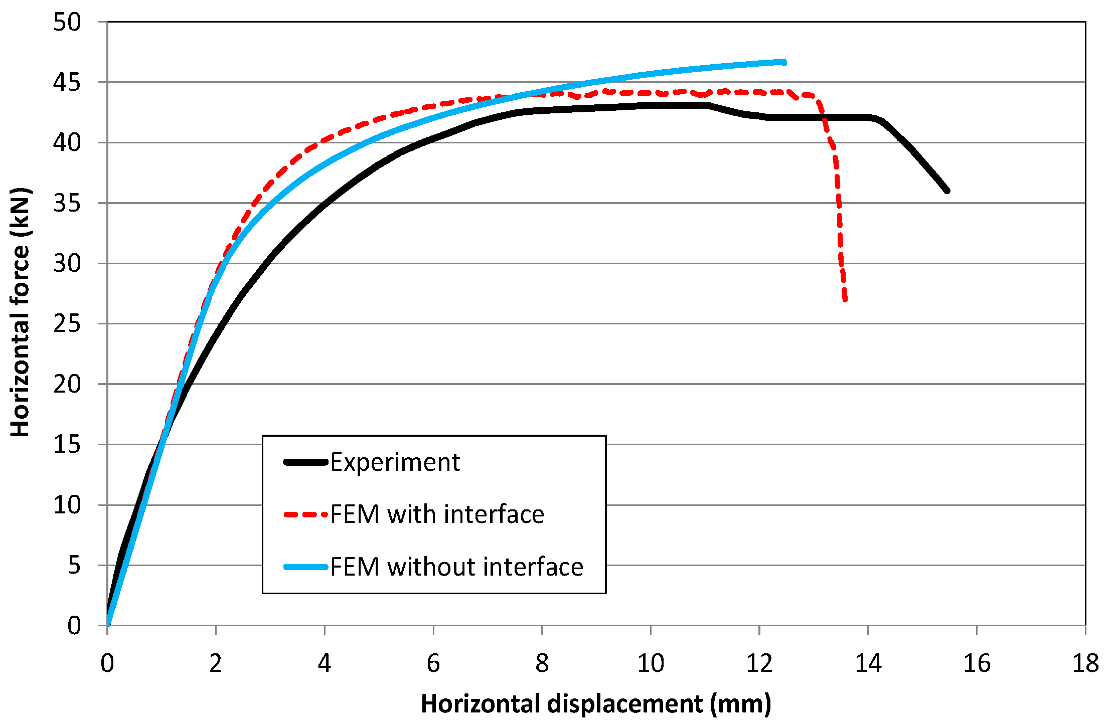
Figure 7.
Failure modes obtained by: experiment (a); model without interlayers (b) and with interlayers (c).
Figure 7.
Failure modes obtained by: experiment (a); model without interlayers (b) and with interlayers (c).
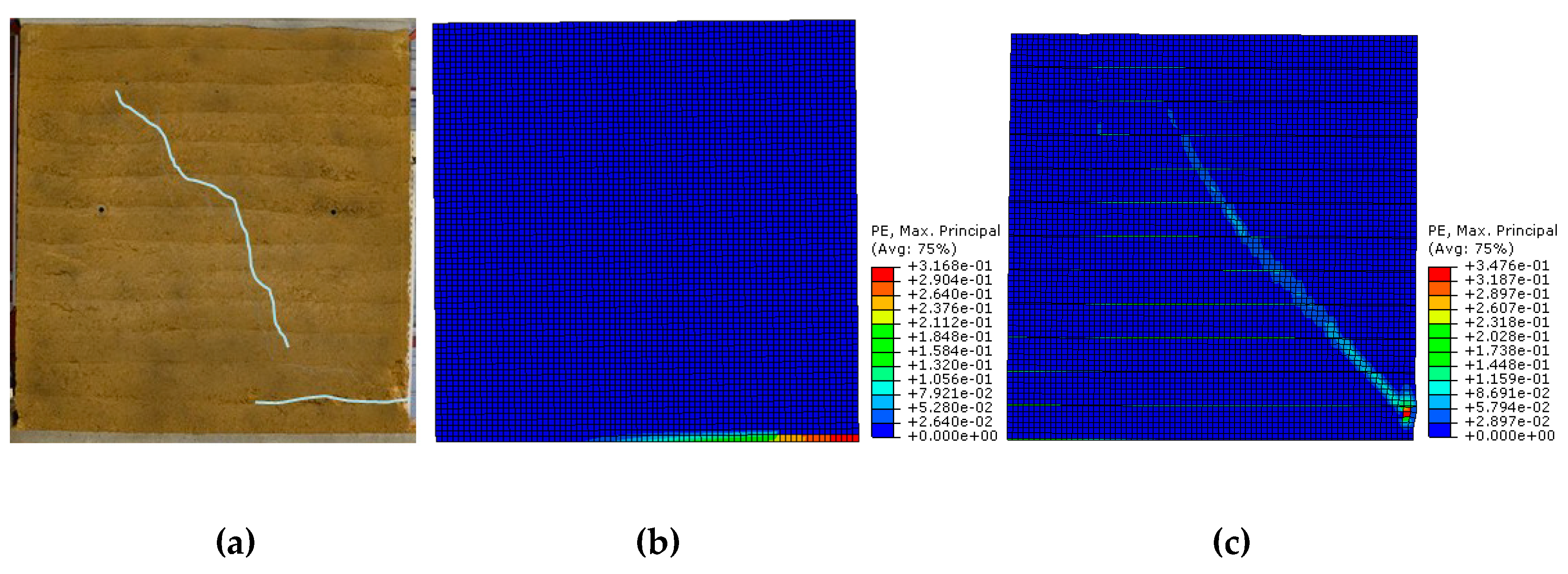
Figure 8.
Models of two RE walls: (a) without and (b) with lateral wall. Dimensions in mm.
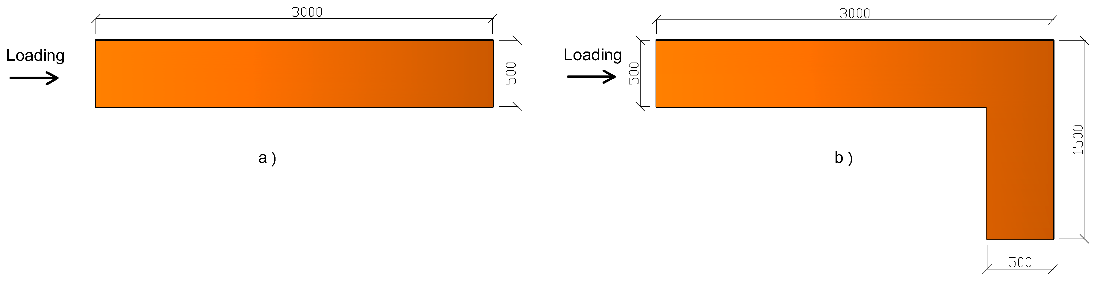
Figure 9.
NS component of El Centro earthquake 1940.
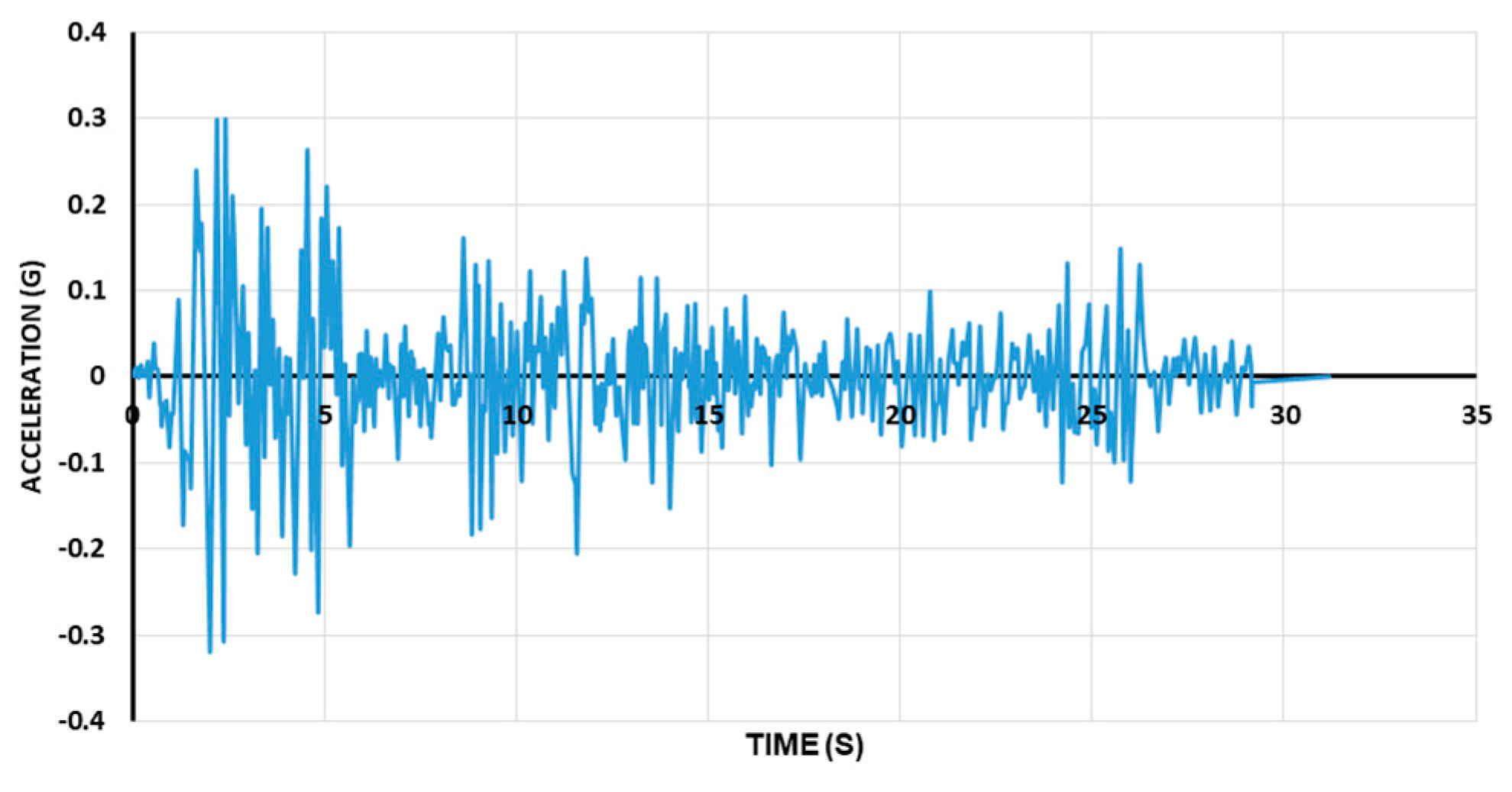
Figure 10.
Mesh and boundary conditions of a rectangular cross-section RE wall.

Figure 11.
Relative displacements obtained in function of time, for the case of 100% excitation.

Figure 12.
Drift vs acceleration: one-story-building.
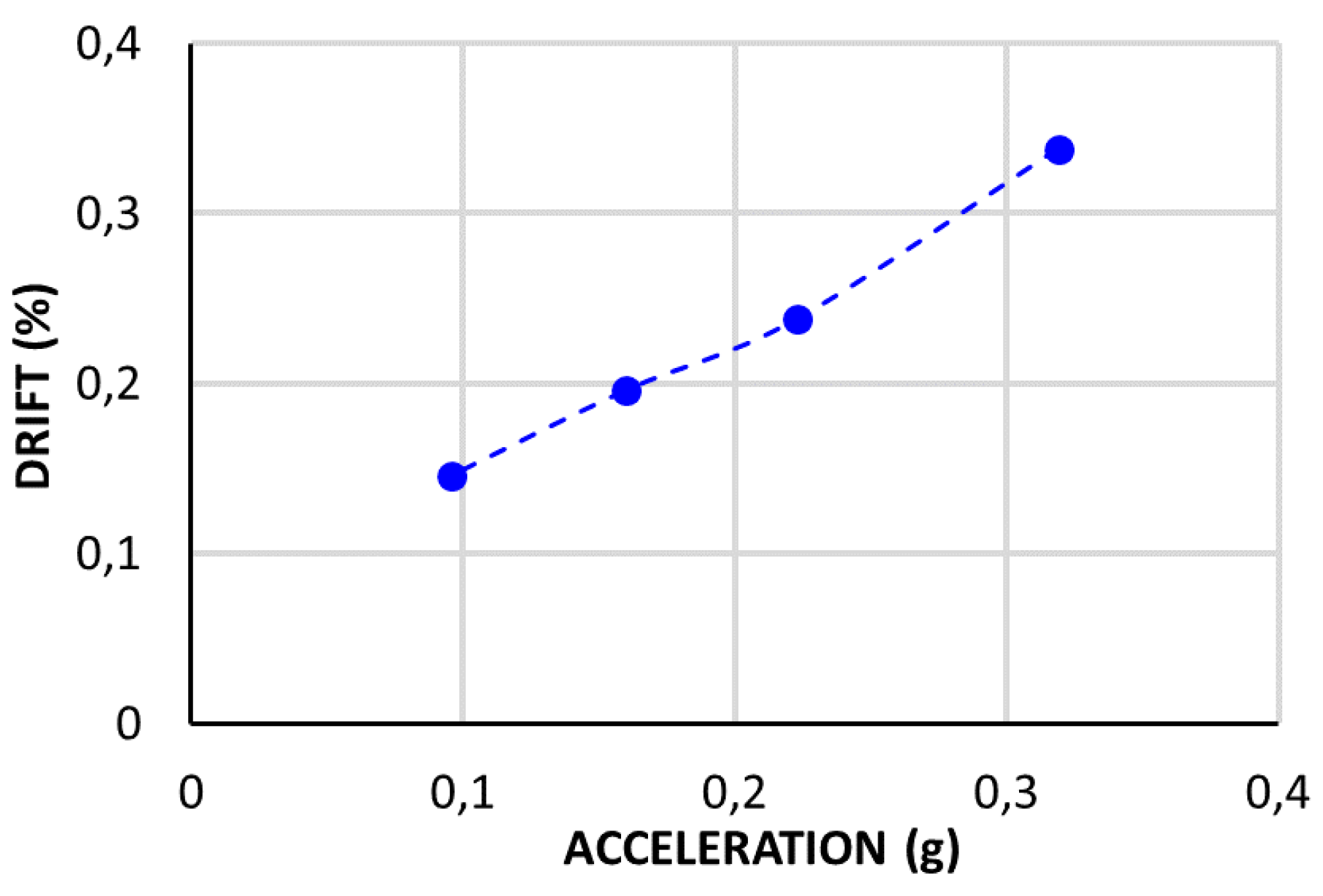
Figure 13.
L-form RE wall having a longitudinal flange and a transversal flange.
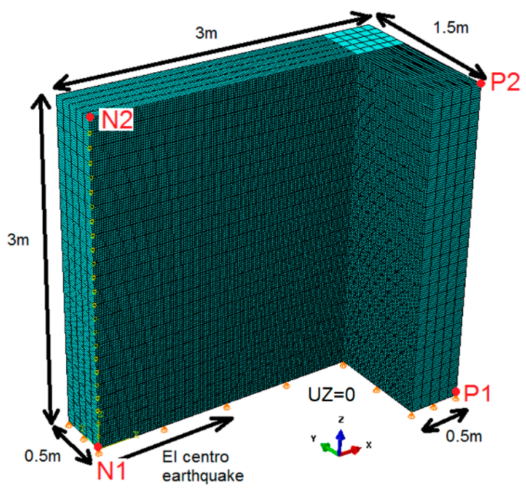
Figure 14.
Variation of the relative displacements in function of time, for the case of 100% real excitation: (a) points N: in-plane of the longitudinal wall; (b) points P: out-of-plane of the transversal wall.
Figure 14.
Variation of the relative displacements in function of time, for the case of 100% real excitation: (a) points N: in-plane of the longitudinal wall; (b) points P: out-of-plane of the transversal wall.
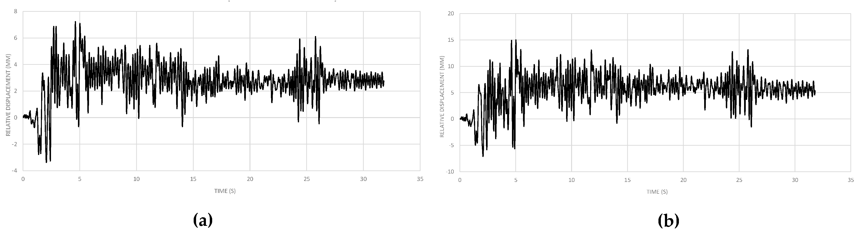
Figure 15.
Variation of the relative displacements in function of time, for the case of 70% real excitation: (a) points N: in-plane of the longitudinal wall; (b) points P: out-of-plane of the transversal wall.
Figure 15.
Variation of the relative displacements in function of time, for the case of 70% real excitation: (a) points N: in-plane of the longitudinal wall; (b) points P: out-of-plane of the transversal wall.
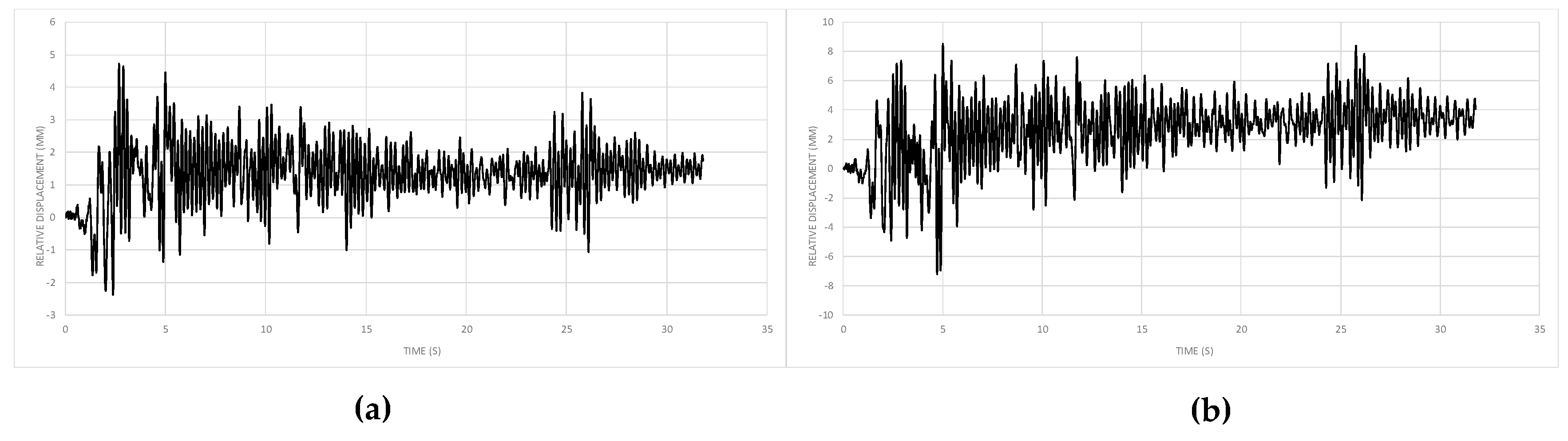
Figure 16.
Variation of the relative displacements in function of time, for the case of 30% real excitation: (a) points N: in-plane of the longitudinal wall; (b) points P: out-of-plane of the transversal wall.
Figure 16.
Variation of the relative displacements in function of time, for the case of 30% real excitation: (a) points N: in-plane of the longitudinal wall; (b) points P: out-of-plane of the transversal wall.

Figure 17.
Evolution of the drift in function of acceleration.

Figure 18.
Case of 100% excitation, for rectangular and L-form cross-sections.

Figure 19.
Case of 30% excitation, for rectangular and L-form cross-sections.


Table 1.
Gf0 depending on dmax.
| dmax (mm) | Gf0 (Nmm/mm2) |
|---|---|
| 8 | 0.025 |
| 16 | 0.030 |
| 32 | 0.058 |
Table 2.
Concrete damaged plasticity parameters.
| Parameter | Description | Default Value |
|---|---|---|
| Ψ | Dilation angle | User-defined |
| ∈ | Flow potential eccentricity | 0.1 |
| Ratio of initial equibiaxial compressive yield stress to initial uniaxial compressive yield stress | 1.16 | |
| Kc | Ratio of the second stress invariant on the tensile meridian | 0.6667 |
Table 3.
Results obtained for the cases of 100% excitation.
| Max. Relative Displacement | Max. Drift | Max. Principal Strain | |
|---|---|---|---|
| 10.153 mm | 0.338% |  |  |
Table 4.
Damages after different amplitudes of excitation.
| amax | Max Principal Strain | |
|---|---|---|
| 0.096 g (30% loading) |  | 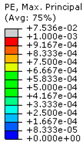 |
| 0.160 g (50% loading) |  |  |
| 0.223 g (70% loading) | 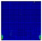 |  |
| 0.319 g (100% loading) | 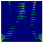 |  |
Table 5.
Evolution of damage for the cases of 100%, 70% and 30% of the real excitation.
| 100% Loading (amax = 0.319 g) | 70% Loading (amax = 0.223 g) | 30% Loading (amax = 0.096 g) |
|---|---|---|
 |  |  |
 |  |  |
 |  |  |
© 2019 by the authors. Licensee MDPI, Basel, Switzerland. This article is an open access article distributed under the terms and conditions of the Creative Commons Attribution (CC BY) license (http://creativecommons.org/licenses/by/4.0/).
Share and Cite
MDPI and ACS Style
Bui, Q.-B.; Bui, T.-T.; Tran, M.-P.; Bui, T.-L.; Le, H.-A. Assessing the Seismic Behavior of Rammed Earth Walls with an L-Form Cross-Section. Sustainability 2019, 11, 1296. https://doi.org/10.3390/su11051296
AMA Style
Bui Q-B, Bui T-T, Tran M-P, Bui T-L, Le H-A. Assessing the Seismic Behavior of Rammed Earth Walls with an L-Form Cross-Section. Sustainability. 2019; 11(5):1296. https://doi.org/10.3390/su11051296
Chicago/Turabian StyleBui, Quoc-Bao, Tan-Trung Bui, Mai-Phuong Tran, Thi-Loan Bui, and Hoang-An Le. 2019. "Assessing the Seismic Behavior of Rammed Earth Walls with an L-Form Cross-Section" Sustainability 11, no. 5: 1296. https://doi.org/10.3390/su11051296
Note that from the first issue of 2016, this journal uses article numbers instead of page numbers. See further details here.