Optimum Turf Grass Irrigation Requirements and Corresponding Water- Energy-CO2 Nexus across Harris County, Texas


1
College of Agriculture and Human Sciences, Cooperative Agricultural Research Center, Prairie View A&M University, Prairie View, TX 77446, USA
2
Office of Research, Innovation and Sponsored Programs, Prairie View A&M University, Prairie View, TX 77446, USA
*
Author to whom correspondence should be addressed.
Sustainability 2019, 11(5), 1440; https://doi.org/10.3390/su11051440
Submission received: 24 December 2018
/
Revised: 28 February 2019
/
Accepted: 5 March 2019
/
Published: 8 March 2019
(This article belongs to the Special Issue Water-Energy Sustainable Urban Development)
Abstract
:Harris County is one of the most populated counties in the United States. About 30% of domestic water use in the U.S. is for outdoor activities, especially landscape irrigation and gardening. Optimum landscape and garden irrigation contributes to substantial water and energy savings and a substantial reduction of CO2 emissions into the atmosphere. Thus, the objectives of this work are to (i) calculate site-specific turf grass irrigation water requirements across Harris County and (ii) calculate CO2 emission reductions and water and energy savings across the county if optimum turf grass irrigation is adopted. The Irrigation Management System was used with site-specific soil hydrological data, turf crop water uptake parameters (root distribution and crop coefficient), and long-term daily rainfall and reference evapotranspiration to calculate irrigation water demand across Harris County. The Irrigation Management System outputs include irrigation requirements, runoff, and drainage below the root system. Savings in turf irrigation requirements and energy and their corresponding reduction in CO2 emission were calculated. Irrigation water requirements decreased moving across the county from its north-west to its south-east corners. However, the opposite happened for the runoff and excess drainage below the rootzone. The main reason for this variability is the combined effect of rainfall, reference evapotranspiration, and soil types. Based on the result, if the average annual irrigation water use across the county is 25 mm higher than the optimum level, this will result in 10.45 million m3 of water losses (equivalent water use for 30,561 single families), 4413 MWh excess energy use, and the emission of 2599 metric tons of CO2.
1. Introduction
Texas is the second most populated state and has the second largest economy in the United States. Texas experienced the largest population increase, 399,734 residents, in the country between July 2016 and July 2017, according to U.S. Census Bureau estimates. The Texas population is also predicted to double by 2070 compared to its level at 2010, with the Dallas–Fort Worth metropolitan area (Tarrant County) and Houston metropolitan area (Harris County) accounting for more than half of the state’s total projected population growth [1]. Currently, 85 percent of Texans live in urban areas, and Texas is expected to have more than 90 percent of its 2010–2050 total population growth live in urban areas [2]. Population and steady economic growth have led to increasing water and energy demand in Texas. According to the Texas Water Development Board (TWDB), the annual water demand in Texas is expected to increase by 17 percent, from about 22.7 billion m3 per year in 2020 to about 26.64 billion m3 in 2070, while the existing water supplies (surface water, groundwater, and reused water) are projected to decrease by about 11 percent, from 18.75 billion m3 per year in 2020 to about 16.78 billion m3 in 2070 [1]. The water demand in Harris County is projected to increase by 37 percent between 2020 and 2070 [1].
Water is a key component for energy (e.g., nuclear, biofuels, and fossil) resource extraction, energy conversion, refining, electricity generation (hydropower, thermoelectric, and renewable technologies), and transportation. The availability and locations of water resources determine the technology, sites, and types of energy facilities. On the other hand, energy is used to withdraw, supply, treat, and use freshwater resources for different sectors, e.g., domestic, agriculture, and industries. Energy is also needed to convey, treat, and distribute wastewater. In the United States, 13% of energy consumption is used to supply, treat, and use water, meaning that water resource management and practices can significantly affect water and energy use and greenhouse gas emissions [3,4]. Therefore, water, energy, and carbon dioxide are inter-connected and form a nexus. Multiple studies have reported the statistically significant positive association between energy consumption and greenhouse gases emissions. Saidi and Hammami [5] investigated the impact of economic growth and CO2 emissions on energy consumption for 58 countries over the 1990–2012 period; their results showed that economic growth has a positive impact on energy consumption. Menyah and Rufael [6] found a positive effect of CO2 emissions on energy consumption in South Africa. Similarly, Niu et al. [7] showed a positive relationship between energy consumption and CO2 emissions in eight Asian–Pacific countries. Results from Arouri et al. [8] showed the positive and significant impact of energy consumption on CO2 emissions in 12 Middle East and North African Countries (MENA) over the 1981–2005 period. Water and energy uses and CO2 emissions are closely linked; as a consequence, water conservation strategies can reduce potential energy consumption and ultimately decrease carbon dioxide emissions.
In order to meet the future water demand in Texas and prevent serious economic losses resulting from water shortages, TWDB planning groups recommend water management strategies and associated projects, such as adopting conservation measures; drilling new groundwater wells; increasing wastewater reuse, desalination of seawater, and brackish groundwater; and/or building new surface water reservoirs. Optimum irrigation water management practices play a crucial role in water conservation. Following such practices, irrigation water is applied at the appropriate amount that meets the need of the growing plants without excess losses below the root zone or as surface runoff. Consequently, water conservation saves energy and reduces carbon dioxide emissions.
Currently, municipal/urban areas use 27% of Texas freshwater resources are the second largest category of water users after irrigated agriculture, which uses 51% of Texas freshwater resources. Urban/municipal water use is expected to increase to 39% in the next five decades as a result of expected population growth [1]. In 2020, Harris County will have the highest annual municipal water needs (1011 million m3) across the state, and in 2070, the municipal water demands will reach more than 1295 million m3 [1]. Within this use category (municipal/urban), lawn and landscape water uses are significant but largely unmeasured. Landscape plants (e.g., grass, plants, and trees) are vital elements of urban environments and provide an array of economic, environmental, human health, and social benefits [9]. A recent study across selected Texas cities has shown that about 31% of single-family residential annual water consumption was dedicated to outdoor purposes, mostly landscape irrigation, during the 2004–2011 period [10]. Based on information from some of the largest cities and municipal water suppliers, the average annual irrigation in Texas is 762 mm which matches with the average difference between historical annual precipitation and reference evapotranspiration (ETo) across the state [11]. Although landscape planting uses significant amounts of fresh municipal/urban water, there have been very few studies directed to investigate optimum urban water management and its impact on energy conservation and CO2 emission reduction.
Therefore, the objectives of this work are (i) to calculate site-specific optimum irrigation water requirements for turf grass across Harris County and (ii) to estimate water and energy savings and reductions in CO2 emissions if optimum turf grass irrigation is adopted. The significant contribution of this work is to calculate the irrigation water needs for urban landscapes in Harris County and offer strategies and management practices that can significantly increase water use efficiency, reduce excessive water losses, and corresponding CO2 emission reduction.
2. Materials and Methods
2.1. Study Area and Data Used
The study area is Harris County in Texas which is located in the southeastern part of the state, near Galveston Bay (see Figure 1). According to Census (2010), Harris County, with a population of over 4.1 million, is the most populous county in Texas and the third most populous county in the United States. Houston, the largest city in Texas and the fourth most populous city in the U.S., is Harris County’s seat and has a total area of 4600 km2, of which 96% is land and 4% is water. The major land covers are urban and built-up areas, cropland/natural vegetation mosaics, woody savannas, croplands, grasslands, mixed forests, sea, and land water bodies [12]. Two nearby large water bodies in Harris County are Galveston Bay to the east and the Gulf of Mexico, which is approximately 80 km, to the south-east [13]. Although it is a highly urbanized county, Harris County’s urban areas’ demand for freshwater resources continues to increase at a high rate, especially in its north-west areas. The county’s climate is humid and subtropical which makes summers hot and humid and winters mild to cool. The annual average precipitation is 1200 mm.
Daily precipitation, minimum temperature (Tmin), maximum temperature (Tmax), wind speed, relative humidity, and solar radiation were obtained from the National Centers for Environmental Prediction Climate Forecast System Reanalysis (NCEP–CFSR) global weather data [14] for the period of 1978 to 2013. The CFSR was designed and executed as a global, high-resolution, coupled atmosphere–ocean–land surface–sea ice system to provide the best estimate of the state of these coupled domains over the 36-year period; the daily NCEP-CFSR data are available online and have been widely used in many studies [15,16,17].
Daily reference evapotranspiration (ETo) data were calculated using the modified Food and Agriculture Organization’s Penman–Monteith equation (FAO-ETo) [18]:
where ETo is the reference evapotranspiration (mm day−1), Rn is the net radiation at the crop surface (MJ m−2 day−1), G is the soil heat flux density (MJ m−2 day−1), T is the air temperature at 2 m height (°C), es is the saturation vapor pressure (kPa), ea is the actual vapor pressure (kPa), es − ea is the saturation vapor pressure deficit (kPa), ∆ is the slope vapor pressure curve (kPa °C−1), γ is the psychrometric constant (kPa °C−1), and u2 is the wind speed at height 2 m (m s−1).
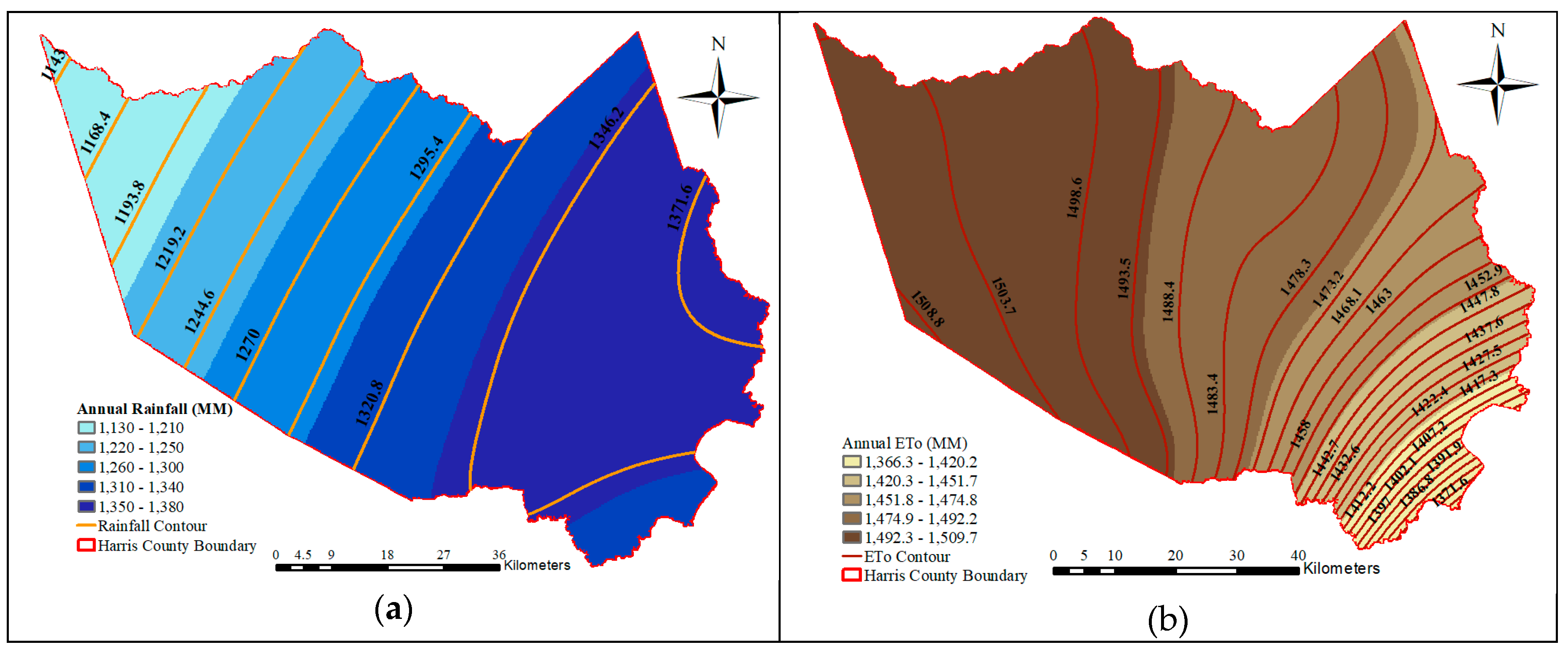
The annual spatial distributions of precipitation and reference evapotranspiration (Figure 2a,b) were computed using the long-term daily data (1978 to 2013). The average annual rainfall across the county decreases from 1366 mm in its south-east part to 1139 mm in the north-west part (Figure 2a). The reference evapotranspiration demand across the county varies in the opposite direction of rainfall from 1366 mm in the south-east to 1500 mm in the north-west part of the county (see Figure 2b).
The soil and land cover data used were obtained from the Soil Survey Geographic (SSURGO) database [19] and the National Land Cover Database (NLCD), respectively. Based on the land cover map (Figure 3a), Harris County is highly urbanized with 21% of its area classified as developed open space (Figure 3b), 27% as developed low intensity (Figure 3c), 36% as developed medium intensity (Figure 3d), and 17% as developed high intensity (Figure 3e). Using the land cover data, we estimated that 10%, 30%, 10%, and 5% of the open space, low-intensity, medium-intensity, and high-intensity areas of the land cover are irrigated, respectively.
2.2. Optimum Irrigation Water Requirement for Turf Grass
Although there is no detailed information on Irrigation Water Requirement (IWR) for turf grass in Harris County, it can be calculated based on the site-specific historical daily weather data (e.g., rainfall and evapotranspiration), soil hydrologic properties (mainly water holding capacity and Soil Conservation Service (SCS) curve number), and plant water uptake data using IManSys databases [20].
IManSys has been used in several studies to calculate current IWRs for turf grass in Hawaii, Arizona, and Florida [21] and future IWRs for seed corn and coffee [22] and for citrus across the major global citrus production areas [23]. Also, an advanced version of IManSys, IWREDSS, has been used by Hawaii’s Commission on Water Resource Management to calculate crop water allocation across the state; a detailed description of the model was presented by Fares [24].
IManSys is a numerical simulation model that calculates IWR for any annual or perennial crop using the water balance approach [25] and based on site-specific crop and soil parameters and historical weather data. IManSys provides users with runoff, drainage, canopy interception, effective rainfall, and crop evapotranspiration based on plant growth parameters, soil properties, irrigation system, and long-term weather data (precipitation and ETo). If ETo data is unavailable, IManSys calculates evapotranspiration using limited weather data, e.g., a temperature-based model, or using complete weather data, e.g., the FAO Penman–Monteith method (Equation 1). The FAO Penman–Monteith equation implemented in the model accounts for climate change effects, so the user should specify the carbon dioxide concentration for which ETo will be calculated [22]; as such, IManSys accounts for climate change effects and water management practices on IWRs. However, we did not consider climate change effects in this study. IManSys was implemented in the JAVA object-oriented language. The model outputs include detailed net and gross IWRs and all water budget components at different time scales (daily, weekly, biweekly, monthly, and annually). IManSys uses calculated long-term daily IWRs to calculate statistical parameters and probabilities of occurrence of IWRs for various time periods based on non-exceedance drought probability, which is calculated from a conditional probability model that uses the type I extreme value distribution for positive non-zero irrigation values.
In IManSys, the simulated soil profile depth is assumed to be equal to the crop root zone depth. The simulated plant root zone is divided equally into two zones, an irrigated (upper 50%) and a non-irrigated (lower 50%) zone, based on the common practice of irrigating only the upper portions of the crop root zone where most of the roots are located [26]. It is assumed that 70% and 30% of crop ET are extracted from the irrigated and non-irrigated zones, respectively, when water is available for crops grown on non-restrictive soil profiles [26]. Multiple databases, e.g., soil, plant growth parameters, crop factors, irrigation system efficiencies, and canopy interception, are available in IManSys databases. Crop parameters including effective rooting depths, crop water use coefficients (Kc), duration of cropping season, and allowable water depletion for 29 major annual and 28 perennial crops are provided along with common irrigation systems and their corresponding irrigation efficiencies. The following data were used for turf grass in this study: total root zone depth of 60 cm, irrigated root zone depth of 30 cm, Kc value of 1 for each month of the year [26], and a multiple-sprinkler irrigation system with an irrigation efficiency of 0.75.
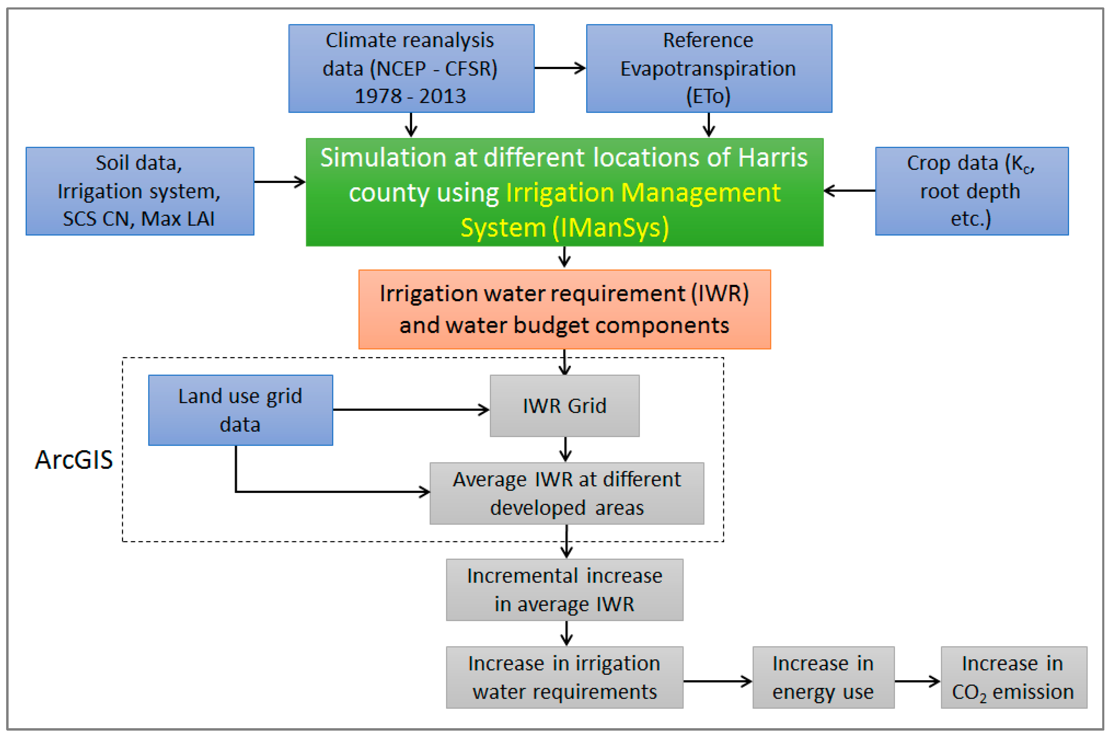
Soil properties, water features, and engineering properties of soils across Harris County including soil name, soil texture type, soil layer number, soil layer depth, hydrologic soil group, upper and lower bound of the water table, and maximum and minimum water holding capacity of each layer used in this study were extracted from the Soil Survey Geographic Database of the U.S. Department of Agriculture-Natural Resources and Conservation Service (USDA-NRCS) Web Soil Survey website. Figure 4 shows the flow chart that summarizes the overall analysis using the IManSys model and different input data.
2.3. Energy Requirement for Irrigation and Carbon Dioxide Emission
Energy and CO2 emission calculations were made based on the following information gathered from different sources. According to the Texas Water Development Board, drinking water in Harris County is a blend of 2/3 surface water and 1/3 groundwater. Groundwater and surface water have different energy footprints. An EPA report documented that energy use to supply domestic water from groundwater sources use is 476 kWh per thousand m3. However, domestic water generated from surface water sources requires 396 kWh per thousand m3 [27]. Texas energy is generated mainly from coal (36%), natural gas (41.1%), nuclear (11.6%), wind (10.6%), and other sources which account for about 0.8% based on a report from Electric Reliability Council of Texas, Inc. [28]. The carbon dioxide emitted per kWh energy produced in Texas is 984 g for coal, 549 g for natural gas, 68 g for nuclear, 9 g for wind, and 14 g for hydro and other sources [29,30]. In this study, the above values were used to determine the mass of CO2 per unit kWh energy used.
3. Results and Discussion
We selected 48 locations across Harris County to simulate turf grass IWRs (see Figure 5). These locations were chosen to cover all four major land covers, county major soil types, and spatial and temporal hydrological variabilities (temperature and rainfall) of the turf grass landscape.
Annual and monthly IWRs for turf grass were calculated for all the 48 locations, then the regularized spline method through ArcGIS 10 (ESRI, Redland, CA) was used to compute the spatial interpolation of the major water budget components, including irrigation requirement, runoff, rainfall, evapotranspiration, interception, and drainage. The detailed annual water budgets for four locations are plotted to illustrate the effect of spatial distribution (Figure 5) on turf grass irrigation water requirements and the main water budget components (Figure 6). The results show the strong impact of spatial variability on the water budget components. As we move from the north-west to the south-east of Harris County, crop evapotranspiration and irrigation water requirements decline by almost 90 and 215 mm, respectively. However, rainfall increases from 1130 mm to 1350 mm, and runoff also increases from 43 mm to 193 mm. The average canopy interception and drainage are 74 mm and 194 mm, respectively.
Figure 7 and Figure 8 represent the spatial interpolation of the annual irrigation water requirement and surface runoff across the county, respectively. The figures illustrate the strong spatial variability of the variables across Harris County. IWR decreases from its highest level in the north-west of the county to its lowest amount in the south-east corner of the county in response mainly to the combined effect of rainfall increase and reference evapotranspiration decrease. The estimated annual IWR varies from 686 to 940 mm with a county average of 790 mm, which is very close to the statewide landscape irrigation water requirements suggested by Cabrera [11]. The opposing spatial variability trends in evapotranspiration and rainfall divide the county into three hydrological areas. The north-west part of the county is characterized by relatively low rainfall and high ETo demands; however, the central part of the county is characterized by a relatively moderate rainfall and high ETo. Contrary to the other two regions, the east of the county has high rainfall and low ETo demands.
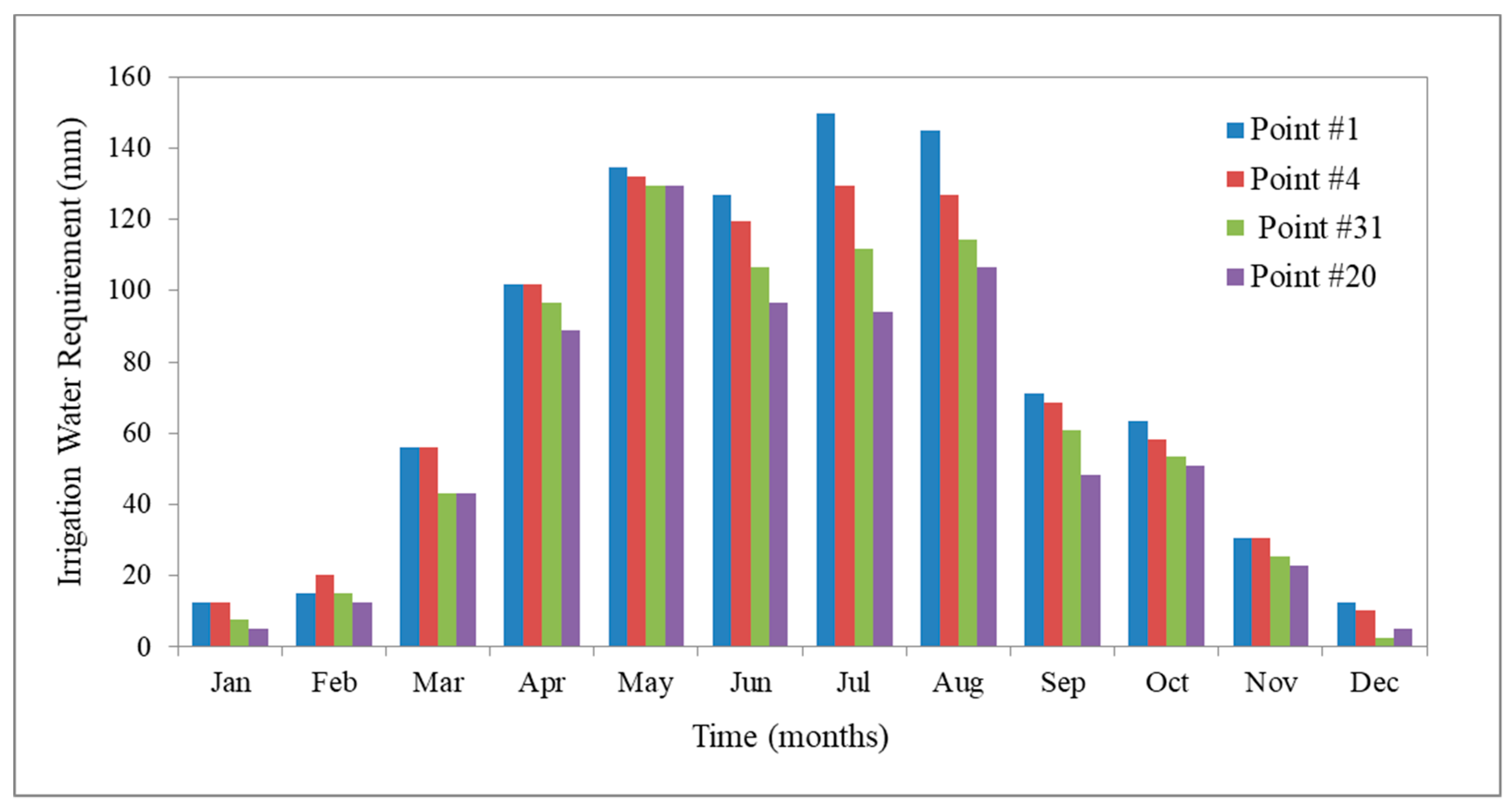
The monthly IWRs for four different chosen locations across the county during the May–August period were 10 to 14 times higher than those during the December–February period of the year (Figure 9). These findings concur with the weekly irrigation rates of about 19 to 25 mm reported by Cabrera et al. (2013) for summer months. Their estimates for the spring and fall are substantially less than those for the peak summer months; such estimates are close to zero during the winter months [11]. In addition to this temporal variation, IWRs decreased moving across the county from its north-west (Point #1) to its south-east corner (Point #20) as a result of higher rainfall and lower reference evapotranspiration.
Although the land use changes across the county (open space, low intensity, medium intensity, and high intensity) did not have a significant impact on IWR, the total water volume per land use varied substantially. Table 1 shows the IWRs for developed areas of the study area. More than 55% and about 25% of the total irrigation water volumes are used by the “Developed, Low Intensity” and “Developed, Medium Intensity” land use categories, respectively. Although “Developed, High Intensity” land use represents the areas of the county where a large portion of the population lives, it only uses 6% of the total IWR, second to “Developed, Open Space” with 14% of the county’s total annual IWR.
Annually, Harris County needs 323 million m3 of fresh water for optimum irrigation of its turf grass; this requires 136 GWh of energy, and such energy emits 80,236 metric tons of carbon dioxide. Excess irrigation is a common challenge for homeowners and crop producers. In addition, over-irrigating results in wasting energy and, consequently, unnecessary carbon dioxide emission. Results illustrating the energy and carbon dioxide losses as a result of a one-inch (25.4 mm) increment in excess irrigation in IWR for turf grass are summarized in Table 2.
An average over-irrigation of 127 mm (5 inches) above the optimum IWR (783 mm) across Harris County results in wasting 52 million m3 of freshwater resources (Table 2); this is enough freshwater annually for 152,805 Houston single families, assuming the average annual water use per single-family residential connection per 340 m3 [31]. The 127 mm of excess domestic water requires 22,065 MWh of energy, which is equivalent to the monthly energy use of 5265 county residents. According to the U.S. Department of Energy, the monthly average energy use of each resident in Texas is 4.19 MWh [32]. This total excess energy use will result in 12,994 metric tons of unnecessary CO2 emission.
In order to save water and energy and to prevent unnecessary greenhouse gas emission, we need to adopt urban landscape water management practices that help consumers conserve water use, such as using native and adaptive plant materials, optimum irrigation scheduling methods, deficit irrigation practices, or use of alternative (saline/brackish, reclaimed, and greywater) water sources.
4. Conclusions and Future Work Recommendations
Urban landscaping is a major user of Harris County’s freshwater resources. This portion of water use is expected to continue to increase as a result of the increased population growth and economic development of the county. Site-specific landscape water use data are needed to develop landscape management practices that significantly enhance freshwater conservation.
In this study, we first calculated the site-specific irrigation water requirements for turf grass across Harris County and then estimated the corresponding total energy use and CO2 emission reduction across the county if the optimum IWR is adopted. We used the IManSys model for estimation of the IWR. This model uses site-specific soil hydrological and crop water uptake parameters with long-term rainfall and evapotranspiration data to calculate the landscape optimum irrigation requirements. The results show that the estimated annual IWR of turf grass varies from 686 to 940 mm with a county average of 783 mm (323 million m3). This irrigation water requires 136 GWh of energy which emits 80,236 metric tons of carbon dioxide annually. The IWR decreases from its highest level in the north-west of the county to its lowest level in the south-east corner of the county, mainly in response to the combined effect of rainfall increase and reference evapotranspiration decrease.
Furthermore, if the annual irrigation water use is higher than the optimum water requirement by just 1 inch (25.4 mm), then the annual irrigation water loss will be 10.45 million m3, which is equivalent to annual water use for 30,561 single family houses, and its corresponding excess energy use and CO2 emission will be 4413 MWh and 2599 Metric tons, respectively. Such excess energy use would be enough to satisfy the energy needs of 1053 county residents. The findings of this work show the strong connections between optimum water management, energy use, and greenhouse gas emissions. There is a need to extend this study to other geographic locations and also to different ecosystems.
Author Contributions
Conceptualization, R.A. and A.F.; methodology, R.A. and A.F.; software, R.A. and A.F.; validation, R.A. and A.F.; formal analysis, R.A.; investigation, R.A. and A.F.; resources, R.A. and A.F.; data curation, R.A.; writing—original draft preparation, R.A., A.F. and H.H.; writing—review and editing, R.A., A.F. and H.H.; visualization, R.A. and H.H.; supervision, R.A., A.F.; project administration, R.A. and A.F.; funding acquisition, R.A. and A.F.
Funding
USDA National Institute of Food and Agriculture and Texas A&M AgriLife Research.
Acknowledgments
This work was supported by the Evans-Allen project and CBG grant no. 2017-38821-26410/project accession no. 1012198 from the USDA National Institute of Food and Agriculture and Texas A&M AgriLife Research. The authors wish to thank Devontey Lee and Yassine Cherif for their assistance in preliminary work.
Conflicts of Interest
The authors declare no conflict of interest.
References
- TWDB. Water for Texas: 2017 State Water Plan; Texas Water Development Board: Austin, TX, USA, 2017. Available online: http://www.twdb.texas.gov/waterplanning/swp/2017/doc/SWP17-Water-for-Texas.pdf?d=44485.49999995157 (accessed on 24 December 2018).
- Texas Demographic Center. 2017. Available online: http://demographics.texas.gov/Resources/publications/2017/2017_08_21_UrbanTexas.pdf (accessed on 24 December 2018).
- Electric Power Research Institute. Available online: https://www.epri.com/#/?lang=en-US (accessed on 24 December 2018).
- Diehl, T.H.; Melissa, A.H. Withdrawal and Consumption of Water by Thermoelectric Power Plants in the United States, 2010; US Geological Survey: Washington, DC, USA, 2014.
- Saidi, K.; Hammami, S. The impact of CO2 emissions and economic growth on energy consumption in 58 countries. Energy Rep. 2015, 1, 62–70. [Google Scholar] [CrossRef]
- Menyah, K.; Wolde-Rufael, Y. Energy consumption, pollutant emissions and economic growth in South Africa. Energy Econ. 2010, 32, 1374–1382. [Google Scholar] [CrossRef]
- Niu, S.; Ding, Y.; Niu, Y.; Li, Y.; Luo, G. Economic growth, energy conservation and emissions reduction: A comparative analysis based on panel data for 8 Asian-Pacific countries. Energy Policy 2011, 39, 2121–2131. [Google Scholar] [CrossRef]
- Arouri, M.E.; Youssef, A.B.; M’henni, H.; Rault, C. Energy consumption, economic growth and CO2 emissions in Middle East and North African countries. Energy Policy 2012, 45, 342–349. [Google Scholar] [CrossRef]
- Cabrera, R.I.; Wagner, K.L.; Wherley, B.; Lee, L. Urban Landscape Water Use in Texas; TWRI EM-116; Texas Water Resources Institute, Texas A&M University: College Station, TX, USA, 2013. [Google Scholar]
- Hermitte, S.M.; Mace, R.E. The Grass Is Always Greener… Outdoor Residential Water Use in Texas; Technical Note 12-01; Texas Water Development Board: Austin, TX, USA, 2012; p. 43. Available online: https://www.twdb.texas.gov/waterplanning/swp/2017/doc/SWP17-Water-for-Texas.pdf?d=10456.899999990128 (accessed on 24 December 2018).
- Cabrera, R.I.; Wagner, K.L.; Wherley, B. An evaluation of urban landscape water use in Texas. Tex. Water J. 2013, 4, 14–27. [Google Scholar]
- Hu, L.; Brunsell, N.A. The impact of temporal aggregation of land surface temperature data for surface urban heat island (SUHI) monitoring. Remote Sens. Environ. 2013, 134, 162–174. [Google Scholar] [CrossRef]
- Streutker, D.R. A remote sensing study of the urban heat island of Houston, Texas. Int. J. Remote Sens. 2002, 23, 2595–2608. [Google Scholar] [CrossRef] [Green Version]
- Global Weather Data. Available online: http://globalweather.tamu.edu/ (accessed on 24 December 2018).
- Li, X.; Wan, W.; Yu, Y.; Ren, Z. Yearly variations of the stratospheric tides seen in the CFSR reanalysis data. Adv. Space Res. 2015, 56, 1822–1832. [Google Scholar] [CrossRef]
- Tomy, T.; Sumam, K. Determining the Adequacy of CFSR Data for Rainfall-Runoff Modeling Using SWAT. Procedia Technol. 2016, 24, 309–316. [Google Scholar] [CrossRef]
- Blacutt, L.A.; Herdies, D.L.; de Gonçalves, L.G.G.; Vila, D.A.; Andrade, M. Precipitation comparison for the CFSR, MERRA, TRMM3B42 and Combined Scheme datasets in Bolivia. Atmos. Res. 2015, 163, 117–131. [Google Scholar] [CrossRef] [Green Version]
- Allen, R.G.; Pereira, L.S.; Raes, D.; Smith, M. Crop Evapotranspiration-Guidelines for Computing Crop Water Requirements-FAO Irrigation and Drainage Paper 56; FAO: Rome, Italy, 1998. [Google Scholar]
- Soil Survey Geographic (SSURGO) Database. Available online: https://websoilsurvey.sc.egov.usda.gov (accessed on 24 December 2018).
- Fares, A.; Fares, S. Irrigation Management System, IManSys, a user-friendly computer based water management software package. In Proceedings of the Irrigation Show and Education Conference, Orlando, FL, USA, 2 November 2012. [Google Scholar]
- Fares, A.; Awal, R.; Valenzuela, H.; Fares, S.; Johnson, A.B.; Dogan, A.; Nagata, N. Effect of Irrigation Systems and Landscape Species on Irrigation Water Requirements Simulated by the Irrigation Management System (IManSys). In Proceedings of the Irrigation Show and Education Conference, Austin, TX, USA, 4–8 November 2013. [Google Scholar]
- Fares, A.; Awal, R.; Fares, S.; Johnson, A.; Valenzuela, H. Irrigation Water Requirements for Seed Corn and Coffee under Potential Climate Change Scenarios. J. Water Clim. Chang. 2015, 7, 39–51. [Google Scholar] [CrossRef]
- Fares, A.; Bayabil, H.K.; Zekri, M.; de Mattos, D.; Awal, R. Potential climate change impacts on citrus water requirement across major producing areas in the world. J. Water Clim. Chang. 2017, 8, 576–592. [Google Scholar] [CrossRef] [Green Version]
- Fares, A. Water Management Software to Estimate Crop Irrigation Requirements for Consumptive Use Permitting in Hawaii Version 2.0; Report for Commission on Water Resources Management; The University of Hawai’i at Māno: Honolulu, HI, USA, 2013; p. 58. [Google Scholar]
- Smajstrla, A.G.; Zazueta, F.S. Estimating Irrigation Requirements of Sprinkler Irrigated Container Nurseries. Proc. Fla. State Hort. Soc. 1987, 100, 343–348. [Google Scholar]
- Smajstrla, A.G.; Zazueta, F.S. Simulation of irrigation requirements of Florida agronomic crops. Soil Crop Sci. Soc. Florida Proc. 1988, 47, 78–82. [Google Scholar]
- EPA. Strategies for Saving Energy at Public Water Systems. EPA 816-F-13-004; 2013. Available online: https://www.epa.gov/sites/production/files/2015-04/documents/epa816f13004.pdf (accessed on 24 December 2018).
- ERCOT. 2015. Available online: http://www.ercot.com/content/wcm/lists/114739/ERCOT_Quick_Facts_22317.pdf (accessed on 24 December 2018).
- Sovacool, B.K. Valuing the greenhouse gas emissions from nuclear power: A critical survey. Energy Policy 2008, 36, 2950–2963. [Google Scholar] [CrossRef]
- U.S. Energy Information Administration (USEIA). Available online: https://www.eia.gov/ (accessed on 24 December 2018).
- Texas Water Development Board (TWRD). Water Use of Texas Water Utilities, A Biennial Report to the 84th Texas Legislature. January 2015. Available online: http://www.twdb.texas.gov/publications/reports/special_legislative_reports/doc/2014_WaterUseOfTexasWaterUtilities.pdf (accessed on 24 December 2018).
- U.S. Department of Energy. Available online: https://www.energy.gov/articles/how-much-do-you-consume (accessed on 24 December 2018).
Figure 1.
(a) Map of the study area Harris County, Texas; (b) elevation map of the study area.

Figure 2.
Spatial distributions of long-term annual (a) rainfall and (b) reference evapotranspiration across Harris County, Texas.
Figure 2.
Spatial distributions of long-term annual (a) rainfall and (b) reference evapotranspiration across Harris County, Texas.

Figure 3.
(a) Land cover map across Harris County; (b) developed open space; (c) developed low intensity; (d) developed medium intensity; (e) developed high intensity.
Figure 3.
(a) Land cover map across Harris County; (b) developed open space; (c) developed low intensity; (d) developed medium intensity; (e) developed high intensity.
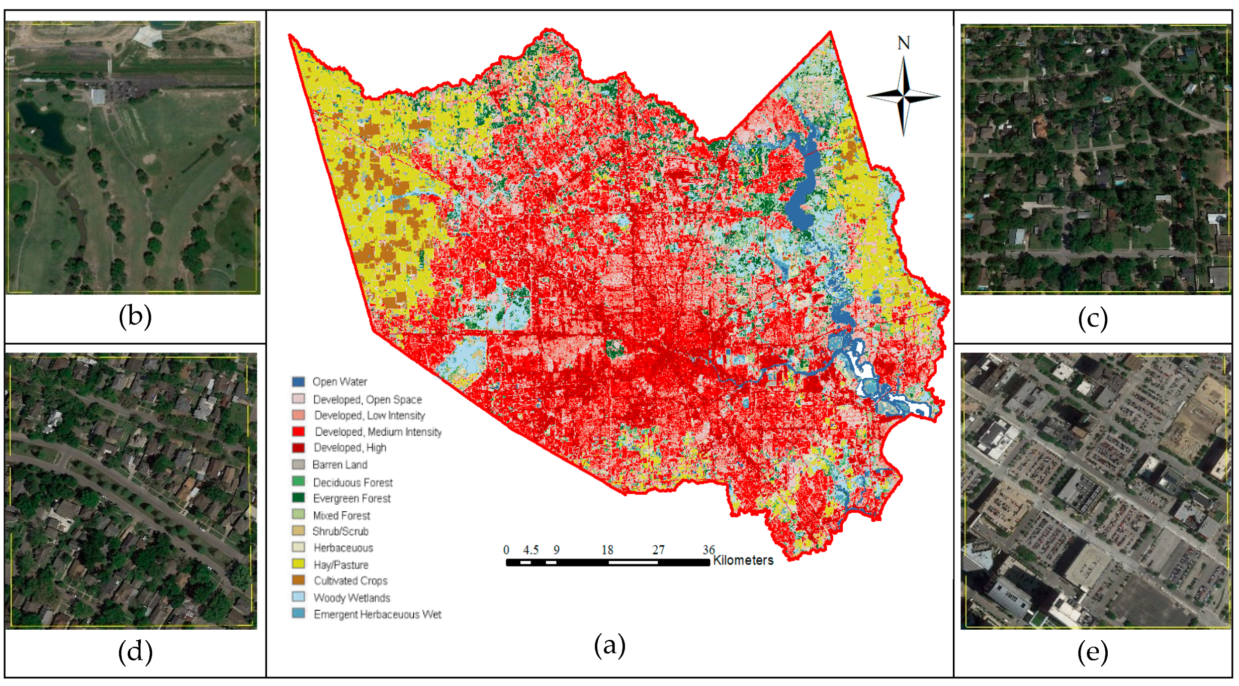
Figure 4.
A flow chart showing a summary of the overall analysis using the IManSys model.

Figure 5.
Forty-eight locations selected for simulation of irrigation requirements of turf grass across Harris County.
Figure 5.
Forty-eight locations selected for simulation of irrigation requirements of turf grass across Harris County.
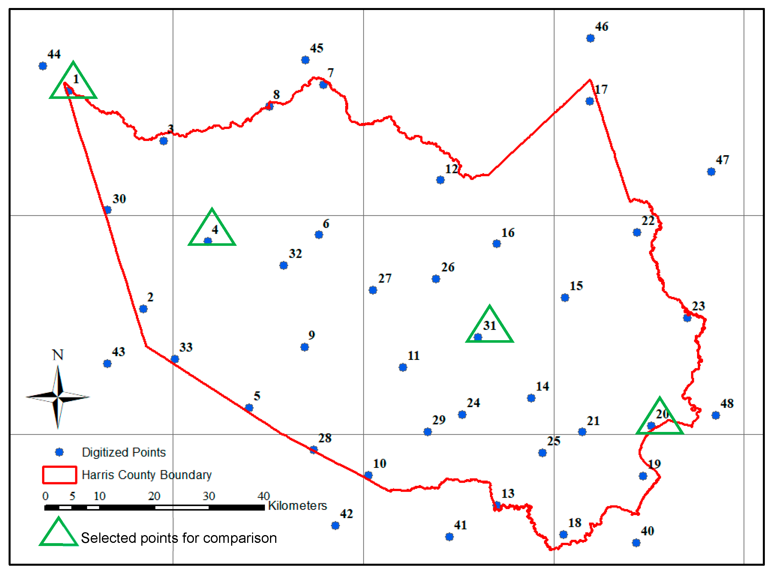
Figure 6.
A comparison chart of water budget components for four locations across Harris County.
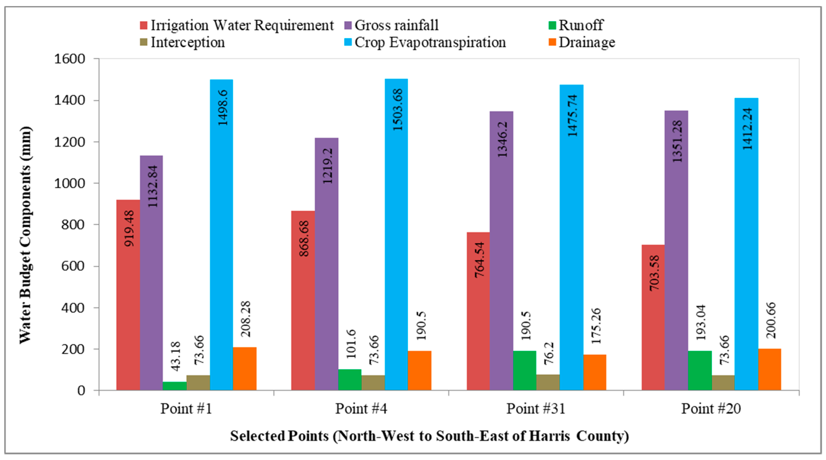
Figure 7.
Spatial interpolation of the annual irrigation water requirement (IWR) across the county.
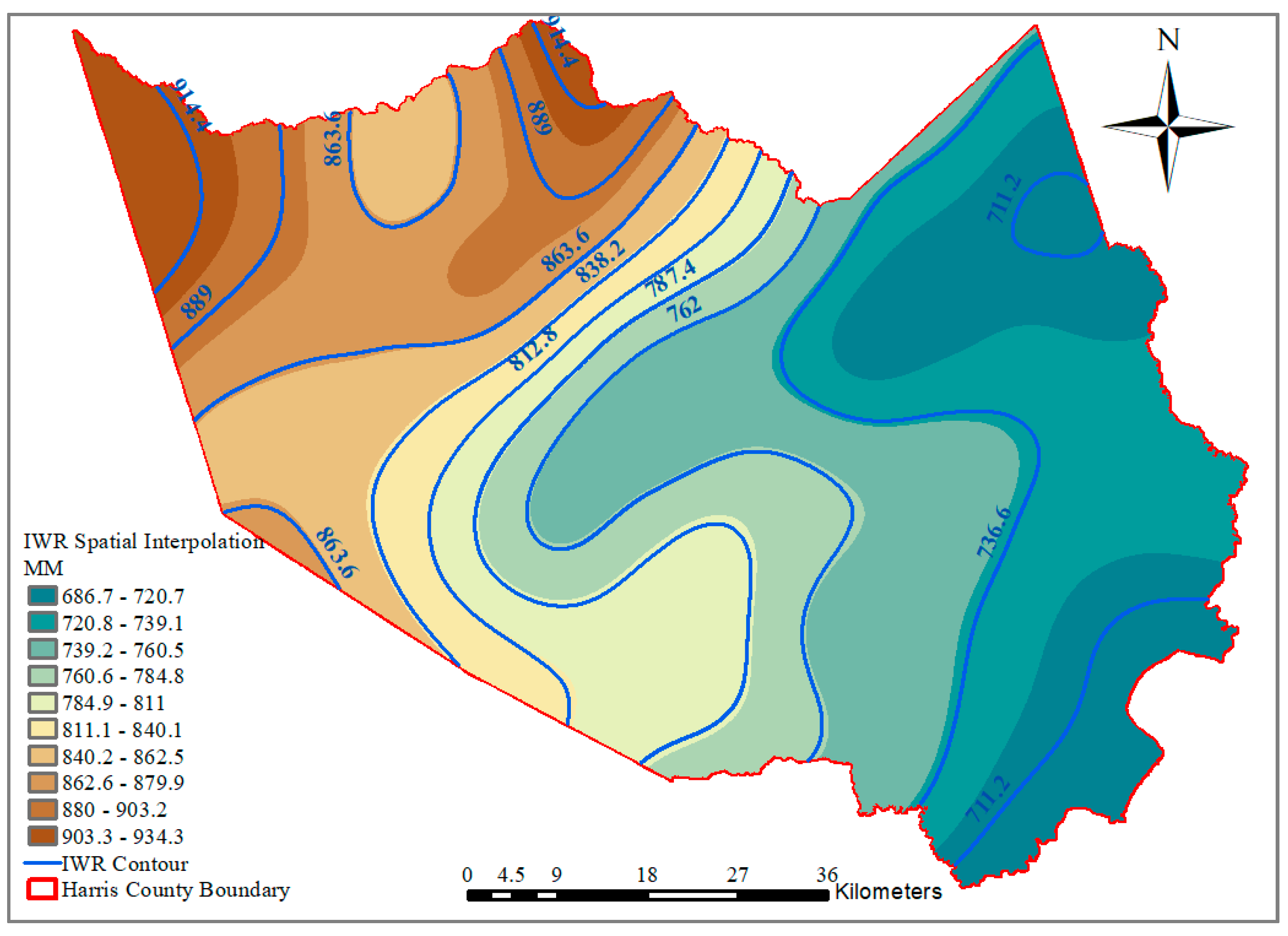
Figure 8.
Spatial interpolation of annual surface runoff across the county.

Figure 9.
Monthly irrigation water requirement (IWR) for the four selected locations across Harris County.
Figure 9.
Monthly irrigation water requirement (IWR) for the four selected locations across Harris County.

Table 1.
Irrigation water requirements for developed areas of Harris County.
| Land Cover | Total Area (km2) | Estimated Irrigated Area (%) | Annual Average IWR (mm) | Annual Average IWR (million m3) | Annual Average IWR(%) |
|---|---|---|---|---|---|
| Developed, Open Space | 592 | 10 | 783 | 46 | 14.3 |
| Developed, Low Intensity | 760 | 30 | 783 | 179 | 55.5 |
| Developed, Medium Intensity | 1007 | 10 | 789 | 79 | 24.6 |
| Developed, High Intensity | 467 | 5 | 776 | 18 | 5.6 |
| Total | 2827 | - | - | 323 | - |
Table 2.
Incremental increase in the annual IWR and the corresponding water volume, energy, and CO2 emission.
Table 2.
Incremental increase in the annual IWR and the corresponding water volume, energy, and CO2 emission.
| Annual Average IWR (Water Depth) | Annual Average IWR (Water Volume) | Annual Increase (Water Volume) | Ground Water (33%) | Surface Water (67%) | Energy for Ground Water | Energy for Surface Water | Total Energy | Total CO2 |
|---|---|---|---|---|---|---|---|---|
| (mm) | (M m3) | (M m3) | (M m3) | (M m3) | MWh | MWh | MWh | Metric Ton |
| 783 | 323 | Optimum IWR for Turf Grass (developed areas, Harris County) | ||||||
| 808 | 333 | 10 | 3 | 7 | 1639 | 2774 | 4413 | 2599 |
| 834 | 343 | 21 | 7 | 14 | 3279 | 5547 | 8826 | 5198 |
| 859 | 354 | 31 | 10 | 21 | 4918 | 8321 | 13,239 | 7796 |
| 884 | 364 | 42 | 14 | 28 | 6558 | 11,095 | 17,652 | 10,395 |
| 910 | 375 | 52 | 17 | 35 | 8197 | 13,869 | 22,065 | 12,994 |
© 2019 by the authors. Licensee MDPI, Basel, Switzerland. This article is an open access article distributed under the terms and conditions of the Creative Commons Attribution (CC BY) license (http://creativecommons.org/licenses/by/4.0/).
Share and Cite
MDPI and ACS Style
Awal, R.; Fares, A.; Habibi, H. Optimum Turf Grass Irrigation Requirements and Corresponding Water- Energy-CO2 Nexus across Harris County, Texas. Sustainability 2019, 11, 1440. https://doi.org/10.3390/su11051440
AMA Style
Awal R, Fares A, Habibi H. Optimum Turf Grass Irrigation Requirements and Corresponding Water- Energy-CO2 Nexus across Harris County, Texas. Sustainability. 2019; 11(5):1440. https://doi.org/10.3390/su11051440
Chicago/Turabian StyleAwal, Ripendra, Ali Fares, and Hamideh Habibi. 2019. "Optimum Turf Grass Irrigation Requirements and Corresponding Water- Energy-CO2 Nexus across Harris County, Texas" Sustainability 11, no. 5: 1440. https://doi.org/10.3390/su11051440
Note that from the first issue of 2016, this journal uses article numbers instead of page numbers. See further details here.