Improved Predictive Control for an Asymmetric Multilevel Converter for Photovoltaic Energy


1
Engineering Systems Doctoral Program, Faculty of Engineering, University of Talca, Curicó 3344158, Chile
2
Department of Electrical Engineering, Faculty of Engineering, Universidad de Talca, Curicó 3344158, Chile
*
Author to whom correspondence should be addressed.
†
These authors contributed equally to this work.
‡
Current address: Faculty of Engineering, Universidad de Talca, Merced 437, Curicó.
Sustainability 2020, 12(15), 6204; https://doi.org/10.3390/su12156204
Submission received: 7 June 2020
/
Revised: 21 July 2020
/
Accepted: 23 July 2020
/
Published: 1 August 2020
(This article belongs to the Special Issue Photovoltaic Power)
Abstract
:This article proposes a 27-level asymmetric cascade H-bridge multilevel topology for photovoltaic applications, which considers a predictive control strategy that allows minimization of the commutations of the converter. This proposal ensures a highly sinusoidal and stable photovoltaic injection when there are solar irradiance disturbances, generating a low distortion in the current waveform and low switching losses. To validate the performance of the control and the proposed topology, the dynamic model of the alternating current (AC) and direct current (DC) side system is first obtained, which is checked by computational simulations. Subsequently, the implementation of a master–slave control is carried out, focused on the control of DC voltage and AC current. The proposal is simulated, and the total harmonic distortion (THD) is obtained in the voltage and current waveforms. Undesired commutations, typical of the predictive control, are eliminated in the AC voltage waveform, and a proper DC voltage tracking is achieved for the high-power cell. In order to demonstrate the performance of the proposed control strategy, a low-power proof-of-concept prototype is implemented, in which the energy is injected to the grid, under the event of solar irradiance disturbances (with DC control).Then, the undesired switching in the main cell is eliminated, generating THDs in the voltage and current signal of 7.76% and 2.65%, respectively.
1. Introduction
In the global context at the end of 2019, global generation capacity from renewable sources increased by 176 GW and reached 2537 GW worldwide, which represents an annual growth of 7.4%, the average of seven consecutive years [1].
Moreover, it is expected that wind and solar power will account for 96% of the total power supply of renewable energy sources by 2050 [2]. This opens up great opportunities for power electronics, which have to efficiently integrate renewable energy into the different electricity networks and also to guarantee the quality and stability of them, especially in energies as vulnerable to disturbances as photovoltaic technology, the operation of which may require monitoring [3] and adaptive control to deal with the radiation intermittency.
Power electronics is a multidisciplinary area that plays a fundamental and mandatory role in the incorporation of photovoltaic energy technology into electrical systems. In this scenario, the neutral point clamped (NPC) converters, cascade H-bridge (CHB), and modular multilevel converters (MMC) stand out for their wide range of applications at the industry level [4,5,6,7]; they are very attractive due to the high quality of their output signals, as well as their low number of components and high power ranges [4]. The use of asymmetric multilevel topologies allows the further increase of the quality of the output signals of the converters (in contrast to the symmetric topology) subject to the ratio among the direct current (DC) sources [8,9]. Although there are several asymmetries for these converters [10,11]—and studies have addressed the different ratios among the asymmetries—it has been proven there that the proportion with the lowest harmonic component at the output of the converter is 9:3:1 [8,9]. Consequently, in this work, this ratio is used for an asymmetric multilevel converter for photovoltaic applications, which is capable of achieving a 27-level waveform.
The modulation techniques for these converters may be of several types. Some developments apply PWM (Pulse Width Modulation), SVM (Space Vector Modulation), MPC (Modulated Model Predictive Control), SHE (Selective Harmonic Elimination), and Staircase Modulation [4,6,9,12,13,14,15,16,17,18,19,20]. Similarly, there is a wide variety of control strategies that can be applied to multilevel converters. Among them, there are linear strategies, such as PI (Proportional Integrative) and PR (Proportional Resonant) [20,21]. Additionally, nonlinear strategies, such as hysteresis control, predictive control, and fuzzy control, can also be applied [22,23,24]. Particularly, the predictive control strategy is suitable for multi-variable control in DC/DC and DC/alternating current (AC) converters. For asymmetric multilevel converters, predictive control has important advantages because the computational cost is considerably reduced, as it eliminates the redundant states for the 9:3:1 configuration, leaving only 27 valid states. Thus, the events of commutation can be bounded, significantly reducing the computational burden [25]. Indeed, for asymmetric multilevel topologies, the algorithm has a maximum of 27 iterations, in which the cost function is evaluated and the valid state that minimizes that function is obtained. For comparison, the symmetric counterpart considers levels, where N represents the number of H-bridge cells of the topology. Considering this, it is observed that to obtain the 27 levels, the symmetric converter requires valid states (considering four states per cell). Because of the latter, the predictive algorithm would have a greater computational burden when evaluating valid states as compared to the 27 valid states of the asymmetric version. Subsequently, this lower computational effort makes the predictive control a feasible solution for asymmetric multilevel topologies.
Although this strategy has been well studied by the scientific community [23,26], with developments of various applications for multilevel converters [27,28], it is still possible to find new improvements in both its optimization and its application to multi-variable systems. Thus, this article aims to optimize the application of predictive control in multilevel topologies, reducing undesired commutations in the high-power cell, to avoid switching losses. Hence, this work aims to develop an asymmetric multilevel converter to inject photovoltaic energy and to guarantee power quality considering solar irradiance changes falling upon the photovoltaic arrays, minimizing the commutation of the high-power cell. For this, a 27-level asymmetric multilevel converter with a 9:3:1 ratio is proposed, commanded by a predictive control strategy that optimizes its switching. Simulated and experimental results are presented in order to validate the proposal.
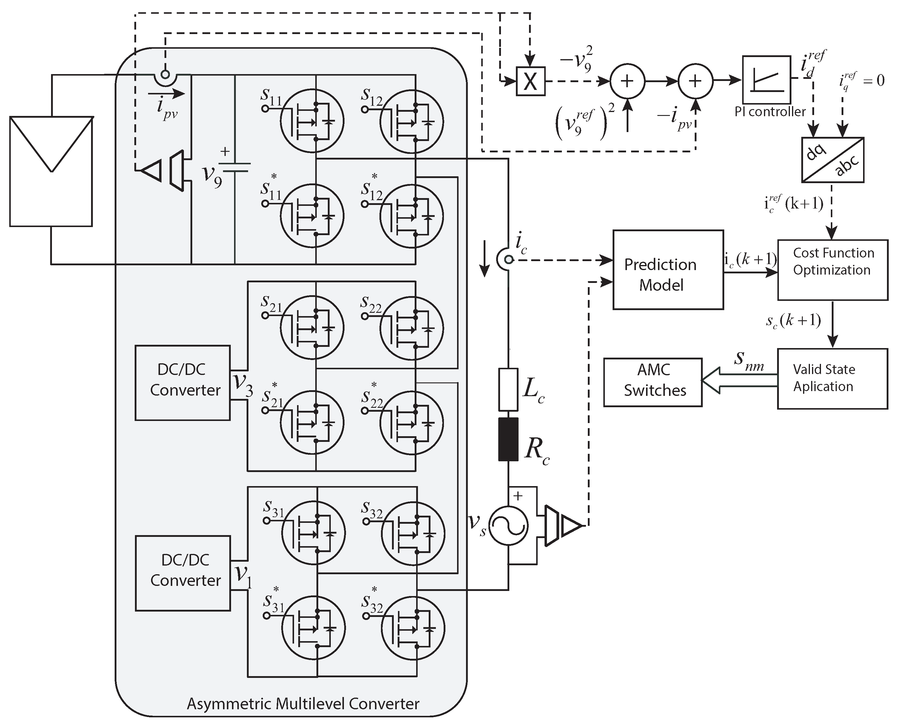
The topology developed in this work has several characteristics: Highly sinusoidal voltage signal, redundant state elimination, and low commutation frequency. Additionally, this topology needs to connect each of its stages to independent DC sources. The latter makes this type of power converter very adequate for photovoltaic systems, as it can be distributed in such a way that each stage can be connected to a different photovoltaic string. This permits avoidance of the use of galvanic isolation. However, the main disadvantage of this topology is its low modularity because the signal quality of the converter depends on compliance with the 9:3:1 ratio. Therefore, at the time of a failure in the high-power cell (HPC) or in the medium-power cell (MPC), the output signal will suffer from significant distortion, which can result in significant harmonic injection to the power grid. The developed topology of the 27-level asymmetric multilevel for photovoltaic energy injection into the power grid is shown in Figure 1. There, it is possible to observe that is composed of three single-phase cells: A high-power cell (HPC), medium-power cell (MPC), and low-power cell (LPC) connected in cascade. Each cell considers the use of photovoltaic panels with different levels of DC voltage under the ratio 9:3:1. It is possible to find in the literature other asymmetry proportions for this converter [29,30]; however, it has been shown that the used relation minimizes the redundant states [8,9] and, therefore, generates less harmonic content in the resulting waveforms of the converter. Due to the asymmetric distribution of the voltages, HPC handles, at most, one of the total power of the converter, while the rest is distributed between the MPC and LPC modules. These last two cells have to ensure the proportion in terms of the DC voltage of the HPC cell despite the changes in solar irradiance upon the photovoltaic panels. It is important to mention that the voltage ratio for the MPC and the LPC must be ensured by external control loops and additional hardware (DC/DC converters), as deeply explained in [31,32]. It is important to consider that non-compliance with asymmetry implies a harmonic distortion in the output signal of the converter, which means losses attributed to the generation of harmonics in the AC current.
2. The Proposed Solution
2.1. Converter Modulation
To understand the modulation of the converter, it is necessary to identify its valid states. For a three-cell topology of a CHB converter, there are 64 valid states, and 37 of these are redundant ‘zero’ states. It is not possible to use these redundant states for a purpose other than the equitable alternation of losses between the semiconductors of the converter cells, since these do not influence the output signal of the converter. Thus, only two matrices of 27 valid states will be used, where the first matrix will consider the zero states ‘11’ and the second matrix will consider the zero states ‘00’. In Section 2.5, this topic will be addressed in greater detail, which has as its main objective the equitable distribution of the zero states in each cell in order to distribute the conduction losses of the semiconductors of the three equitable cells. The generalized valid states for this converter are shown in Table 1, where the marked framed states are those that present undesired commutation generated by the standard predictive control. This issue is widely developed in later sections.
2.2. AC Link Dynamic Model
To formalize the behavior of the converter, it is necessary to obtain the dynamic model of the system. For this, the following equations are defined as follows:
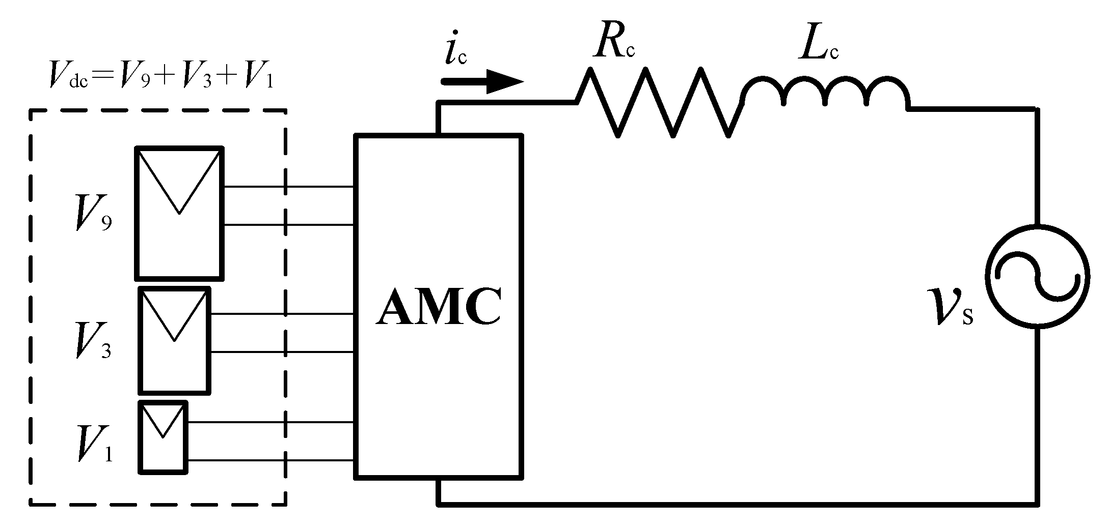
where is the virtual DC voltage of the converter that is composed by (DC voltage of the HPC), (DC voltage of the MPC), and (DC voltage of the LPC). The converter voltage can be expressed as
where represents the AC voltage of the converter and is the switching function that represents the 27 valid non-redundant states of the converter.
Similarly, can be represented by the sum of the AC signals of each cell.
where , , and correspond to the AC voltage of the HPC, MPC, and LPC, respectively. The following dynamic equation of the converter is obtained with the help of the simplified circuit of Figure 2.
Once the dynamic model of the converter is obtained, it is necessary to find its discrete equivalent [33]. This is required to program the predictive algorithm and to be able to evaluate each valid state of the converter discretely.
For this, a first-order Euler approximation is applied in the derivative of the dynamic Equation (4).
where corresponds to sampling time.
Reordering the Equation (5), predicted current can be obtained.
Finally, Equation (6) predicts the future state of the converter current.
2.3. DC Link Dynamic Model
Additionally, it is necessary to formalize the DC link behavior of the HPC in order to apply the master control loop. For this, a power balance between the converter and the HPC capacitor is considered.
Equation (7) represents the power balance between the AC side of the converter and the DC side capacitor, where represents the capacitor voltage, which is also represented by . Applying the Laplace transform to Equation (7) and considering the term as a disturbance:
where s represents the Laplace term. From Equation (8), the system transfer function is obtained, which is represented by Equation (9).
From the function, the calculation of parameters of the corresponding PI control loop was performed. Using classic control tools, such as Root Locus, a settling time of 2 s, with no overshoot in the step response, was established; it resulted in 0.00040292 and 0.0001477.
2.4. Predictive Algorithm
The diagram in Figure 3 shows each of the steps to implementing the predictive control. First, a measurement stage is observed, in which the converter current and the grid voltage are obtained. Then, in the second stage, the optimal switching state that was obtained in the previous prediction cycle is applied. After this, the equation evaluation process (6) is initialized. This process is repeated 27 times, which corresponds to the number of valid states considered in the converter. Once is obtained, the cost function is calculated, whose value depends on the absolute difference between and . The value of this cost function is then optimized, considering the valid state that generates its minimum value. Finally, the optimal valid state is stored to be applied in the next control cycle.
2.4.1. Stability and Robustness Assessment
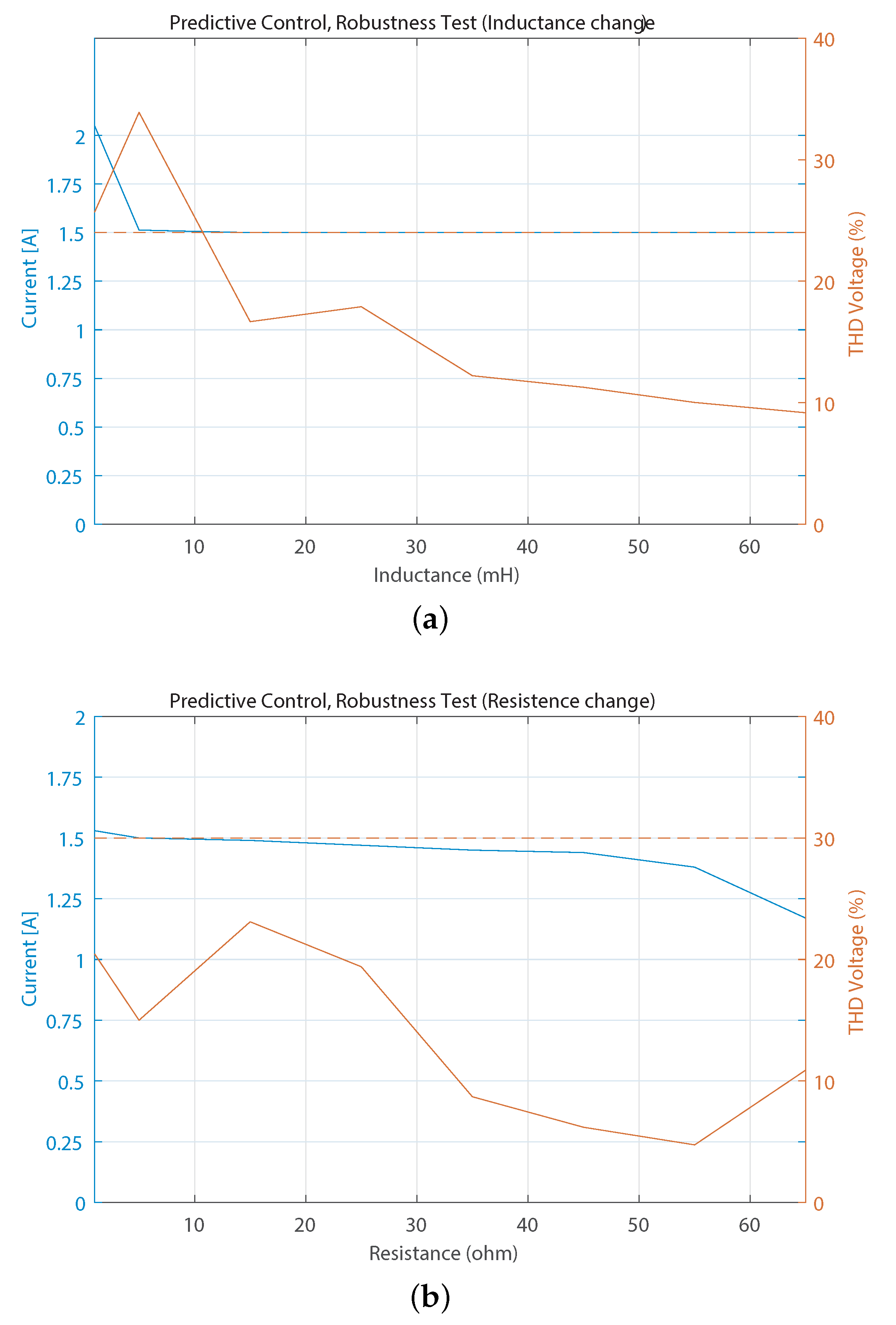
To demonstrate the robustness of the proposed predictive control, the simulation is carried out, considering the AMC converter and the control strategy under study (see Figure 3). Within the simulation, changes were made in the system parameters: The inductance and resistance of the converter were varied in a certain range in order to analyze the behavior of the control. The parameters considered in the simulation are shown in Table 2. On the other hand, the Figure 4a,b represents the response of the closed-loop system to the variation of inductance and resistance of the converter, respectively. For both figures, the left and right axes represent the converter current and the total harmonic distortion (THD) of the voltage, respectively. It is also possible to observe a segmented line, which represents the current reference of the converter.
Initially, the nominal values of resistance and inductance of the converter are 5 Ω and 20 mH, respectively. It is observed that when applying an inductive change (see Figure 4a), the system does not present big variations in the current signal of the converter (compared to its reference). Indeed, the current is kept constant with the change of this parameter, and the THD remains low. However, if the value of the inductance continues to increase, a significant distortion in the dynamics of the current of the converter is naturally expected.
In Figure 4b, it can be seen that when there is a resistive change, the precision of the predictive control is reduced. Indeed, when increasing or decreasing the resistive load, the control gradually moves away from its reference. However, within a range of of the load, the control loop still can achieve an acceptable behavior because the converter voltage keeps its sinusoidal shape.
On the other hand, in the predictive control, it is not possible to carry out a stability analysis using conventional methods. However, there are studies that establish some methods to guarantee asymptotic stability in a closed loop. Those methods are “Continuity of system and cost”, “Uniform weak controllability”, and “Properties of constraint set”, among others [34].
2.4.2. Mitigation of Undesired Commutations
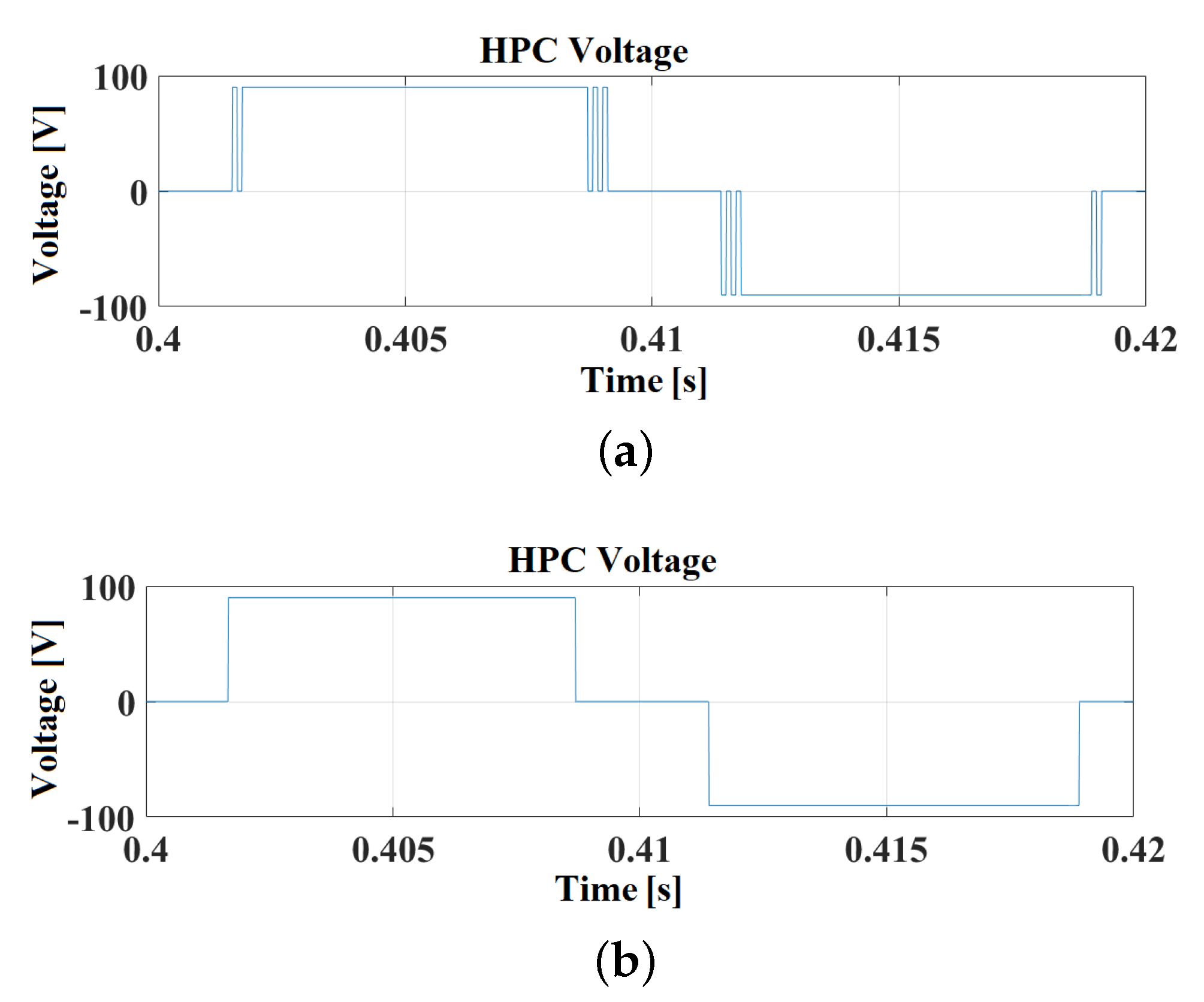
Following the steps in the diagram of Figure 3, a correct control of the converter current was achieved. Nevertheless, several commutations were observed in the changes of states of the cells. According to the nature of the converter, it was determined that such commutations have a negative effect, particularly on the HPC (Figure 5a), since it manipulates the highest amount of power (maximum ), whereby additional switching losses would be generated in terms of the expected signal (see Figure 5b). Although the same effect also occurs in the MPC and LPC, they handle much lower power than the HPC, so they are not considered in the present study. The effect produced by additional commutations is normal in predictive loops, especially if it does not have a penalization element of commutations in its cost function. Given the latter and to overcome this problem for the HPC, it is proposed to establish a matrix of penalties (based on a method addressed in article [35]) that limits the additional commutations produced in the changes of state of the HPC. Therefore, a new term is applied in the cost function, which serves as a restriction that acts to eliminate these undesired commutations. This term is a matrix whose values are based on the present state k and the future state . After applying this matrix of restrictions in the cost function of the predictive control, it is expected to obtain a signal similar to Figure 5b.
To perform the constraint matrix, it is necessary to consider the valid states of the Table 1. There, it can be seen that the framed states are those that generate the commutations in the HPC. Considering the latter, the constraint matrix described in Table 3 is generated, which is applied as a new component in the cost function .
Table 3 is obtained from Table 1 and consists of 27 rows and 27 columns, whose rows represent the current valid state and whose columns represent the future valid state . Table 3 shows the commutation regions based on the present and future states previously mentioned, where ’1’ represents commutation between the states and ‘0’ the non-commutation between them. The logic of Table 3 is to position itself in the current state and determine if the future state commutates the HPC. It is expected that, at the time that an undesired commutation happens, the cost function will increase its value, preventing the application of the respective future state unless there is really a change in the HPC and the converter enters within the non-commutation region. This method ensures the reduction of commutation efficiently in the HPC. Considering the above, the new cost function is as follows:
where corresponds to the cost function and is the constraint matrix shown in Table 3, k is the present time, is the state to be evaluated, and corresponds to the weighting factor that is calculated based on the maximum permissible error in the cost function to be obtained.
2.5. Zero State Equalization
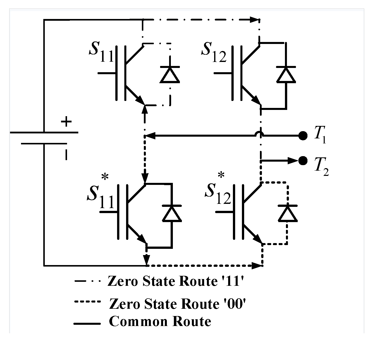
In order to get the most out of the proposed topology, it is necessary to strategically use the zero states of the converter in order to distribute the load equally in the semiconductors and avoid their partial use. A basic scheme of the H-bridge cell is shown in Figure 6, where the zero state ‘11’ is observed, which implies that both and are closed. This indicates that the cell does not deliver voltage. However, it allows the current to pass through an eventual load at terminals and . It is worth mentioning that the switches and have a phase shift of with respect to and .
If only the zero state ‘11’ is used, the semiconductors and would suffer a greater loading as compared to the semiconductors and , which would produce an imbalance in their lifetimes. It is important to clarify that when considering two zero states per cell, and not only one, there is a total of valid states in the topology. However, the existing redundant states are only zero states, which do not contribute in the amplitude of the signal at the output of the converter. The proposed technique will take advantage of all the zero states in order to distribute them, i.e., each of the switches is used equally when a zero state occurs. Subsequently, a suitable way to distribute the semiconductor load equally is to alternate two state tables (created from the table with 64 valid states) in each wave cycle. In this way, this guarantees equal usage and heat distribution throughout all four switches of each cell.
2.6. Control Strategy
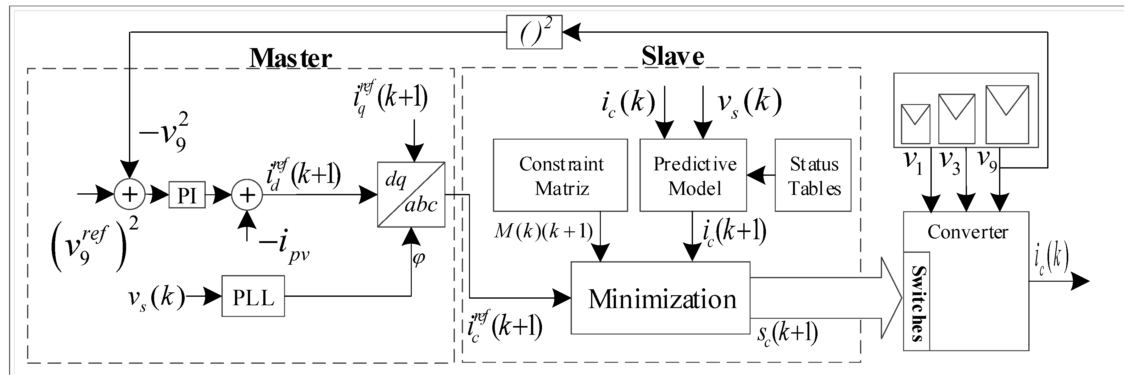
The diagram in Figure 7 shows the control proposal, which considers a master–slave approach. The master-loop corresponds to the DC control of the HPC, while the slave-loop corresponds to the current control of the AC side of the converter. The master-block is implemented through a proportional-integrative loop (PI), while the slave-block is controlled through a predictive loop.
The slave-loop is responsible for controlling the converter current in accordance with the reference of active and reactive current, and , which are provided externally, where is delivered by the master-control and is set to zero. This block aims to provide the set of valid states for the future state of the converter . Subsequently, an inverse Park-transform block is observed, which transforms the references from the plane to the plane, giving the future current reference . This signal reaches the predictive control block (described in Figure 3) in the same way as the converter current and the grid voltage.
On the other hand, a PI block is responsible for controlling the voltage in the HPC of the converter, which is fed with the difference between the signals and , taking into account the transfer function described in Equation (9). The output of this PI block provides the direct current reference to maintain the voltage of the HPC in the reference .
3. Simulation Results
This section shows and discusses the main waveforms obtained with the methods presented in this proposal. This work was simulated in the PSIM and MATLAB softwares; solar irradiance disturbances in the photovoltaic array connected to the HPC were considered. The considered parameters are shown in Table 2.
3.1. Transient State Analysis
In this section, a dynamic analysis of the signals obtained by simulation is developed with the purpose of demonstrating the proper tracking of the current reference through the master–slave approach.
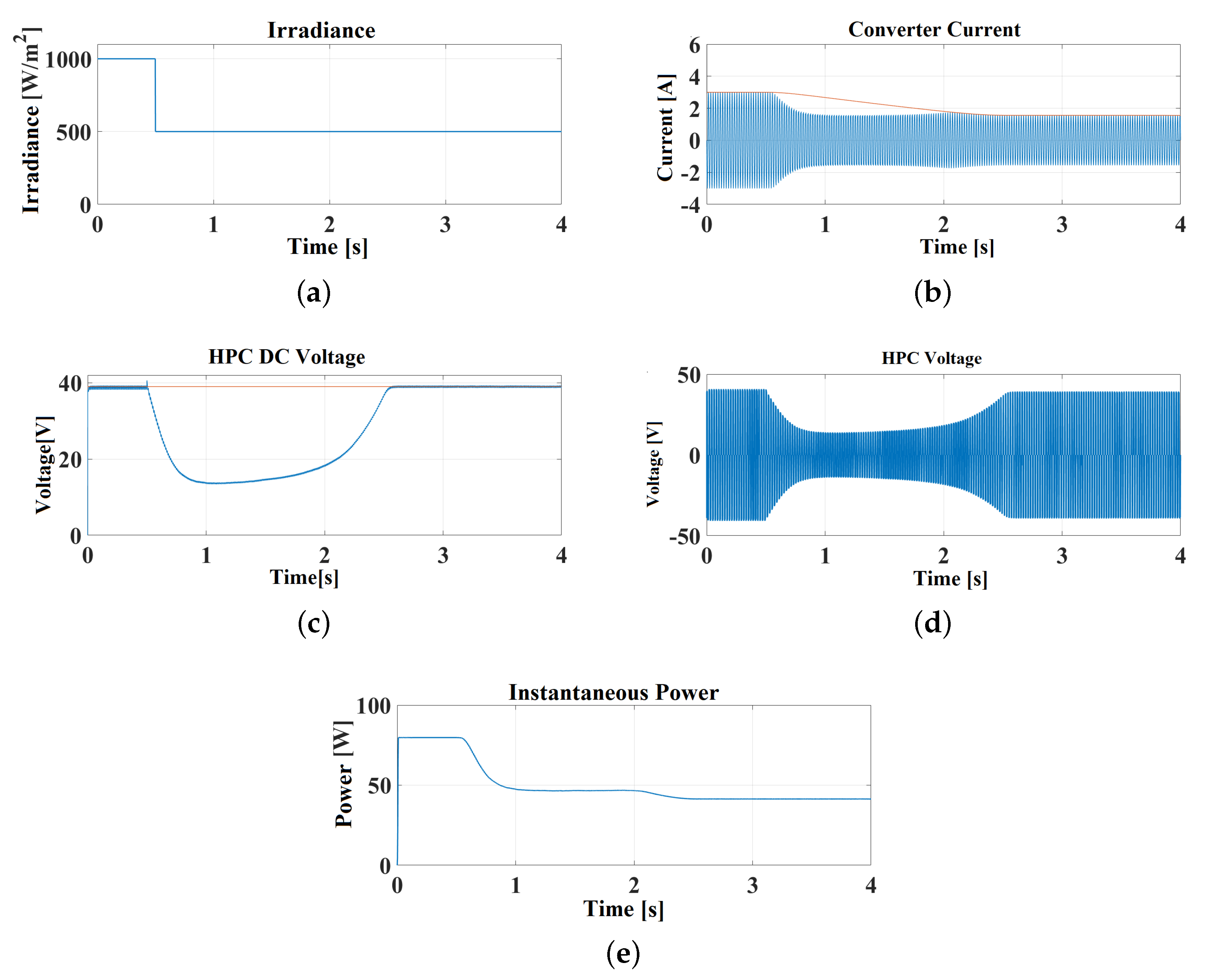
To evaluate the performance of the control strategy, an initial solar irradiance value of is imposed for the photovoltaic array of the HPC. Starting at 0.5 s, the solar irradiance is reduced to , emulating an eventual loss of generation in the photovoltaic panels due to the shading effect (see Figure 8a). Once this change in the photovoltaic generation is imposed, it can be seen in Figure 8b that the converter current at t is in a steady state at the value of . At t, the dynamic change in the photovoltaic generation takes place, and there is a drop in the current signal and the reference current (generated by the master-loop). The latter gradually descends to a final value of . This reduction occurs because the photovoltaic generation decreases and, therefore, so does the current injected into the grid. It is observed that, given the dynamic change, the current is adjusted to the new generation condition in order to ensure that the capacitor of the HPC is kept in the reference (see Figure 8c).
Although the dynamics of the predictive control in open loop are quite fast (in the order of ), in a master–slave scheme, this dynamic is governed by the slower system, which, in this case, corresponds to the voltage control of the HPC, which is carried out by a proportional-integrative control (PI) with a settlement time of and no overshoot. For this reason, the current takes to reach its reference value.
For both the DC current and the voltage, there is a higher ripple at compared to , which is due to the fact that this loop corresponds to a PI (linear control) block, which is designed for a specific operating point. Therefore, when the operating conditions change (solar irradiance disturbance), a decrease in the ripple in the response of both variables can be seen. This effect is also attributed to the fact that the new generation conditions involve manipulating a smaller amount of current.
On the other hand, Figure 8d shows the AC voltage of the HPC, which has a switched amplitude between 0 and . At t, it is observed that the voltage of this cell takes about to stabilize. Figure 8e shows the instantaneous power injected into the grid, where it can be seen that, at t , this has a steady state value of . However, that value drops to due to the decrease in the generation of the photovoltaic panels.
3.2. Steady State Analysis
In this section, the results obtained in simulation are discussed; mainly, it is intended to confirm the correct response of the system in the steady state and also to demonstrate the effective elimination of undesired commutations, which are included in the objectives of this work.
In Figure 9a, the signal obtained in the HPC is shown by applying the constraint matrix , while in Figure 9b, the signal obtained in the HPC is shown without applying the constraint matrix. It is worth mentioning that, for each wave cycle, the HPC should commutate only four times and not 16 times, as shown in Figure 9b. It is observed that with the restriction of commutations in the cost function, the commutations produced in the HPC state changes are completely eliminated. Therefore, and considering the previous figures, the commutations in the HPC are eliminated to with the help of the constraint matrix in the cost function.
The MPC and LPC in Figure 9c,d do not show changes in the event of disturbances because, for simulation purposes, the cells are fed with external DC sources in order to follow the 9:3:1 ratio. It can be seen that there are additional commutations in the changes of state of the MPC and LPC. The latter is due to the nature of the predictive control and the absence of restrictions in the cost function to mitigate them. In fact, it is established that the commutations of the smaller cells generate a negligible impact (with respect to the commutations in the HPC) on the output signal of the converter.
Figure 9e shows the converter voltage signal, where the stepped shape is observed due to the nature of the asymmetric multilevel topology 9:3:1, obtaining a maximum of 27 levels.
Figure 9f shows the converter’s current signal, where THD is obtained in the current and voltage signals of and , respectively. These values are positioned within the standards recommended by the Institute of Electrical and Electronics Engineers (IEEE) [36]. Finally, in Figure 9g, the commutation of the status tables is shown, where an equitable distribution of the zero states is ensured, which prevents unequal loading of the semiconductors of the converter.
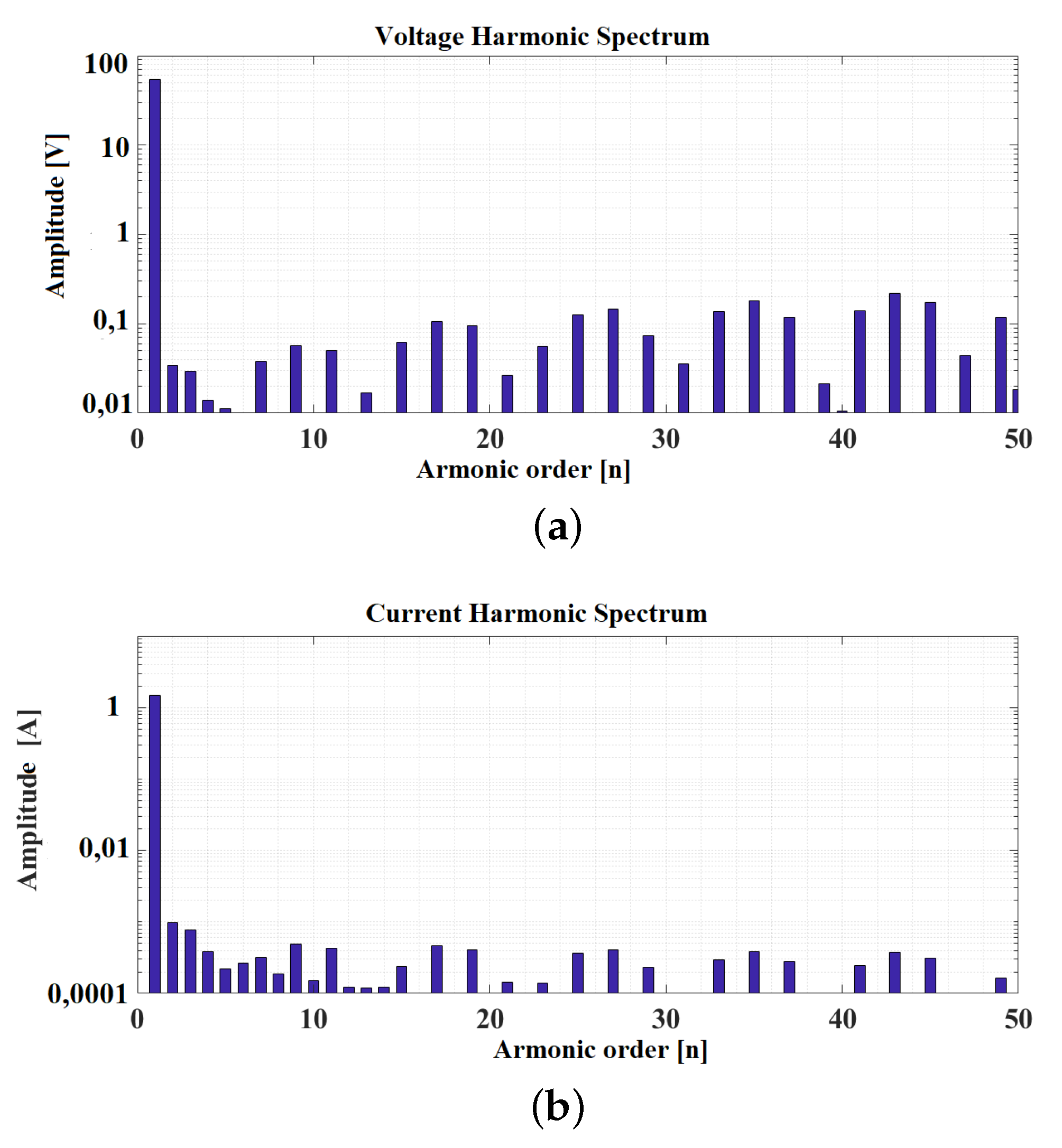
Figure 10a,b shows the harmonic spectrum of the voltage and current of the converter using predictive control, where a logarithmic scale is used on the y-axis, in order to show more clearly all the components of the spectrum. On the other hand, the x-axis represents the harmonics of the signal, which is normalized with regard to the fundamental frequency (50 Hz). Therefore, the first harmonic corresponds to the fundamental frequency; the other harmonics (from 2 to 50) are multiples of the fundamental.
It is important to mention that the harmonic voltage spectrum concentrates its greatest amplitude on the fundamental frequency. The amplitude of the rest of the harmonic components is very far from the fundamental amplitude, and can be easily eliminated with a passive filter. Figure 9a,b demonstrates the low harmonic component of this converter compared to other topologies, which is one of the main features of the asymmetric multilevel converter presented in this work.
4. Experimental Implementation
The general connection scheme is the same as that presented in Figure 1, where the asymmetric multilevel converter (AMC) is connected to the power grid in order to inject the power generated in the PV modules. The same values of the simulation are considered for the parameters in the proof-of-concept prototype.
4.1. Commutation Elimination in the HPC
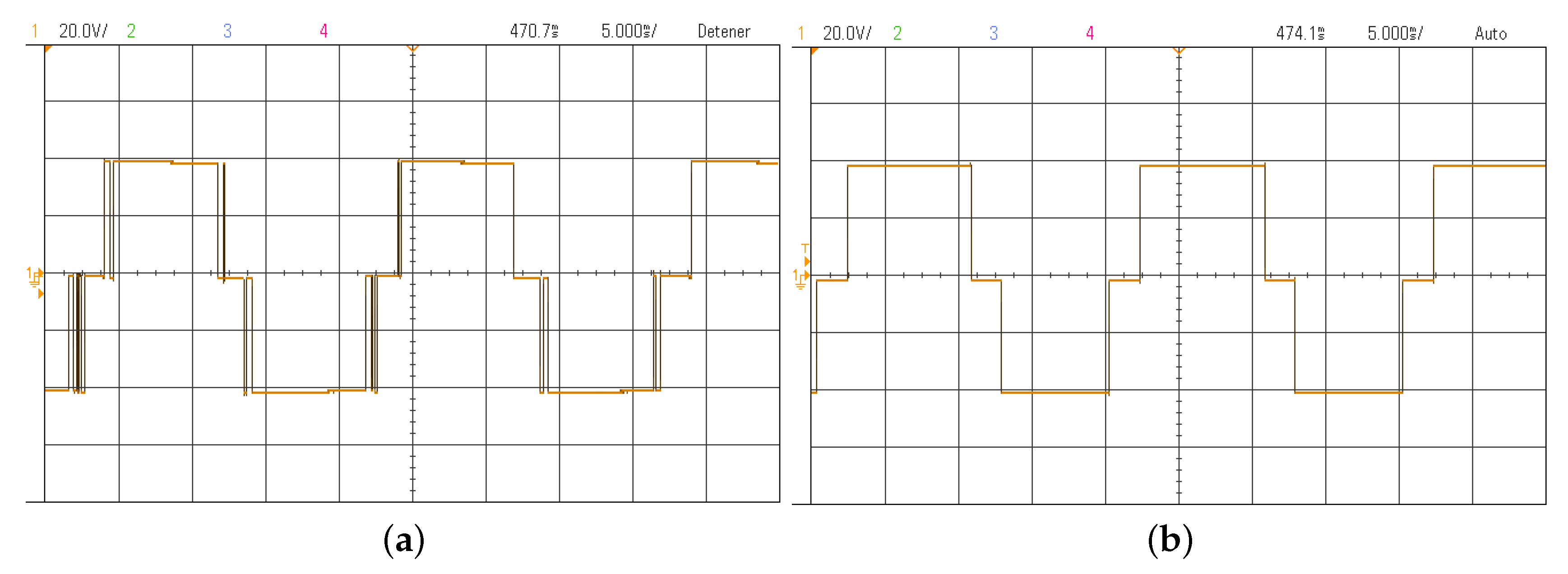
In this subsection, an experimental comparison is made between the application and the absence of the restriction table within the cost function of the predictive control applied to the AMC. The latter is to check if undesired commutations are actually being eliminated in the HPC, and to experimentally validate the results obtained in the simulation. Thus, initially, the predictive control is implemented in the converter without the incorporation of the M matrix (see Figure 11a). As a result, a voltage signal is obtained in the HPC with undesired commutations in the state changes of the cell. This result normally describes the typical behavior of a predictive control strategy where there is a change in the selection of valid states mainly reflected in the changes in the state of the HPC.
On the other hand, the matrix of switching restrictions is incorporated in order to validate the results obtained in the simulation. In Figure 11b, the results obtained by applying the M restriction matrix in the cost function of the predictive control are shown, as is the total mitigation of undesired commutations in the changes of state of the HPC. Therefore, the results obtained in the simulation can be validated.
4.2. Discrete Master Control
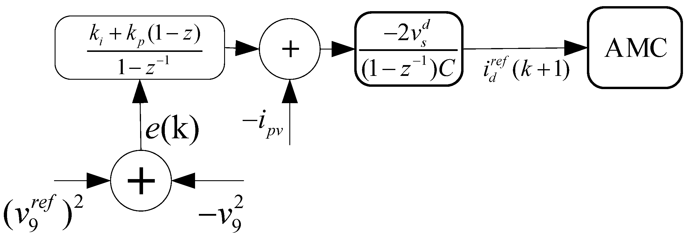
In order to introduce a linear controller, it is very important to establish the expected dynamic behavior. Figure 12 represents the master control scheme based on the power balance model shown in Equation (8), which was described in the previous sections. It has to be considered that the implementation of the control algorithm is discrete. Therefore, the control loop must be expressed in the Z plane, as shown in Figure 12. The same parameters of the simulation are used for the experimental tests.
4.3. Result Analysis
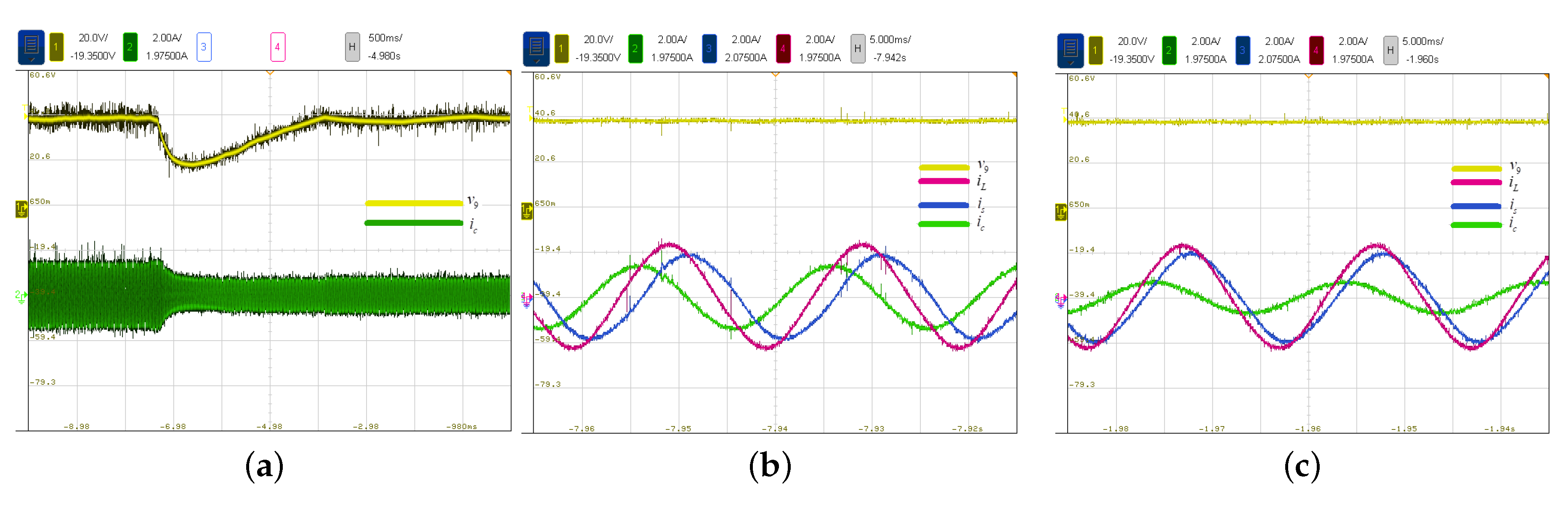
In this section, the tests and analyses of the master–slave control are carried out, where disturbances are applied in the power generation of the photovoltaic panels connected to the HPC of the converter.
For these tests, the parameters of Table 2 are considered. In Figure 13a, two signals can be seen; (channel 1) corresponds to the DC control of the HPC, which was previously tuned, establishing a settling time of without overshoot. It is possible to observe in Figure 13a that the dynamic response complies with the times established in the tuning of the controller, as previously established. In addition, the signal (channel 2) represents the behavior of the converter current, where it is observed that prior to the disturbance in the solar irradiance of the photovoltaic panels, the injection current to the grid is A. After the disturbance, the current decreases to A, since the power generation decreases under this scenario. The current is regulated (because of the master control), such that the voltage of the HPC is kept at the established reference of . It is possible to confirm that both the settling time and the overshoot in the DC voltage of the HPC behave according to the design parameters.
Additionally, two graphs are shown in Figure 13b,c. The first image represents the behavior of the currents , , and in the steady state prior to the solar irradiance disturbance. The second image represents the behavior of the same currents in the steady state after the solar irradiance disturbance. In the latter, it can be seen that the quality of the current signal injected by the converter in both operating conditions is highly sinusoidal with low THD. Current signals appear with evident noise on the experimental prototype. This is due to several factors, such as sensing errors, electromagnetic noise, losses due to length of wiring, parasitic capacitances, voltage drop in the semiconductors, and passive elements, among others. In particular, in this implementation, losses are attributed to the magnetic field generated by the inductor of the converter, some inevitable long tracks at the gate of the MOSFETs (metal oxide semiconductor field-effect transistor) of the H-bridges, the wiring between the digital signal processing (DSP) and the field-programmable gate array (FPGA), and the calibration of the sensors.
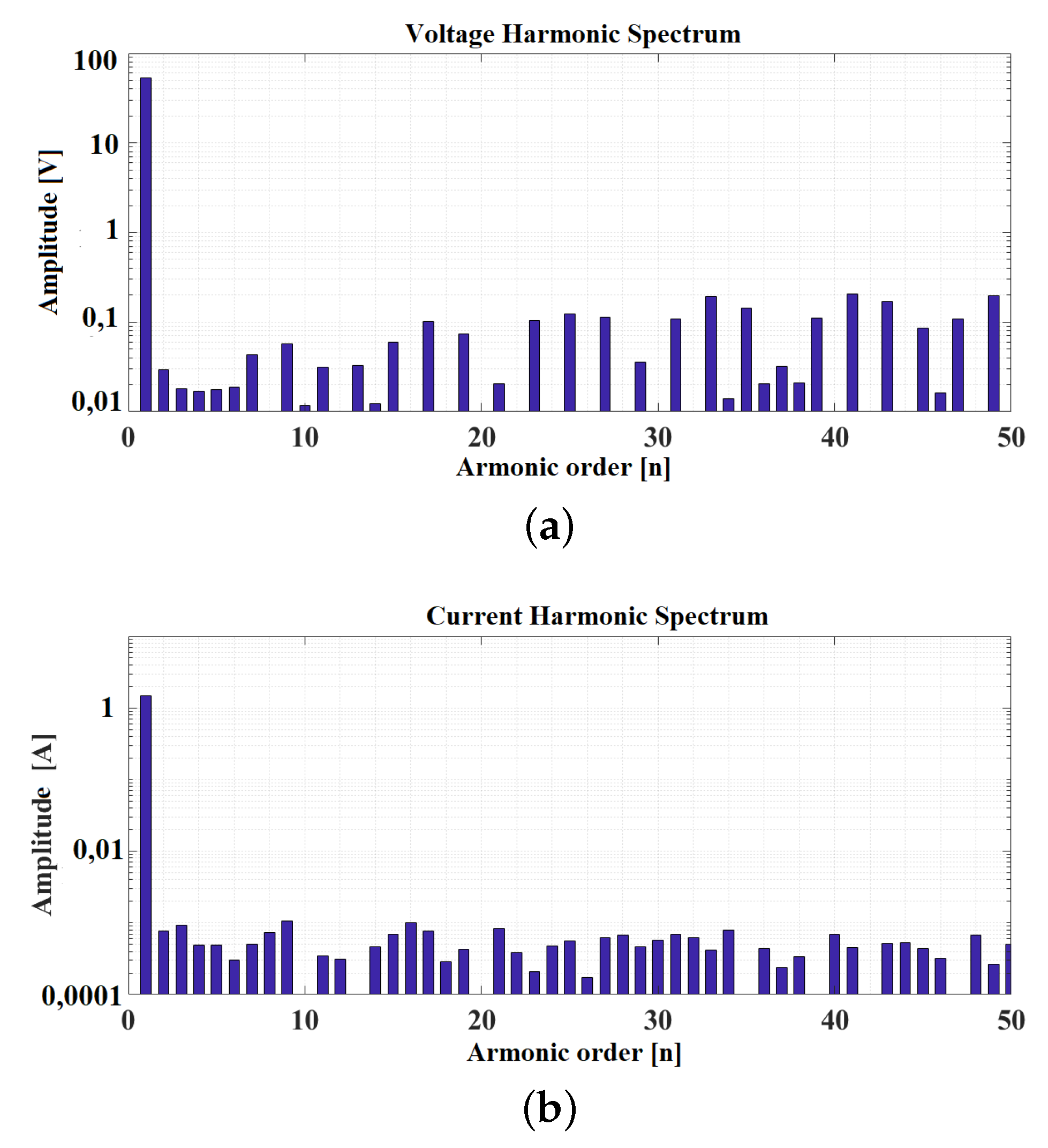
Then, the harmonic spectra obtained for the current and voltage signals of the experimental setup in the steady state are shown. The harmonic spectrum of the voltage signal of the AMC prototype is shown in Figure 14a, and indicates a similar distribution to the one obtained in the simulation, where there is the highest amplitude concentrated in the fundamental frequency. From the second harmonic onwards, the lower-order components of high frequencies (up to ) are distributed, where the second harmonic has an amplitude of the order of .
In Figure 14b, the harmonic distribution of the converter’s current signal is shown, which is a consequence of the harmonic voltage distribution and subsequent attenuation due to the inductive component of the filter . To obtain the value of the inductor capable of generating a THD lower than , the Equation (11) is considered, which was obtained following the procedure developed in [37].
where refers to the maximum switching frequency and to the maximum permissible current error.
In order to obtain the maximum switching frequency, an analysis is performed in the LPC because it switches at a higher frequency than the rest of the cells of the topology. In this analysis, a total of 50 commutations per cycle were obtained, of which 10 commutations were attributed for each edge due to the predictive control action, obtaining a total of commutations () of:
where is the total number of commutations per cycle of the LPC and corresponds to the commutations, in the LPC, provided by the nature of the predictive control. Considering that the voltages used in the low-power prototype are for the converter and for the AC source, and establishing an allowable error of for the converter current, it can be said that:
For practical reasons, there were only off-the-shelf inductors of for the prototype implementation. It should be mentioned that in the prototype, there are conditions that increase the value of THD in the current, despite the calculation made in the simulated tests, which is reflected in the value of THD of the obtained current from the prototype and shown in Table 4.
The quality of the current obtained in the simulation is compared (Figure 10b) with the current signal obtained in the experimental test. It is observed that the harmonic distortion of the prototype is higher than the one obtained from the simulation, which is absolutely logical, considering the already explained causes in the analysis from Figure 13. Thus, the harmonic distortion of the current and voltage signals of the converter is analyzed, obtaining a THD of and , respectively. These magnitudes meet the quality standards recommended by the IEEE [36].
Additionally, in Table 4, a comparison of the harmonic distortion of the signals and obtained in simulation and in the prototype is made.
5. Discussion
In this section, a comparison is made between the proposal and other works that address asymmetric multilevel topologies with different asymmetries on their DC side.
There is a great variety of works where asymmetric multilevel topologies are addressed, whose applications are mainly photovoltaic energy injection. These works mainly deal with variations in asymmetric topologies (asymmetries), commutation techniques, and control strategies. For comparison purposes, the THD values for both voltage and current of each surveyed work will mainly be taken in order to position this proposal as a feasible alternative for photovoltaic applications.
The survey revealed several commutation techniques applied to asymmetric multilevel topologies (see Table 5), in which it is observed that the POD-PWM and POD-PWM techniques present a significant harmonic distortion in the voltage signal of the converter [38], obtaining and , respectively. Furthermore, it is found that the most promising modulation techniques are Space Vector Modulation, Level-Shifted Pulse-Width Modulation, and Staircase Modulation [39,40,41] with voltage THDs of , , and , respectively. These solutions were presented in an open loop, considering only the performance of the modulation in their respective topologies. Although the work presented in this article does not have a modulation technique because a predictive control strategy is applied, the obtained current and voltage THDs of the proposed converter are and , respectively. These values are acceptable and place the proposal as a feasible solution, bearing in mind that this proposed scheme also considers a master–slave closed-loop control (PI–Predictive), and there are other factors that contribute various harmonic components that were not considered in the previously named articles.
Finally, two articles [10,42] that validate their studies through an experimental prototype are presented. The article [42] presents a seven-level cascade asymmetric multilevel converter, which uses an LS-PWM modulation technique and closed-loop control with a PI controller, and also has maximum power point tracker (MPPT) functionality for its two independent DC sources. The results of this work are validated through an experimental prototype, obtaining a THD of and for the current and voltage signals, respectively. The voltage THD is higher than the THD obtained for this work. However, it is observed that the current THD is lower than the THD of the proposed topology. This can be attributed to the use of a second inductor on the negative terminal of the AC source, which acts as a low-pass filter. The article [10] presents an asymmetric 16:4:1 multilevel topology, which is validated through an experimental prototype. Although only the open-loop performance of the SVM technique combined with a staircase technique is evaluated, an interesting result is observed in the harmonic content of the voltage, which is lower than . However, when contrasted with a closed-loop control for some photovoltaic applications, this THD would undoubtedly increase, approaching the value obtained in the proposal of this paper.
The latter makes clear that the proposed converter has interesting results compared to different asymmetries, delivering signals with a fairly low THD.
6. Conclusions
This paper presents a study about a predictive control strategy for a 27-level asymmetric multilevel converter for PV solar applications, whose main contribution is to locate the proposed system as a good alternative for photovoltaic applications. Among the features that stand out can be mentioned a highly sinusoidal signal, with low harmonic content, commutating most of the power to the fundamental frequency to reduce commutation losses and also taking advantage of the flexibility provided by photovoltaic systems to compose (through different arrangements) isolated DC inputs required by the HPC, MPC, and LPC.
The generalized model of the single-phase converter was proposed and a predictive control strategy was applied to achieve a proper current tracking. A master–slave scheme was applied in a simulation and a prototype in order to control both the DC link and the converter current. The strategy incorporates a PI outer controller as well as a predictive scheme in the inner loop, which demonstrated the correct reference tracking under solar irradiance disturbances. Indeed, its convergence was within the design parameters, showing satisfactory dynamic and stationary response. A restriction table was incorporated into the cost function in order to limit the commutations in the HPC, which was properly achieved in the prototype and simulation, where 12 commutations were eliminated from a total of 16, representing a decrease of commutations in the HPC. Thus, a simple but effective strategy was implemented in order to ensure the equitable power distribution among the semiconductor devices, which is based on the alternation of the zero states of the converter. Finally, the THD of the experimental results for the current and voltage waveforms was and , respectively. These quantities contrasted with those obtained in the simulation, which were and for current and voltage, respectively. This increase in the THD is attributed to the intrinsic undesired phenomena involved in the implementation of a physical prototype.
Author Contributions
Conceptualization, P.G. and J.M.; formal analysis, P.G. and J.M.; funding acquisition, J.M.; investigation, P.G., J.M. and R.A.; methodology, P.G. and J.M.; project administration, J.M.; resources, J.M.; software, P.G. and R.A.; supervision, J.M.; validation, P.G., J.M. and R.A.; visualization, P.G., J.M. and A.V.; writing—original draft, P.G. and J.M.; writing—review & editing, P.G., J.M. and A.V. All authors have read and agreed to the published version of the manuscript.
Funding
This research was funded by ANID/FONDECYT/1191028.
Acknowledgments
The authors thank the support of the CONICYT PFCHA/Doctorado Becas Chile/2019—21190255 and the ANID/FONDECYT Programme through Regular 1191028.
Conflicts of Interest
The authors declare no conflict of interest.
Abbreviations
The following abbreviations are used in this manuscript:
| IEEE | Institute of Electrical and Electronics Engineers |
| AC | Alternating Current |
| MPPT | Maximum Power Point Tracker |
| DC | Direct Current |
| PWM | Pulse Width Modulation |
| APOD | Alternative Phase Opposition Disposition Pulse Width Modulation |
| POD | Phase Opposition Disposition Pulse Width Modulation |
| LS-PWM | Level Shifted Pulse Width Modulation |
| ACMLI | Asymmetric Cascade Multi-level Inverter |
| NPC | Neutral Point Clamped |
| CHB | Cascade H-Bridge |
| MMC | Modular Multilevel Converter |
| AMC | Asymmetric Multilevel Converter |
| PV | Photovoltaic |
| SVM | Space Vector Modulation |
| MPC | Modulated Model Predictive Control |
| PI | Proportional Integrative |
| PR | Proportional Resonant |
| THD | Total Harmonic Distortion |
| DSP | Digital Signal Processing |
| FPGA | Field-Programmable Gate Array |
| HPC | High-Power Cell |
| MPC | Medium-Power Cell |
| LPC | Low-Power Cell |
| MOSFET | Metal-Oxide-Semiconductor Field-Effect Transistor |
References
- Renewable Capacity Highlights. Available online: https://www.irena.org/ (accessed on 29 July 2020).
- Global Energy System Based on 100% Renewable Energy. Available online: http://energywatchgroup.org/new-study-global-energy-system-based-100-renewable-energy (accessed on 29 July 2020).
- Beránek, V.; Olšan, T.; Libra, M.; Poulek, V.; Sedlacek, J.; Dang, M.Q.; Tyukhov, I. New Monitoring System for Photovoltaic Power Plants’ Management. Energies 2018, 11, 2495. [Google Scholar] [CrossRef] [Green Version]
- Franquelo, L.G.; Rodriguez, J.; Leon, J.I.; Kouro, S.; Portillo, R.; Prats, M.A.M. The age of multilevel converters arrives. IEEE Ind. Electron. Mag. 2008, 2, 28–39. [Google Scholar] [CrossRef] [Green Version]
- Kouro, S.; Leon, J.I.; Vinnikov, D.; Franquelo, L.G. Grid-Connected Photovoltaic Systems: An Overview of Recent Research and Emerging PV Converter Technology. IEEE Ind. Electron. Mag. 2015, 9, 47–61. [Google Scholar] [CrossRef]
- Kouro, S.; Malinowski, M.; Gopakumar, K.; Pou, J.; Franquelo, L.G.; Wu, B.; Rodriguez, J.; Perez, M.A.; Leon, J.I. Recent Advances and Industrial Applications of Multilevel Converters. IEEE Trans. Ind. Electron. 2010, 57, 2553–2580. [Google Scholar] [CrossRef]
- Rodriguez, J.; Bernet, S.; Wu, B.; Pontt, J.O.; Kouro, S. Multilevel Voltage-Source-Converter Topologies for Industrial Medium-Voltage Drives. IEEE Trans. Ind. Electron. 2007, 54, 2930–2945. [Google Scholar] [CrossRef]
- Pereda, J.; Dixon, J. Cascaded Multilevel Converters: Optimal Asymmetries and Floating Capacitor Control. IEEE Trans. Ind. Electron. 2013, 60, 4784–4793. [Google Scholar] [CrossRef]
- Yenes, A.; Muñoz, D.; Pereda, J. Optimal asymmetry for cascaded multilevel converter with cross-connected half-bridges. In Proceedings of the IECON 2015—41st Annual Conference of the IEEE Industrial Electronics Society, Yokohama, Japan, 9–12 November 2015; pp. 1795–1800. [Google Scholar] [CrossRef]
- Chattopadhyay, S.K.; Chakraborty, C. Performance of Three-Phase Asymmetric Cascaded Bridge (16:4:1) Multilevel Inverter. IEEE Trans. Ind. Electron. 2015, 62, 5983–5992. [Google Scholar] [CrossRef]
- Gonzalez, S.A.; Valla, M.I.; Christiansen, C.F. Five-level cascade asymmetric multilevel converter. IET Power Electron. 2010, 3, 120–128. [Google Scholar] [CrossRef]
- Buccella, C.; Cimoroni, M.G.; Cecati, C. General Formula for SHE Problem Solution. Energies 2020, 13, 3740. [Google Scholar] [CrossRef]
- Briz, F.; Lopez, M.; Rodriguez, A.; Arias, M. Modular Power Electronic Transformers: Modular Multilevel Converter Versus Cascaded H-Bridge Solutions. IEEE Ind. Electron. Mag. 2016, 10, 6–19. [Google Scholar] [CrossRef]
- Zhang, X.; Zhao, T.; Mao, W.; Tan, D.; Chang, L. Multilevel Inverters for Grid-Connected Photovoltaic Applications: Examining Emerging Trends. IEEE Power Electron. Mag. 2018, 5, 32–41. [Google Scholar] [CrossRef]
- Leon, J.I.; Vazquez, S.; Kouro, S.; Franquelo, L.G.; Carrasco, J.M.; Rodriguez, J. Unidimensional Modulation Technique for Cascaded Multilevel Converters. IEEE Trans. Ind. Electron. 2009, 56, 2981–2986. [Google Scholar] [CrossRef]
- Bohari, A.A.; Goh, H.H.; Tonni, A.K.; Lee, S.S.; Sim, S.Y.; Goh, K.C.; Lim, C.S.; Luo, Y.C. Predictive Direct Power Control for Dual-Active-Bridge Multilevel Inverter Based on Conservative Power Theory. Energies 2020, 13, 2951. [Google Scholar] [CrossRef]
- Kamani, P.L.; Mulla, M.A. Middle-Level SHE Pulse-Amplitude Modulation for Cascaded Multilevel Inverters. IEEE Trans. Ind. Electron. 2018, 65, 2828–2833. [Google Scholar] [CrossRef]
- Ding, K.; Cheng, K.W.E.; Zou, Y.P. Analysis of an asymmetric modulation method for cascaded multilevel inverters. IET Power Electron. 2012, 5, 74–85. [Google Scholar] [CrossRef]
- Edpuganti, A.; Rathore, A.K. A Survey of Low Switching Frequency Modulation Techniques for Medium-Voltage Multilevel Converters. IEEE Trans. Ind. Appl. 2015, 51, 4212–4228. [Google Scholar] [CrossRef]
- Muñoz, J.; Gaisse, P.; Baier, C.; Rivera, M.; Gregor, R.; Zanchetta, P. Asymmetric multilevel topology for photovoltaic energy injection to microgrids. In Proceedings of the 2016 IEEE 17th Workshop on Control and Modeling for Power Electronics (COMPEL), Trondheim, Norway, 27–30 June 2016; pp. 1–6. [Google Scholar] [CrossRef]
- Muñoz, J.; Gaisse, P.; Cadena, F.; Baier, C.; Aliaga, R.; Troncoso, J. Proportional resonant controller for a 27-level asymmetric multilevel STATCOM. In Proceedings of the 2017 CHILEAN Conference on Electrical, Electronics Engineering, Information and Communication Technologies (CHILECON), Pucon, Chile, 18–20 October 2017; pp. 1–6. [Google Scholar] [CrossRef]
- Ogata, K. Ingeniería de Control Moderna; Pearson: Madrid, Spain, 2010. [Google Scholar]
- Muñoz, J.; Gaisse, P.; Cadena, F.; Rivera, M.; Baier, C.; Restrepo, C. Model predictive control for a 27-level asymmetric multilevel STATic COMpensator. In Proceedings of the 2017 IEEE Southern Power Electronics Conference (SPEC), Puerto Varas, Chile, 4–7 December 2017; pp. 1–6. [Google Scholar] [CrossRef]
- Villalón, A.; Rivera, M.; Salgueiro, Y.; Muñoz, J.; Dragičević, T.; Blaabjerg, F. Predictive control for microgrid applications: A review study. Energies 2020, 13, 2454. [Google Scholar] [CrossRef]
- Geyer, T. Computationally efficient model predictive direct torque control. IEEE Trans. Power Electron. 2011, 26, 2804–2816. [Google Scholar] [CrossRef]
- Rodriguez, J.; Kazmierkowski, M.P.; Espinoza, J.R.; Zanchetta, P.; Abu-Rub, H.; Young, H.A.; Rojas, C.A. State of the Art of Finite Control Set Model Predictive Control in Power Electronics. IEEE Trans. Ind. Inform. 2013, 9, 1003–1016. [Google Scholar] [CrossRef]
- Perez, M.A.; Cortes, P.; Rodriguez, J. Predictive Control Algorithm Technique for Multilevel Asymmetric Cascaded H-Bridge Inverters. IEEE Trans. Ind. Electron. 2008, 55, 4354–4361. [Google Scholar] [CrossRef]
- Muñoz, J.; Soto, B.; Villalón, A.; Rivera, M.; Cossutta, P.; Aguirre, M. Predictive Control of a 27-level Asymmetric Multilevel Current Source Inverter. In Proceedings of the 2018 IEEE International Conference on Environment and Electrical Engineering and 2018 IEEE Industrial and Commercial Power Systems Europe (EEEIC/I CPS Europe), Palermo, Italy, 12–15 June 2018; pp. 1–6. [Google Scholar] [CrossRef]
- Chattopadhyay, S.K.; Chakraborty, C. Three-Phase Hybrid Cascaded Multilevel Inverter Using Topological Modules with 1:7 Ratio of Asymmetry. IEEE J. Emerg. Sel. Top. Power Electron. 2018. [Google Scholar] [CrossRef]
- Vargas, R.A.; Figueroa, A.; DeLeon, S.E.; Aguayo, J.; Hernandez, L.; Rodriguez, M.A. Analysis of Minimum Modulation for the 9-Level Multilevel Inverter in Asymmetric Structure. IEEE Lat. Am. Trans. 2015, 13, 2851–2858. [Google Scholar] [CrossRef]
- Silva, P.; Muñoz, J.; Aliaga, R.; Gaisse, P.; Restrepo, C.; Fernández, M. On the DC/DC converters for cascaded asymmetric multilevel inverters aimed to inject photovoltaic energy into microgrids. In Proceedings of the 2016 IEEE 2nd Annual Southern Power Electronics Conference (SPEC), Auckland, New Zealand, 5–8 December 2016; pp. 1–6. [Google Scholar] [CrossRef]
- Rodriguez-Rodríguez, J.; Venegas-Rebollar, V.; Moreno-Goytia, E. Single DC-Sourced 9-level DC/AC Topology as Transformerless Power Interface for Renewable Sources. Energies 2015, 8, 1273–1290. [Google Scholar] [CrossRef] [Green Version]
- Sánchez, G.; Murillo, M.; Genzelis, L.; Deniz, N.; Giovanini, L. MPC for nonlinear systems: A comparative review of discretization methods. In Proceedings of the 2017 XVII Workshop on Information Processing and Control (RPIC), Mar del Plata, Argentina, 20–22 September 2017; pp. 1–6. [Google Scholar] [CrossRef]
- Rawlings, J.B.; Mayne, D.Q.; Diehl, M.M. (Eds.) Model Predictive Control: Theory, Computation, and Design, 2nd ed.; Nob Hill Publishing: Madison, WI, USA, 2017; ISBN 9780975937730. [Google Scholar]
- Rivera, M.; Kouro, S.; Rodriguez, J.; Wu, B.; Espinoza, J. Predictive control of a current source converter operating with low switching frequency. In Proceedings of the IECON 2012—38th Annual Conference on IEEE Industrial Electronics Society, Montreal, QC, Canada, 25–28 October 2012; pp. 674–679. [Google Scholar] [CrossRef]
- Langella, R.; Testa, A.; Alii, E. IEEE Recommended Practice and Requirements for Harmonic Control in Electric Power Systems; IEEE: Piscataway Township, NJ, USA, 2014. [Google Scholar] [CrossRef]
- Moran, L.A.; Fernandez, L.; Dixon, J.W.; Wallace, R. A simple and low-cost control strategy for active power filters connected in cascade. IEEE Trans. Ind. Electron. 1997, 44, 621–629. [Google Scholar] [CrossRef]
- Colak, I.; Kabalci, E.; Keven, G. Comparision of multi-carrier techniques in seven-level asymmetric cascade multilevel inverter. In Proceedings of the 4th International Conference on Power Engineering, Energy and Electrical Drives, Istanbul, Turkey, 13–17 May 2013; pp. 1619–1624. [Google Scholar]
- Sujitha, N.; Krithiga, S. Hybrid carrier based space vector modulation for PV fed asymmetric cascaded multilevel inverter. In Proceedings of the 2015 International Conference on Advances in Computing, Communications and Informatics (ICACCI), Kochi, India, 10–13 August 2015; pp. 1058–1064. [Google Scholar]
- Kumar, S.; Pal, Y. A Three-Phase Asymmetric Multilevel Inverter for Standalone PV Systems. In Proceedings of the 2019 6th International Conference on Signal Processing and Integrated Networks (SPIN), Uttar Pradesh, India, 7–8 March 2019; pp. 357–361. [Google Scholar]
- Boobalan, S.; Dhanasekaran, R. Hybrid topology of asymmetric cascaded multilevel inverter with renewable energy sources. In Proceedings of the 2014 IEEE International Conference on Advanced Communications, Control and Computing Technologies, Ramanathapuram, India, 8–10 May 2014; pp. 1046–1051. [Google Scholar] [CrossRef]
- Mishra, N.; Kant, P.; Singh, B. An Asymmetric Seven Level Multilevel Converter for Grid Integrated Systems. In Proceedings of the 2018 8th IEEE India International Conference on Power Electronics (IICPE), Jaipur, India, 13–15 December 2018; pp. 1–6. [Google Scholar]
- Shankar, J.G.; Belwin Edward, J. A 15-level asymmetric cascaded H bridge multilevel inverter with less number of switches for photo voltaic system. In Proceedings of the 2016 International Conference on Circuit, Power and Computing Technologies (ICCPCT), Nagercoil, India, 18–19 March 2016; pp. 1–10. [Google Scholar]
- Vasquez, M.; Pontt, J.; Olivares, M.; Vargas, J. Model Predictive Control for an Asymmetric Multilevel Converter with Two Floating Cells per Phase. In Proceedings of the 2015 17th European Conference on Power Electronics and Applications (EPE’15 ECCE-Europe), Geneva, Switzerland, 8–10 September 2015; pp. 1–10. [Google Scholar] [CrossRef]
- Vásquez, M.; Pontt, J.; Vargas, J. Predictive control of an asymmetric cascaded multilevel inverter with a single DC source. In Proceedings of the IECON 2013—39th Annual Conference of the IEEE Industrial Electronics Society, Wien, Austria, 10–13 November 2013; pp. 6305–6310. [Google Scholar]
- Zaouche, K.; Benmerabet, S.M.; Talha, A.; Berkouk, E.M. Finite-Set Model Predictive Control of an Asymmetric Cascaded H-bridge photovoltaic inverter. Appl. Surf. Sci. 2019, 474, 102–110. [Google Scholar] [CrossRef]
Figure 1.
Asymmetric multilevel converter (AMC).

Figure 2.
AMC simplified circuit.

Figure 3.
Predictive control scheme.
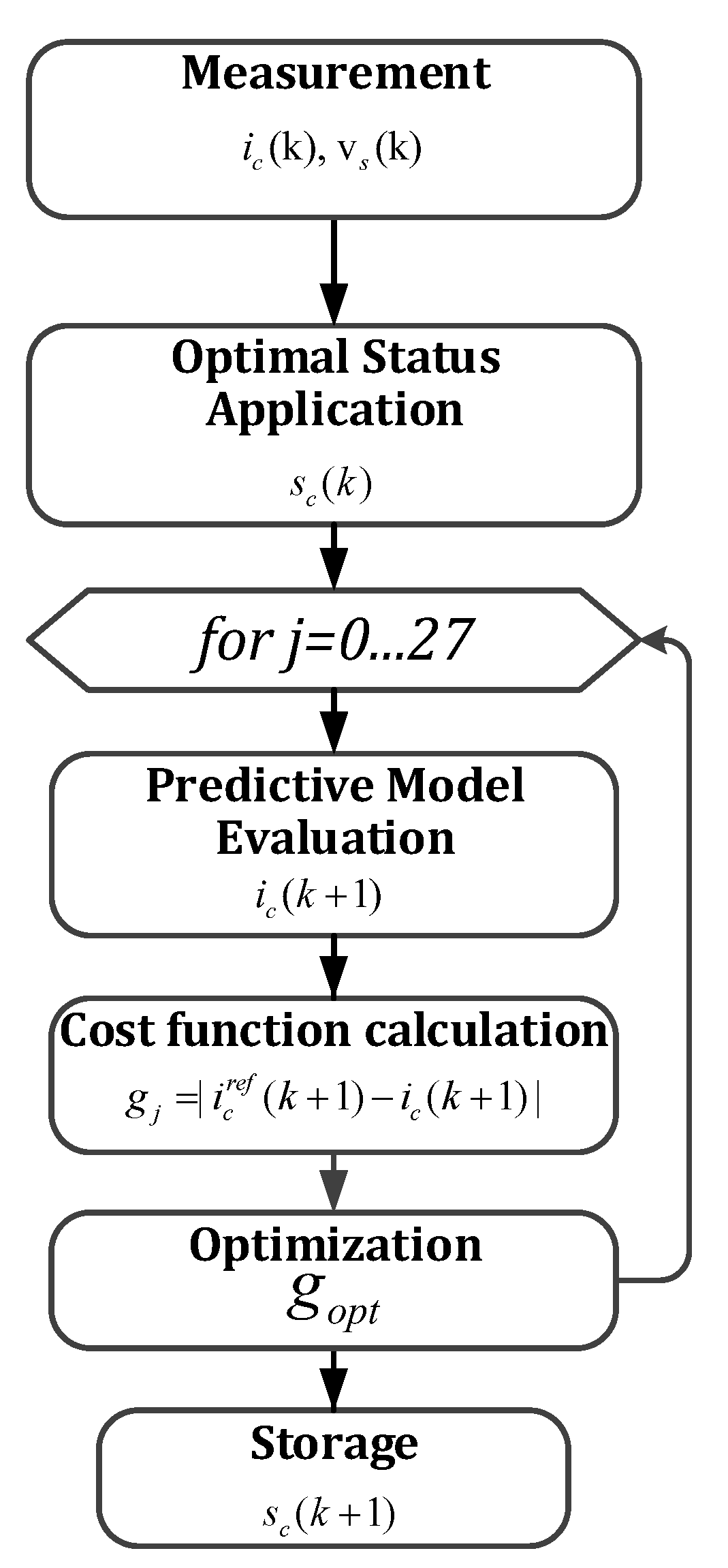
Figure 4.
Predictive control: Stability and robustness waveform.

Figure 5.
(a) Signal with undesired commutations. (b) Signal expected to be obtained.

Figure 6.
H-bridge zero states.

Figure 7.
Control scheme.

Figure 8.
Waveforms in transient state.

Figure 9.
Waveforms in steady state.
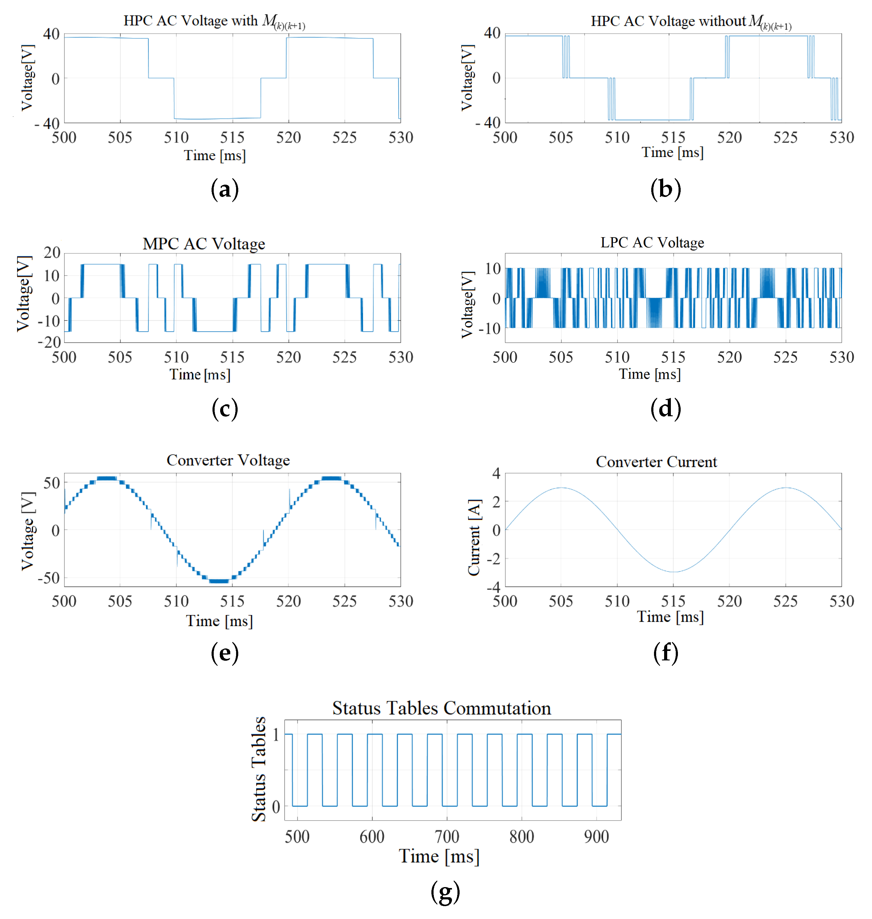
Figure 10.
Harmonic spectrum simulation. (a) Converter voltage, (b) converter current.

Figure 11.
HPC voltage, where the x-axis represents time with [5 ms/div] and y-axis represents voltage with [20 V/div]; (a) without restriction matrix, (b) with restriction matrix.
Figure 11.
HPC voltage, where the x-axis represents time with [5 ms/div] and y-axis represents voltage with [20 V/div]; (a) without restriction matrix, (b) with restriction matrix.

Figure 12.
Master control scheme.

Figure 13.
Prototype waveforms. (a) HPC DC voltage and converter current, (b) currents prior to the change in solar irradiance, and (c) currents after the change in solar irradiance.
Figure 13.
Prototype waveforms. (a) HPC DC voltage and converter current, (b) currents prior to the change in solar irradiance, and (c) currents after the change in solar irradiance.

Figure 14.
Experimental harmonic spectrum. (a) Converter voltage, (b) converter current.


Table 1.
Valid state matrix.
| State | HPC | MPC | LPC | Converter Voltage |
|---|---|---|---|---|
| 1 | − V9 − V3 − V1 | |||
| 2 | 0 | − V9 − V3 | ||
| 3 | 1 | − V9 − V3 + V1 | ||
| 4 | 0 | − V9 − V1 | ||
| 5 | 0 | 0 | − V9 | |
| 6 | 0 | 1 | − V9 + V1 | |
| 7 | 1 | − V9 + V3 − V1 | ||
| 8 | 1 | 0 | − V9 + V3 | |
| 9 | 1 | 1 | − V9 + V3 + V1 | |
| 10 | 0 | − V3 − V1 | ||
| 11 | 0 | 0 | − V3 | |
| 12 | 0 | 1 | − V3 + V1 | |
| 13 | 0 | 0 | − V1 | |
| 14 | 0 | 0 | 0 | 0 |
| 15 | 0 | 0 | 1 | V1 |
| 16 | 0 | 1 | + V3 − V1 | |
| 17 | 0 | 1 | 0 | + V3 |
| 18 | 0 | 1 | 1 | + V3 + V1 |
| 19 | 1 | + V9 − V3 − V1 | ||
| 20 | 1 | 0 | + V9 − V3 | |
| 21 | 1 | 1 | + V9 − V3 + V1 | |
| 22 | 1 | 0 | + V9 − V1 | |
| 23 | 1 | 0 | 0 | + V9 |
| 24 | 1 | 0 | 1 | + V9 + V1 |
| 25 | 1 | 1 | + V9 + V3 − V1 | |
| 26 | 1 | 1 | 0 | + V9 + V3 |
| 27 | 1 | 1 | 1 | + V9 + V3 + V1 |
Table 2.
Implementation parameters.
| Element | Description | Value |
|---|---|---|
| Converter resistance | 10 Ω | |
| Converter inductance | ||
| Grid voltage | ||
| Converter voltage | ||
| C | High-power cell (HPC) capacitor | |
| HPC direct current (DC) Reference | ||
| System frequency | ||
| Sampling time |
Table 3.
Constraint matrix.
| 1 | … | 9 | 10 | … | 18 | 19 | … | 27 | |
|---|---|---|---|---|---|---|---|---|---|
| 1 | 0 | … | 0 | 1 | … | 1 | 1 | … | 1 |
| ⋮ | ⋮ | ⋮ | ⋮ | ⋮ | ⋮ | ⋮ | |||
| 9 | 0 | … | 0 | 1 | … | 1 | 1 | … | 1 |
| 10 | 1 | … | 1 | 0 | … | 0 | 1 | … | 1 |
| ⋮ | ⋮ | ⋮ | ⋮ | ⋮ | ⋮ | ⋮ | |||
| 18 | 1 | … | 1 | 0 | … | 0 | 1 | … | 1 |
| 19 | 1 | … | 1 | 1 | … | 1 | 0 | … | 0 |
| ⋮ | ⋮ | ⋮ | ⋮ | ⋮ | ⋮ | ⋮ | |||
| 27 | 1 | … | 1 | 1 | … | 1 | 0 | … | 0 |
Table 4.
Total harmonic distortion (THD) comparison.
| THD | Simulation | Experimental |
|---|---|---|
Table 5.
Surveyed asymmetric multilevel topologies.
| Article | Topology | Modulation | Type | Application | Control | ||
|---|---|---|---|---|---|---|---|
| [38] | 7-level ACMLI | POD-PWM (4 kHz) | Sim | - | - | 1.12% | 14.83% |
| [38] | 7-level ACMLI | APOD-PWM (4 kHz) | Sim | - | - | 1.05% | 15.2% |
| [39] | 7-level asymmetric cascaded multilevel inverter | Hybrid carrier-based space vector modulation technique (HCBSVM) | Sim | PV | - | - | 3.71% |
| [41] | Cascaded 63-level asymmetrical multilevel inverter | Staircase | Sim | Ren. Energy | - | - | 3.85% |
| [40] | 5-level asymmetric cascaded multilevel inverter | Phase-shifted PWM | Sim | PV | - | - | 5.22% |
| [40] | 5-level asymmetric cascaded multilevel inverter | Level shifted PWM | Sim | PV | - | - | 3.84% |
| [43] | 15-level asymmetrical cascaded H-bridge multilevel inverter | PD-PWM (2 kHz) | Sim | PV | - | - | 6.03% |
| [44] | Asymmetric multilevel converter, composed of a two-level inverter and two floating cells per phase | Space vector | Sim | - | Predictive control | 0.55% | 4.9% |
| [45] | Asymmetric cascaded multilevel inverter with a single DC source | Space vector | Sim | - | Space vector control and predictive control | 1.5% | 12.9% |
| [46] | 15-level asymmetrical cascaded H-bridge multilevel inverter | - | Sim | PV | FS-MPC | <1% | - |
| [42] | 7-level asymmetric cascaded multilevel inverter | LS-PWM (1kHz) | Prot | PV | PI | 2.2% | 13.3% |
| [10] | 16:4:1 Asymmetric multilevel inverter | Space vectors with asymmetrical -staircase | Prot | - | - | - | <4% |
© 2020 by the authors. Licensee MDPI, Basel, Switzerland. This article is an open access article distributed under the terms and conditions of the Creative Commons Attribution (CC BY) license (http://creativecommons.org/licenses/by/4.0/).
Share and Cite
MDPI and ACS Style
Gaisse, P.; Muñoz, J.; Villalón, A.; Aliaga, R. Improved Predictive Control for an Asymmetric Multilevel Converter for Photovoltaic Energy. Sustainability 2020, 12, 6204. https://doi.org/10.3390/su12156204
AMA Style
Gaisse P, Muñoz J, Villalón A, Aliaga R. Improved Predictive Control for an Asymmetric Multilevel Converter for Photovoltaic Energy. Sustainability. 2020; 12(15):6204. https://doi.org/10.3390/su12156204
Chicago/Turabian StyleGaisse, Patricio, Javier Muñoz, Ariel Villalón, and Rodrigo Aliaga. 2020. "Improved Predictive Control for an Asymmetric Multilevel Converter for Photovoltaic Energy" Sustainability 12, no. 15: 6204. https://doi.org/10.3390/su12156204
Note that from the first issue of 2016, this journal uses article numbers instead of page numbers. See further details here.