A Forecasting and Prediction Methodology for Improving the Blue Economy Resilience to Climate Change in the Romanian Lower Danube Euroregion

Abstract

European Union (EU) policy encourages the development of a blue economy (BE) by unlocking the full economic potential of oceans, seas, lakes, rivers and other water resources, especially in member countries in which it represents a low contribution to the national economy (under 1%). However, climate change represents a main barrier to fully realizing a BE. Enabling conditions that will support the sustainable development of a BE and increase its climate resiliency must be promoted. Romania has high potential to contribute to the development of the EU BE due to its geographic characteristics, namely the presence of the Danube Delta-Black Sea macrosystem, which is part of the Romanian Lower Danube Euroregion (RLDE). Aquatic living resources represent a sector which can significantly contribute to the growth of the BE in the RLDE, a situation which imposes restrictions for both halting biodiversity loss and maintaining the proper conditions to maximize the benefits of the existing macrosystem. It is known that climate change causes water quality problems, accentuates water level fluctuations and loss of biodiversity and induces the destruction of habitats, which eventually leads to fish stock depletion. This paper aims to develop an analytical framework based on multiple linear predictive and forecast models that offers cost-efficient tools for the monitoring and control of water quality, fish stock dynamics and biodiversity in order to strengthen the resilience and adaptive capacity of the BE of the RLDE in the context of climate change. The following water-dependent variables were considered: total nitrogen (TN); total phosphorus (TP); dissolved oxygen (DO); pH; water temperature (wt); and water level, all of which were measured based on a series of 26 physicochemical indicators associated with 4 sampling areas within the RLDE (Brăila, Galați, Tulcea and Sulina counties). Predictive models based on fish species catches associated with the Galati County Danube River Basin segment and the “Danube Delta” Biosphere Reserve Administration territory were included in the analytical framework to establish an efficient tool for monitoring fish stock dynamics and structures as well as identify methods of controlling fish biodiversity in the RLDE to enhance the sustainable development and resilience of the already-existing BE and its expansion (blue growth) in the context of aquatic environment climate variation. The study area reflects the integrated approach of the emerging BE, focused on the ocean, seas, lakes and rivers according to the United Nations Agenda. The results emphasized the vulnerability of the RLDE to climate change, a situation revealed by the water level, air temperature and water quality parameter trend lines and forecast models. Considering the sampling design applied within the RLDE, it can be stated that the Tulcea county Danube sector was less affected by climate change compared with the Galați county sector as confirmed by water TN and TP forecast analysis, which revealed higher increasing trends in Galați compared with Tulcea. The fish stock biodiversity was proven to be affected by global warming within the RLDE, since peaceful species had a higher upward trend compared with predatory species. Water level and air temperature forecasting analysis proved to be an important tool for climate change monitoring in the study area. The resulting analytical framework confirmed that time series methods could be used together with machine learning prediction methods to highlight their synergetic abilities for monitoring and predicting the impact of climate change on the marine living resources of the BE sector within the RLDE. The forecasting models developed in the present study were meant to be used as methods of revealing future information, making it possible for decision makers to adopt proper management solutions to prevent or limit the negative impacts of climate change on the BE. Through the identified independent variables, prediction models offer a solution for managing the dependent variables and the possibility of performing less cost-demanding aquatic environment monitoring activities.

1. Introduction

1.1. EU Blue Economy and Blue Growth

In the scientific literature, a blue economy (BE) is most widely associated with actions related to the governance and management of seas and oceans [1,2]. There is no widely accepted definition of the term BE [2]. Therefore, according to some authors [3], the definition of a BE includes aquatic and marine spaces (e.g., seas, coasts, lakes, wetlands, floodplains, rivers and underground water resources) while also covering a variety of production sectors including fishing, aquaculture, tourism, shipbuilding, underwater mining, transport, bioprospecting and other related activities. Other research papers [4] pointed out that a BE encompasses all economic activities related to the oceans, seas and coasts, covering a wide range of interlinked established and emerging sectors. The BE is considered a consequence of the growing worldwide interest in the growth of water-based activities [5] seeking to curb biodiversity loss while stimulating economic development [6]. The EU concept of a BE includes all economic activities related to the oceans, seas and coasts, which includes a wide range of interlinked sectors [7] compared with the World Bank BE concept, which is strictly based on the sustainable use of ocean resources [8]. According to the European Commission Report on BEs elaborated in 2021 [9], the EU BE includes a series of established sectors such as marine living resources, marine extraction of non-living resources, maritime transport, port activities, shipbuilding and repair as well as coastal tourism, all of which are considered highly important for the development of the EU economy in addition to emerging sectors such as marine renewable energy, BE biotechnology, desalination, marine minerals, marine defense, security and surveillance. The importance of the EU BE is revealed by the fact that it directly employs over 4 million people (1.8% of the overall EU economy), with over EUR 600 billion in turnover and almost EUR 200 billion in gross value added (1.3% of the overall EU economy) [7]. Marine living resources represent the second most important sector for the EU BE which, according to Eurostat, employs on average 573,000 persons per year (more than 15% of the total EU BE employment) and yields an annual average gross value added (GVA) of over EUR 18 billion, which has been expanding since 2013. This sector is mostly composed of fisheries and aquaculture, as well as aquatic animal processing and distribution activities. Since both processing and distribution activities dependent on the fish supply and marine living resources represent a key sector of the EU BE, the fisheries and aquaculture subsectors can be ranked as the most important for ensuring blue growth (BG). Recent research [10] has characterized BG as an emerging concept which aims to achieve economic growth based on the exploitation of marine resources while avoiding their degradation, excessive use and pollution. The presence of BG is characterized by the key aspects demanded by a BE to overcome economic, social and environmental challenges [11]. Martínez-Vázquez et al. (2021) revealed that the relationship between a BE and a circular economy (CE) is mediated by BG and emphasizes the link between fisheries as a BE component and water as a CE component [11]. This is valid since fisheries depend on water, as their life cycle depends on this natural environment and both its conditions (e.g., quality, temperature and salinity) [12] and its proper management influences the sustainability and conservation of marine species [8]. Fisheries and water are important components linked by EU BG, a situation also confirmed by the EU Common Fisheries Policy (CFP), which promotes fish consumption and trade, underlining the value of fish to society from both the social and ecological perspectives [13]. Thus, it is important to maintain the aquatic systems in good health by constant monitoring and control of the water quality, water level and fish stock status to improve BE resilience to emerging challenges.

1.2. Impact of Climate Change on Aquatic Ecosystems

Climate change can be considered one of the main challenges which a BE has to deal with, since it affects both fisheries and aquaculture and, therefore, the marine living resources subsector. Climate variation influences water quality, food security and the socio-economies of different regions [14]. It also has a significant effect on stock abundance dynamics [15] and generally on biological assets [16]. Thus, fish stock assessment highly depends on the ability to predict the impacts of climate change on the dynamics of aquatic ecosystems [15,17]. Climate change impacts aquatic ecosystems by altering biodiversity patterns [18,19], the abundance and distribution of species (15), biological interactions, phenology and organism physiology [20,21]. Several research studies [22,23] revealed that the impacts of climate change upon aquatic biodiversity are expected to intensify soon. Changes in distributions and the community structures of fish species may influence fishing activities and have socioeconomic impacts on vulnerable coastal communities [24,25]. An increase in water temperature and water level are both primary indicators of climate change [26,27,28]. According to several studies [29,30,31], water level fluctuations could have a major impact on communities of fish species within rivers and, therefore, on commercial fish stocks, in addition to a considerable influence upon the topography of the basin in time and space [32]. Under climate change, the supply of water resources is unlikely to remain constant, and regional water availability is no longer assured [33].

Therefore, water level variations directly influence the abundance of periphyton, aquatic macrophytes and benthos and can indirectly affect phytoplankton and zooplankton [34], which are important nutritional sources for fish stocks. Moreover, according to previous studies [35], fish stocks can be affected if the water level changes rapidly during the reproduction period, a situation that applies particularly to substrate spawning fish species. Additionally, the nitrogen and phosphorus concentrations in water will increase due to global warming [36,37]. Therefore, a rise in temperature increases the concentration of soluble phosphate in the water [36] and salter nitrogen cycling processes affecting terrestrial and aquatic ecosystems, as well as human health [37].

According to several studies [38,39], climate change may alter the discharge regime of rivers and, therefore, their magnitude, duration, frequency, rate and timing of discharge events. Dysfunctionalities related to water level dynamics can reduce estuary flushing rates if river flow decreases, while if the flow rate increases, the N and P upward loading of aquatic ecosystems will appear by transferring these nutrients from agriculture fields, as confirmed by other studies. Nutrients, especially phosphorus and nitrogen from various sources, and increasing temperatures constitute the major causes of degradation of the aquatic ecosystems, namely in the form of eutrophication [40]. Climate change will significantly alter nitrogen cycling processes, with a negative impact on aquatic ecosystems as well as human health [37]. Furthermore, according to recent studies [41,42,43], the oxygen content of aquatic environments has declined substantially in the past few decades as a direct consequence of global warming. Therefore, surface water oxygen solubility decreases with increasing temperatures [41]. The water pH is also affected by global warming and, more specifically, by the increase of atmospheric CO₂. This increases ocean acidification [44]. Water is considered a scarce resource in the modern era (given the rapid growth of populations and enormous water-intensive industries); thus, competition for water rights among sectors usually results in conflicts of interest [45]. This can generate serious shortages within a BE [46] and give rise to already-existing climate change pressure. Thus, according to the authors of [47], water use equilibrium is dependent on climate-induced impact.

1.3. Romania BE in Relation to Climate Change

Although the EU targets the development of a BE, there are still member countries that register low contributions of BEs to their national economies (under 1%), such as Romania, Slovenia and Belgium. Despite these results, Romania has significant potential for sustaining the European Union BG strategy, especially due to its geographical characteristics [48]. This potential is based on the presence of the Danube River (1075 km out of a total of 2857 km are in Romanian territory) connected to the Black Sea and its marginal ecosystems, with the vast surface of the Danube Delta (3446 km² of a total of 4152 km² is in Romania territory) and many natural lakes, canals and ponds present within the Romanian Lower Danube Euroregion (Brăila, Galați and Tulcea county). According to Eurostat data, the Romanian marine living resources sector implies that there is an average of 7000 employed persons and an annual GVA of approximately EUR 64 million. The Romanian Lower Danube Euroregion (RLDE) represents the most significant contribution to the marine living resources sector. This is due to both high fishery and aquaculture activities. The country’s national BE is mostly based on the Danube–Danube Delta–Black Sea macrosystem. This presupposes strict aquatic environment monitoring and control activity, which are essential for the proper functionality of a BE. This activity can be performed by using prediction and forecasting methodologies facilitating the control and identifying in advance the effects of possible threats, such as climate change, on the water’s physicochemical parameters and the fish stocks status. According to different scenarios, the projected extinction rates of aquatic biodiversity are higher compared with those of terrestrial biodiversity [49] due to climate change, which is increasingly threatening fish, resulting in an uncertain future for both wild fish diversity and global fisheries [50,51]. What is more, climate warming-induced environmental changes can negatively affect several migratory fish species which are characterized by a high degree of synchronization between their reproductive cycles and seasonal river flow dynamics [24]. Most fish species respond to climate change through biological adaptation [52], aquatic area shifting [53] and even extinction [54]. Fish growth alteration is considered a main direct and common consequence of climate change [55] and can have long-term influences on stock dynamics and characteristics [56]. Predicting the impacts of climate change on aquatic ecosystems based on fish stocks response can represent a monitoring solution for improving the resilience management plan, a fact confirmed by other studies [57,58]. However, climate change affects aquatic environments from different climate zones in various manners [59], and its effect is specifically attributed to each fish species. Therefore, the impact prediction models must be unique for each aquatic ecosystem. Studies [60,61] which analyzed the climate change effect on the Danube–Danube Delta–Black Sea macrosystem reported an upward trend for eutrophication within the Danube River Basin, with urban settlement and agriculture contributing majorly to amplifying the nitrogen and phosphorus emissions, respectively [61]. The monitoring of aquatic macrosystem water quality is essential for developing a BE and indicates trends over time, which offers the possibility of identifying the sustainability of a BE and selecting the most appropriate direct remedial actions. Additionally, an evaluation of water quality parameters is necessary to plan and develop better water resource management [62,63].

Several papers approached the subject of water quality in the Danube River. For instance, Mănoiu and Crăciun (2021) realized a thorough review of the water quality trends in the Danube River [64], focusing on Serbia, Romania, Slovakia, Hungary, Germany and Austria. They observed reductions in the nutrient loads in the water of the Danube River; however, the river is still at risk of degradation due to organic pollution. Other studies calculated the Water Quality Index (WQI), which integrates different physicochemical parameters into the formula and synthetizes the data into a single number to highlight the ecological status of the water body in Chiciu, Romania [65] near Galați, Romania [66], between the sector of Brăila and Tulcea within Romania [67]. All authors highlighted in their studies a general good water quality status in the Danube River. Frîncu (2021) developed a complex methodology for assessing the water quality of the Lower Danube [68] using the WQI and Principal Component Analysis (PCA) between the years 1996 of 2017. In their study, Krtolica et al. (2021) predicted the Danube water quality by using macrophyte binary data through neural network modeling [69]. However, none of the mentioned studies approached the interlinked impact involving the water quality and fish stocks status within the Danube-Danube Delta-Black Sea macrosystem.

1.4. Deep Learning Approach in Aquatic Ecosystems

Traditional methods for synthetically evaluating the water quality of aquatic ecosystems have been replaced by new modeling approaches, multivariate statistical techniques, artificial neural networks, artificial intelligence, ARIMA, SARIMA or ETS models. For example, artificial neural network models were used to predict the dissolved oxygen and biochemical oxygen demand by other nutrients or basic physicochemical parameters such as explanatory variables [70,71], while others aimed to explore the relationship between nutrients and biological quality elements [72].

The water quality variables are changing continuously through time. This dynamic process containing random error components with stochastic variations in space and time is difficult to model or explain with normal analytical procedures. Still, the analysis of time series datasets containing water quality parameters using ARIMA-type models provided relevant results [73]. Long-term trends in water quality can reveal information about chemical, biological and physical changes and variations due to manmade and seasonal interventions. For example, in [74], the authors developed an ARIMA model to forecast several water quality variables like the pH, color (TCU), turbidity (ppm), Al³⁺ (ppm), Fe²⁺ (ppm), NH⁴⁺ (ppm) and Mn²⁺ (ppm) through the respective hydrological variables, namely rainfall and river discharge, for the Johor River in Malaysia. In [75], it is also emphasized that weather parameters such as humidity, wind speed, rainfall or air temperature are non-linear and complex phenomena involving mathematical simulation and proper modeling for correct forecasting. Aside from ARIMA, the authors also used Exponential Smoothing (ETS) models to forecast the exemplified parameters. The seasonal variation (seasonal autoregressive integrated moving average (SARIMA)) model was also used in different water-related studies. For example, in [76], the authors used a SARIMA model to forecast the water level of the Sungai Bedup River in Malaysia. Aside from water quality forecasting, the analysis of the relationship between some physicochemical parameters is also of great interest, as it could help to determine the concentrations of certain water parameters with the use of minimal equipment. This is important because developing countries lack the standard water analysis equipment—specifically, the adequately trained personnel—and many researchers are discouraged from executing water quality research [77]. A study of the specific scientific literature revealed a series of empirical research which had been performed to investigate the relationship between economic growth and environment quality [78,79]. Thus, in [77], by using multiple linear regression, the authors identified the mathematical relationship among several physicochemical parameters (e.g., turbidity, electrical conductivity (EC), pH, alkalinity, chloride ion (Cl⁻), dissolved oxygen (DO) and total hardness) that could help to perform future determinations with the use of minimal equipment. Therefore, prediction models such as MLR can represent a suitable cost-effective method which can partially substitute the standard, routine laboratory analysis, offering accessible monitoring of aquatic environments. Another example can be found in [80], where monthly water quality datasets from 10 stations on the Tigris River within Baghdad for the year 2016 were studied. The Water Quality Index (WQI) and a Water Quality Model (WQM) were calculated by using 11 important parameters (Al³⁺, F¹⁻, NO₂¹⁻, NO₃¹⁻, NH₃, temperature, total alkalinity, turbidity, total hardness, Ca²⁺, Cl¹⁻, Mg²⁺, pH, electrical conductivity, SO₄²⁻, TDS, Fe²⁺, SiO₂, PO₄³⁻, DO, BOD5, COD and Na¹⁺) and multiple linear regression analysis.

In [81], the authors elaborated on the widely applicable water economics models which incorporate economic and environmental components, identifying the response of the agricultural production sector to climate change as part of the BE. Other studies [82] developed water models widely applicable in the BE by considering all major water use sectors.

1.5. Aim and Uniqueness of This Study

The current study aims to use the autoregressive integrated moving average (ARIMA), seasonal autoregressive integrated moving average (SARIMA), error, trend and seasonality (ETS) and multiple linear regression (MLR) models to develop an analytical framework which aims to strengthen the resilience and adaptive capacity of a BE within the context of climate change in the Romanian Lower Danube Euroregion (RLDE). If the ARIMA, SARIMA and ETS methods are used for time series forecasting, the multiple linear regression technique should be the preferred choice if the relation between the predictors and the dependent variable displays a linear pattern. Therefore, this study led to the development of several predictive forecasting models that are suitably used for determining the following water-dependent variables: total nitrogen (TN), total phosphorus (TN), dissolved oxygen (DO), pH, water temperature (wt) and water level, based on a series of 26 indicators (independent variables). Additionally, the research targets to elaborate several fish species structure predictive models that can be used to assure a better aquatic environment resilience framework related to climate variation, guaranteeing BG within the RLDE.

The study’s uniqueness is underlined first; no other similar research was conducted within the RLDE. Additionally, we offer a holistic approach to the Danube–Danube Delta–Black Sea macrosystem, since we consider the water quality parameters, water level variation and fish species interactions. The targeted framework of this research is meant to be used for monitoring the water quality, water level and fish stock status but also for identifying methods of controlling the ecological balance of fish species. The specificity of the research area was considered while designing the experimental data collection, revealing an original approach in the aquatic macrosystem-developed methodology for monitoring, evaluation and control.

2. Materials and Methods

2.1. Study Area

The present paper studies water level, water quality and fish catch data from the RLDE. The Brăila, Galați, Tulcea and Sulina hydrometric stations (Figure 1) were considered for characterizing the RLDE in terms of water level, water temperature and air temperature, since these are considered key monitoring points due to high anthropogenic pressure from heavy industry, agriculture, aquaculture and navigation activities. Additionally, the highest air temperatures in Romania are attributed to this region, with a record of an absolute maximum air temperature of 44.5 °C recorded in Brăila county. The desertification process within this region is the most intense [83] in Romania and could lead to unfavorable conditions for assuring BG.

The Danube water quality data was collected from the Galați and Tulcea sampling points, since Galați and Tulcea have the most intense naval industry and port activity, therefore being exposed to water pollution.

Data relating to fish catches were recorded from the Galati county Danube River Basin segment (L1) and from the “Danube Delta” Biosphere Reserve Administration territory (L2) (Figure 1). The data on fish catches are monitored within these two sectors because of administrative division of the RLDE territory.

2.2. Dataset Description

The present research is based on a dataset which is divided in two groups, specifically 26 physicochemical parameters (

Table 1. Dataset of physicochemical parameters.

Parameter	Measurement Unit	Standard Method of Determination	Sampling Area
Water level (wt)	(cm)	SOP 2043	Brăila, Galați, Tulcea, Sulina
Water temperature (wt)	(°C)	Sensor’s methods	Galați, Tulcea
Air temperature (aw)	(°C)	Sensor’s method	Galați, Tulcea
Total suspended solids (TSS)	(mg/L)	SE EN 875:2005	Galați, Tulcea
Turbidity (tb)	(NTU)	SR EN ISO 7027:2001	Galați
Dissolved oxygen (DO)	(mg/L)	SR EN ISO 5814:2013	Galați, Tulcea
Dissolved oxygen saturation (DO sat.)	(%)	-	Galați, Tulcea
Biochemical oxygen demand (BOD5)	(mg/L)	SR EN 1899:2:2002	Galați, Tulcea
Chemical oxygen demand (COD)	(mg/L)	SR EN 1484:2001	Galați
Total organic carbon (TOC)	(mg/L)	SR EN 1484:2001	Galați
Electrical conductivity (EC)	(µS/cm)	SE EN 27888:1997	Galați, Tulcea
Fixed solids (FS)	(mg/L)	STAS 9187:1984	Galați, Tulcea
Calcium (Ca)	(mg/L)	SE ISO 6058:2008	Galați, Tulcea
Magnesium (Mg)	(mg/L)	SE ISO 6059:2008	Galați, Tulcea
Total hardness (TH)	(°G)	SR ISO 6059:2008	Galați
Chloride (Cl)	(mg/L)	SE ISO 9297:2001	Galați, Tulcea
Sulfate (SO4)	(mg/L)	EPA 9038:1986	Galați, Tulcea
pH	(upH)	SR ISO 10523:2012	Galați, Tulcea
Alkalinity (Alk)	(mmol/L)	SR ISO 9963-1/A99:2002	Galați, Tulcea
Bicarbonates (Bi)	(mg/L)	SR ISO 9963-1/A99:2002	Galați, Tulcea
Ammonium-nitrogen (N-NH4)	(mg/L)	SR ISO 7150-1:2001	Galați, Tulcea
Nitrite-nitrogen (N-NO2)	(mg/L)	SR ISO 26777/C91:2006	Galați, Tulcea
Nitrate-nitrogen (N-NO3)	(mg/L)	SR ISO 7890-3:2000	Galați, Tulcea
Total nitrogen (TN)	(mg/L)	SR EN 12260:2004	Galați, Tulcea
Orthophosphate as phosphorus (P-PO4)	(mg/L)	SR EN ISO6878:2005	Galați, Tulcea
Total phosphorus (TP)	(mg/L)	SR EN ISO 6878:2005	Galați, Tulcea

) and 27 fish catch parameters (

Table 2. Dataset of fish catches.

Fish Species	Abbreviation	Study Area
Abramis brama danubii (freshwater bream)	Fbr	L1, L2
Alburnus alburnus (common bleak)	Cbl	L1
Alosa caspia (Caspian shad)	Csh	L2
Alosa immaculata (Pontic shad)	Psh	L1, L2
Aspius aspius (asp)	Asp	L1, L2
Barbus barbus (common barbel)	Cbb	L1, L2
Blicca bjoerkna (white bream)	Wbr	L1, L2
Carassius gibelio (Prusian carp)	Pcp	L1, L2
Other cyprinids	Ocp	L1, L2
Cyprinus carpio carpio (common carp)	Ccp	L1, L2
Esox lucius (pike)	Pk	L1, L2
Liza aurata (golden grey mullet)	Ggm	L2
Mullus barbatus ponticus (red mullet)	Rmt	L2
Neogobius kessleri (bighead goby)	Bgb	L2
Pelecus cultratus (sabre carp)	Scp	L2
Perca fluviatilis fluviatilis (perch)	Prc	L2
Psetta maxima maeotica (turbot)	Tbt	L2
Raja clavata (thornback ray)	Tr	L2
Rutilus rutilus carpathorosicus (roach)	Rch	L1, L2
Sander lucioperca (pikeperch)	PkPrc	L1, L2
Scardinius erytrophthalmus (common rudd)	Crd	L1, L2
Silurus glanis(catfish)	Ctf	L1, L2
Sprattus sprattus (European sprat)	Esp	L2
Tinca tinca (tench)	Tnch	L2
Trachurus ponticus (horse mackerel)	Hmk	L2
Vimba vimba carinata (vimba)	Vmb	L1, L2

). The first group (Table 1) consisted of 7668 samples, of which 2340 belonged to Tulcea county, 2448 belonged to Galați county and 1440 belonged to both Brăila and Sulina. Data surrounding the Danube River water level, water temperature and air temperature parameters, presented in Table 1, were collected daily between 2017 and 2020. Furthermore, the rest of the data related to Danube water quality (presented in Table 1) was collected monthly from Galați county between 2017 and 2020 and once every 2 months from Tulcea county between 2015 and 2020. The dataset’s standard method of determination is presented for each of the first group’s parameters in Table 1.

The second group (Table 2) consisted of 340 samples, of which 90 were for L1 and 250 were for L2. All reported catches associated with the main RLDE fish species were considered.

2.3. The Analytical Framework Forecasting and Prediction Methodology

2.3.1. Multiple Linear Regression (MLR) Method

The linear approach used in this research was performed by identifying and testing multiple linear regression models (Equation (1)) by using the stepwise selection methods (with the inclusion criteria set at p < 0.05) for choosing the most relevant predictors:

$$Y={\alpha }_1\times X_1+{\alpha }_2\times X_2+\dots +{\alpha }_p\times X_p+\beta +e$$

(1)

where X₁, X₂ … X_p are the predictor variables; β is the intercept; α₁, α₂ … α_p are the independent variable coefficients describing the contribution of each predictor in determining the dependent variable; e is the residual term indicating the difference between the actual and the fitted response value; and Y is the dependent variable.

The overfitting situation was avoided by using dimensionality reduction and cross-validation. When the number of features was high, choosing the optimal features could improve the model reliability; therefore, all MLR models considered the stepwise regression method to reduce the model complexity, leading to an easier interpretation. For the validation of the MLR models, we used the adjusted R-sq statistical indicator that penalized the model when there were many parameters that were not contributing to explaining the variance of the dependent variable.

The multiple linear regressions presented in the current research also took into consideration the Variance Inflation Factor (VIF), which measured the effect of multicollinearity among the predictors. The VIF measures how much the variance of an estimated regression coefficient increases if the predictors are correlated. The reference VIF value was 10, but the developed models presented VIF values far less than 10.

The multiple linear models were validated using previously unseen data, comparing the real values with the predicted ones. The overall dataset was split in two: a training dataset and a test dataset. The training dataset contained 80% of the data, while the remaining 20% of the data contained previously unseen samples.

2.3.2. Time Series Analysis

For validating the future trends of the interest parameters, the current research implemented three types of time series analysis: (1) error, trend and seasonality (ETS) exponential smoothing, (2) ARIMA and (3) SARIMA.

The exponential smoothing method, described in [84] and [85], represents a successful forecasting method based on weighted averages of past observations, with the weights being exponentially reduced as the observations get older (Equation (2)):

$${\widehat{y}}_{T+h|T}=y_T , h=1,2,\dots ,n$$

(2)

According to this method, the most recent observation is the important one. Thus, all future forecasts should be equal to an average of the observed data (Equation (3)):

$${\widehat{y}}_{T+h|T}=\frac{1}{T}{\displaystyle \sum }_{t=1}^T{y}_t h=1,2\dots ,n$$

(3)

This time series model can be transformed by considering larger weights for more recent observations, with the forecasts being calculated by using weighted averages and the weights decreasing exponentially as the observations come from further in the past (Equation (4)):

$${\widehat{y}}_{T+h|T}=\alpha y_T+\alpha \left(1-\alpha \right)y_{T-1}+\alpha (1-{\alpha }^2)y_{T-2}+\dots$$

(4)

where 0 ≤ α ≤ 1 is the smoothing parameter. As an example, the forecast for time T + 1 represents a weighted average of the observations in the series y1…yT, with the parameter α controlling the rate at which the weights decrease.

The Holt [86] exponential time series model allows the forecasting of data presenting a trend by using both a forecast equation and smoothing equations (Equations (5)–(7)):

$$Forecast equation: {\widehat{y}}_{t+h|t}=l_t+h{b}_t$$

(5)

$$Trend equation: b_t={\beta }^{*}\left(l_t-l_{t-1}\right)+\left(1-{\beta }^{*}\right)b_{t-1}$$

(6)

$$evel equation: l_t=\alpha y_t+\left(1-\alpha \right)\left(l_{t-1}+b_{t-1}\right)$$

(7)

where ℓt is the estimate of the level of the series at time t, bt is the estimate of the trend (slope) of the series at time t, α is the smoothing parameter for the level, 0 ≤ α ≤ 1, β* is the smoothing parameter for the trend, and 0 ≤ β* ≤ 1.

The ARIMA forecasting model is constructed as follows, with y denoting the dth difference of Y (Equations (8)–(11)):

$$d=0 \to y_t=Y_t$$

(8)

$$d=1 \to y_t=Y_t-Y_{t-1}$$

(9)

$$d=2 \to y_t=(Y_t-Y_{t-1})-(Y_{t-1}-Y_{t-2})$$

(10)

$$d=2 \to y_t=(Y_t-Y_{t-1})-(Y_{t-1}-Y_{t-2})$$

(11)

The moving average parameters (θs) were considered with a negative sign in the equation, according to the convention introduced by Box and Jenkins. To determine the optimal values for the p, d and q hyperparameters, the order of differencing (d value, the minimum differencing required to get a near-stationary series) was determined by using the autocorrelation function (ACF). For testing the stationarity of the time series, the augmented Dickey–Fuller test was used. For determining the p value (if the model needed any AR terms), the partial autocorrelation (PACF) plot was used. Lastly, the q value—the order of the MA term—was also determined by using an ACF plot, in which the number of lags above the significance line determined the q value. An extension of the ARIMA model that was used in the current research is SARIMA, a model that is used when there is the phenomenon of seasonality at the level of the variable for which the forecast is desired. The acronym SARIMA comes from Seasonal Autoregressive Integrated Moving Average and is a method of predicting univariate time series that contain trends and seasonality. The seasonal part of the model refers to terms that are very similar to the non-seasonal components of the model but involve changes in the seasonal period. SARIMA models consist of two parts: a trend component containing three elements (autoregressive trend, trend integration and moving order trend) and a seasonal component containing four elements (autoregressive seasonality, seasonal difference order, moving average order of seasonality and the number of steps of a single seasonal period). A seasonal ARIMA model uses differentiation at a lag equal to the number of periods to eliminate seasonal effects, just as gap differentiation eliminates the trend and that of forecast delays introduces a moving term [87]. Thus, a seasonal ARIMA model will be written in the following form (Equation (12)):

$$SARIMA\left(p,d,q\right){\left(P,D,Q\right)}_m$$

(12)

where p represents the autoregressive order of the trend, d represents the integration order at which the trend was stationary, q is the moving average order of the trend, P is the autoregressive order of seasonality, D is the order of integrating seasonality, Q is the order of the moving average of the seasonality, and m is the number of periods in which the seasonality is observed.

For example, an ARIMA model (1,1,1) (1,1,1) _m can be written as follows (Equation (13)):

$$\left(1-{\varphi }_{1}B\right)\left(1-{\mathsf{\Phi }}_1{B}^m\right)\left(1-B\right)\left(1-B^m\right)y_t=\left(1+{\theta }_{1}B\right)\left(1+{\mathsf{\Theta }}_1{B}^m\right){\epsilon }_t$$

(13)

3. Results and Discussion

3.1. Water Level Forecast Analysis

The water level is an important indicator of the impact of climate change on water ecosystems. According to other studies [88], an average increase in temperature by 0.74 °C has been recorded in the previous 100 years. The fluctuation of sea water temperature may affect water quality parameters and therefore the biodiversity of aquatic ecosystems. Water level fluctuations affect not only the marine living resources sector but also other sectors of a BE, such as maritime transport, port activities and coastal tourism. Therefore, an analytical framework based on water level time series analysis proves to be useful to improving BG’s resilience to climate change. The RLDE peculiarity is represented by the presence of the Danube River–Danube Delta–Black Sea macrosystem. Thus, data from four sampling points, placed in different sectors of this macrosystem, were collected, as presented in Figure 1. The analysis of forecast models requires the time series to be stationary. Therefore, the augmented Dickey–Fuller (ADF) test was applied. To achieve this, two scenarios will be formulated: the first scenario considers the series as stationary, and the second scenario considers the series as non-stationary. The results of the ADF test indicate the following values: −2.859 for Brăila, −3.622 for Galați, −3.14 for Tulcea and −3.630 for Sulina. All values were under the ADF critical value (−2.863), and therefore, all four data series were stationary. For the time series afferent to the Brăila, Galați and Tulcea sampling points, a second-order autoregressive type model (AR 2) was considered, since the correlograms emphasized that at time t = 2, the partial autocorrelation coefficient (PAC) manifested a sudden decrease. The statistical analysis of the proposed autoregressive models revealed that homoscedasticity was not fulfilled in any of the models, a fact which concludes that the errors did not have a constant dispersion. If this situation was ignored, the estimators of the model parameters would not be efficient and would not have a maximum likelihood. To eliminate this phenomenon, the models were transformed into Autoregressive Conditional Heteroscedasticity (ARCH) models that aimed to include the repetitive manifestations of the occurrence of forecast errors in several time sequences. Therefore, at the Brăila sampling point, the following forecast model for the Danube River water level was elaborated (Equation (14)). The model emphasized that if the water level increased by 1 m the day before, the current level was bound to increase by 1.857 m. Moreover, if it is 2 days before the water level increases by 1 m, then the current level will decrease by 0.861 m. All estimator parameters are significant, and the model is plausible (R-squared coefficient of determination is 99.90%) and can be used in the forecast:

$$\begin{array}{c}waterleve{l}_t=0.716+1.857\times waterleve{l}_{t-1}-0.861\times waterleve{l}_{t-2}\end{array}$$

(14)

The forecast model elaborated based on the water level dataset for the Danube River sampling point in Galați (Equation (15)) revealed that if the water level increased 1 m the day before, the current level would increase by 1.820 m. Additionally, if the water level increased by 1 m 2 days before, then the current level would decrease by 0.823 m. All estimator parameters were significant, and the model was plausible (R-squared coefficient of determination was 99.90%) and could be used in the forecast. Both models (Equations (14) and (15)) were similar, which could be explained by the low geographical distance between the sampling points of both Brăila and Galați:

$$\begin{array}{c}waterleve{l}_t=0.769+1.820\times waterleve{l}_{t-1}-0.823\times waterleve{l}_{t-2}\end{array}$$

(15)

The forecast model for the water level of the Danube River at the Tulcea sampling point (Equation (16)) revealed that water level depended on the moments of both one and two antecedent days such that a 1-m increase in the water level the day before would generate a present-day level increase of 1.735 m. At the same time, if the water level increased by 1 m 2 days before, then the current level would decrease by 0.738 m. All estimator parameters were significant, and the model is plausible and can be used in the forecast:

$$\begin{array}{c}waterleve{l}_t=0.384+1.735\times waterleve{l}_{t-1}-0.738\times waterleve{l}_{t-2}\end{array}$$

(16)

To generate the Danube River water level forecast model for the Sulina sampling point, the data series must be stabilized, since it has an oscillating evolution. Therefore, the data series was placed into a logarithm previously. The model also started with a third-order autoregressive model. Considering that the errors were heteroscedastic, the model was transformed into an ARCH type. The Sulina forecast model (Equation (17)) revealed that the current water level of the Danube River depended on moments 1 day, 2 days and 3 days prior such that if a 1-m increase was registered the day before, the current level would decrease by 0.100 m. At the same time, if the water level would increase by 1 m 2 days before, then the current level would decrease by 0.188 m. An increase by 1 m 3 days before would lead to a decrease by 0.116 m for the current level. All estimator parameters were significant, although the model was not plausible:

$$\begin{array}{c}dlwaterleve{l}_t=-0.100\times dlwaterleve{l}_{t-1}-0.188\times dlwaterleve{l}_{t-2}-0.116\times dlwaterleve{l}_{t-3 }\end{array}$$

(17)

All four time series models (Equations (14)–(17)) can be used to forecast the water level of the Danube River in Brăila, Galați, Tulcea and Sulina. This can be useful in elaborating RLDE BG management plans, thereby targeting the optimization of all BE activities and assuring a positive synergy between all blue sectors.

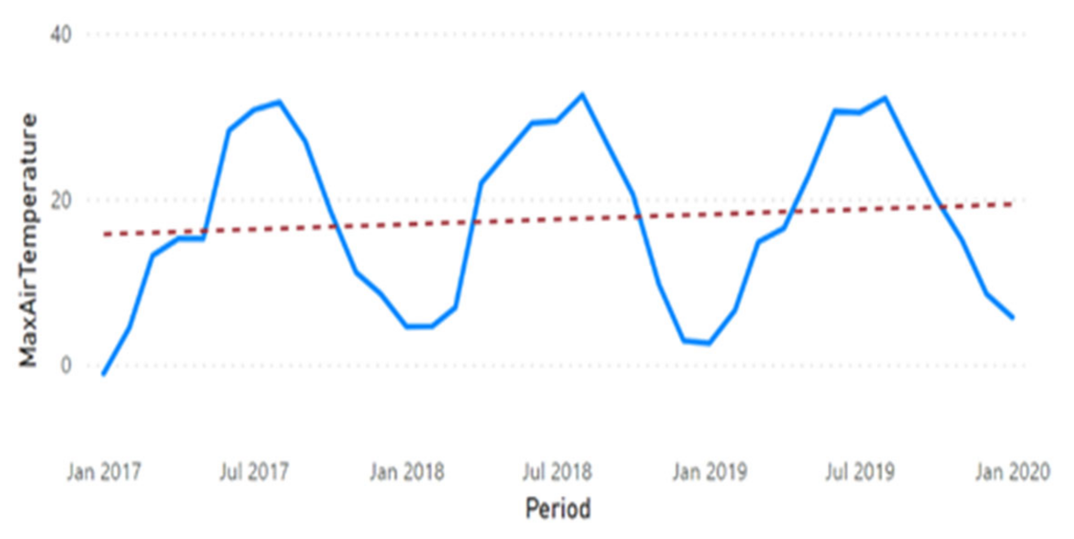
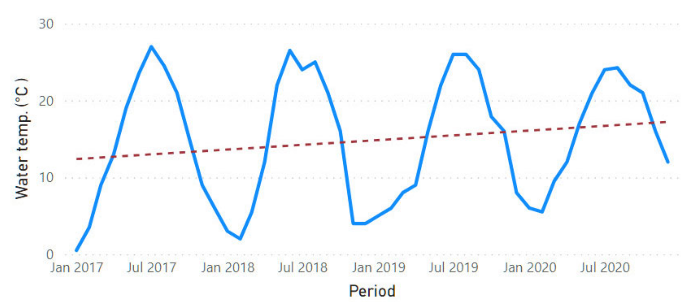
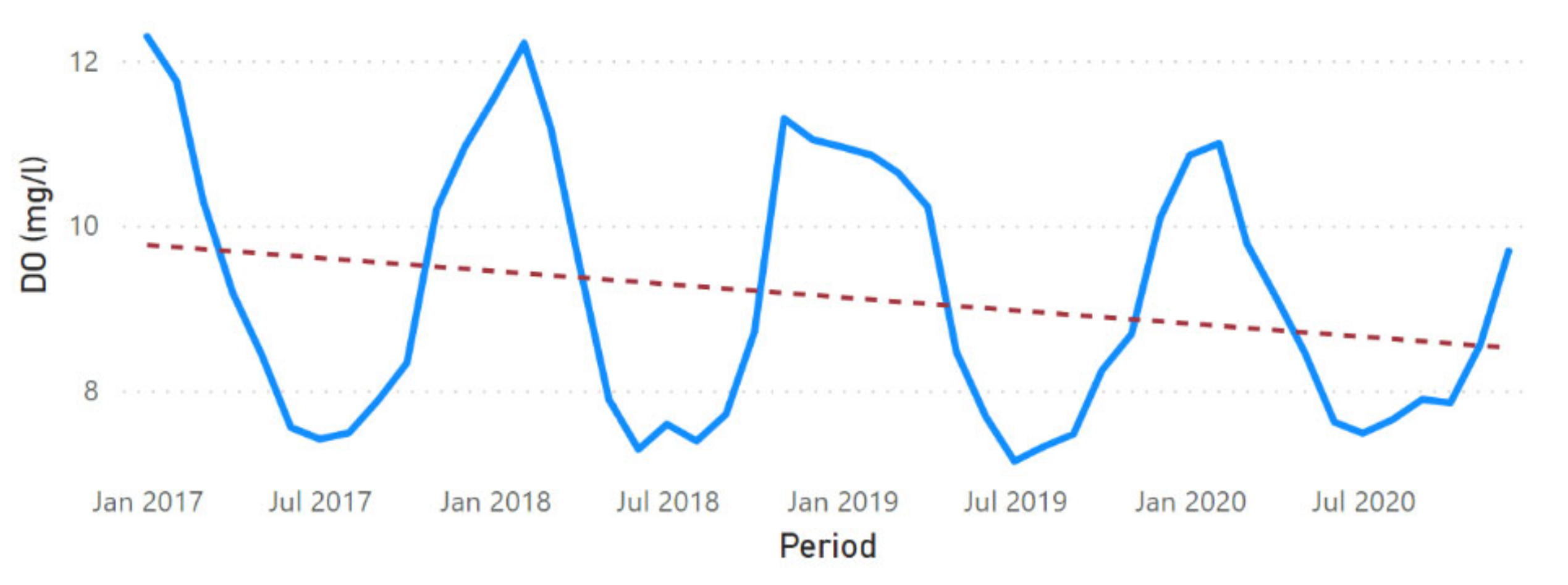
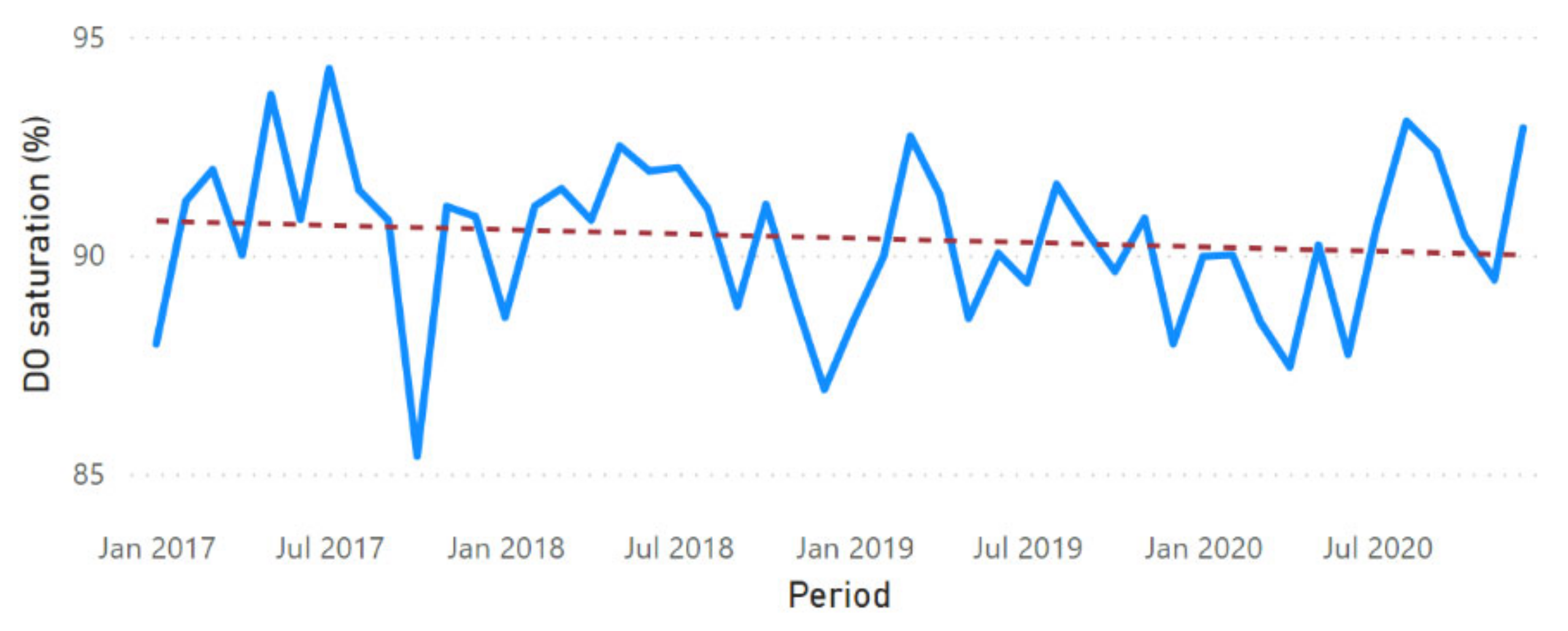
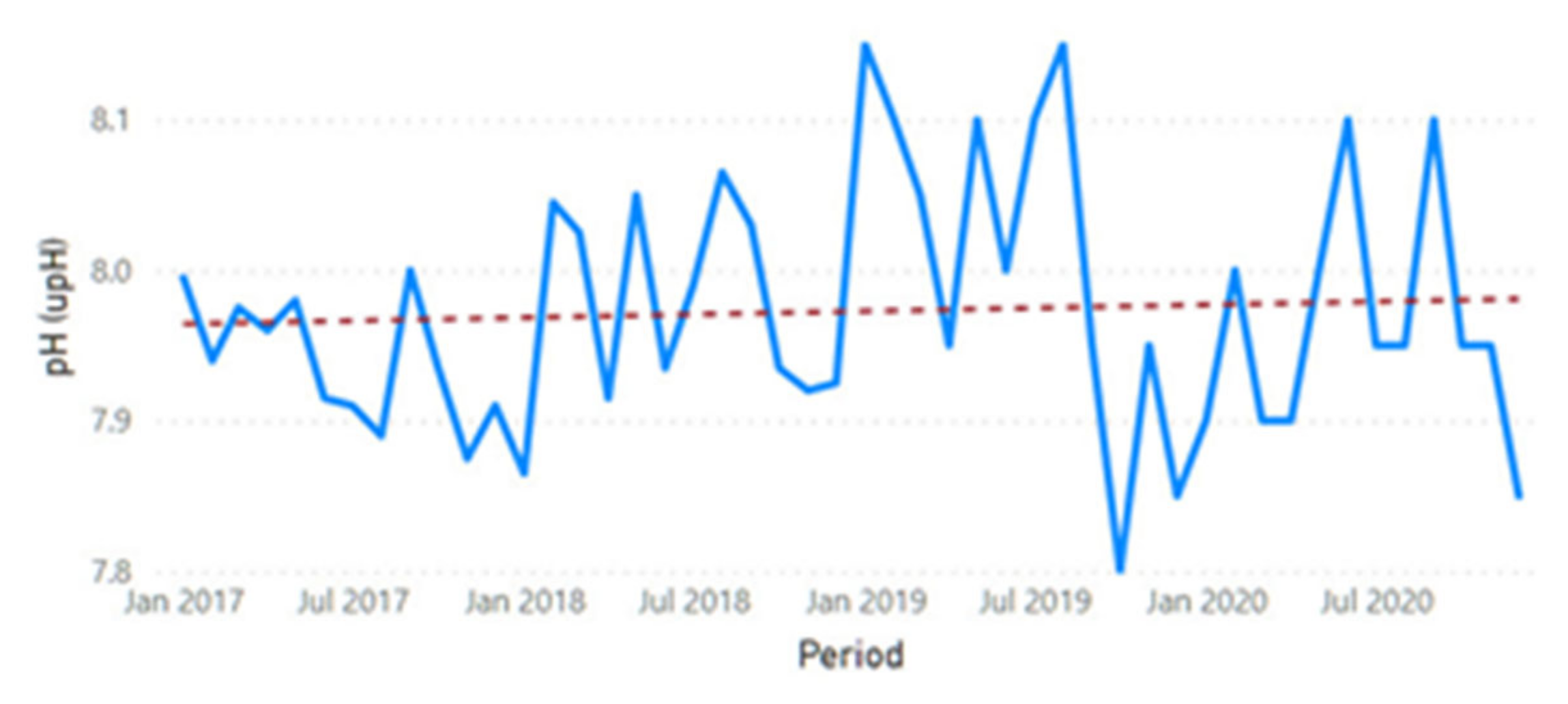
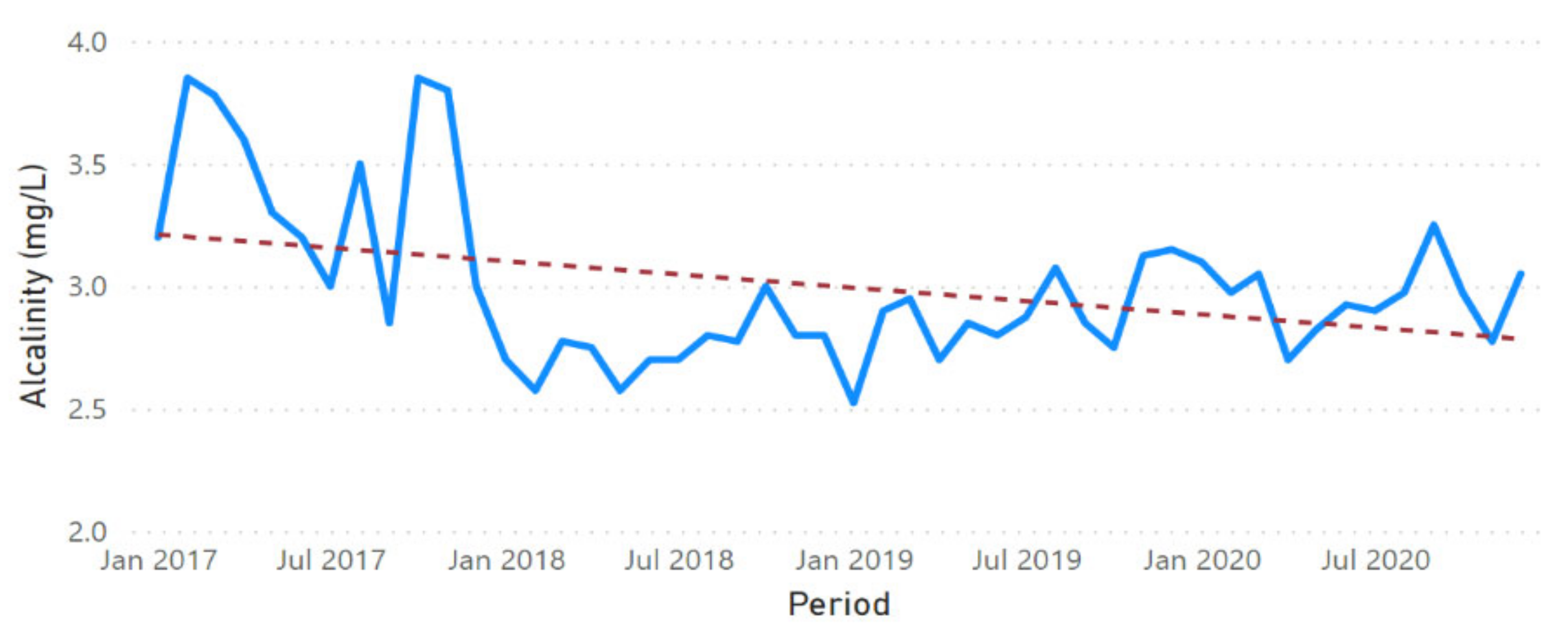
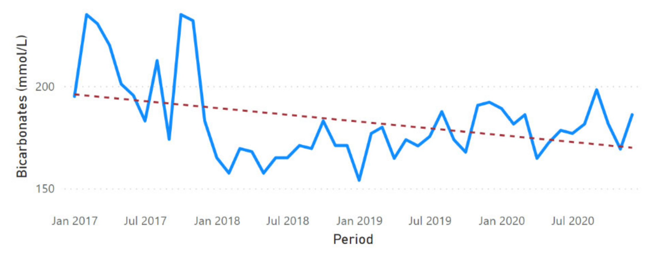
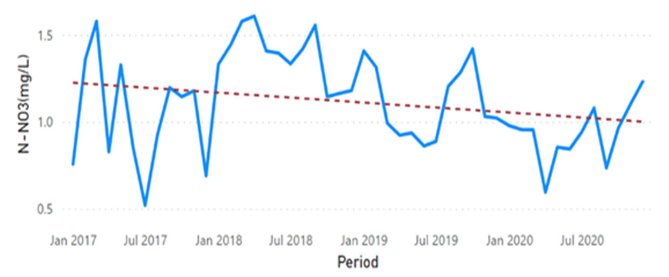
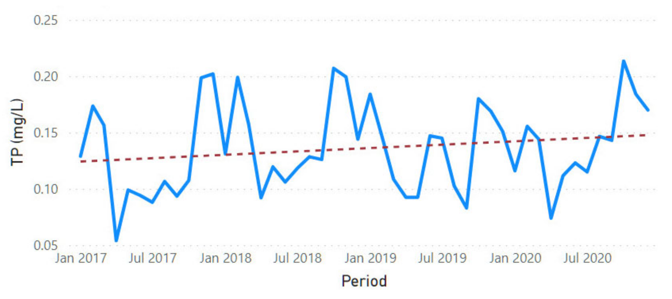
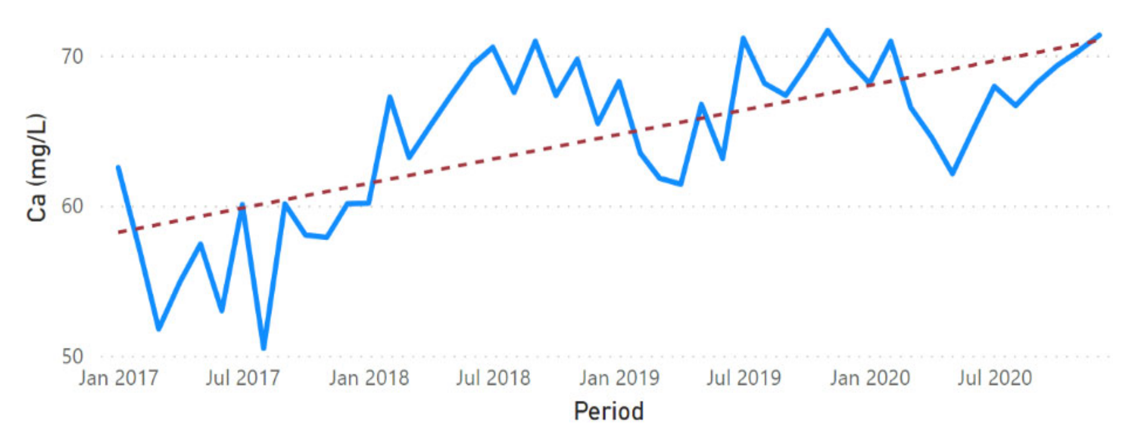
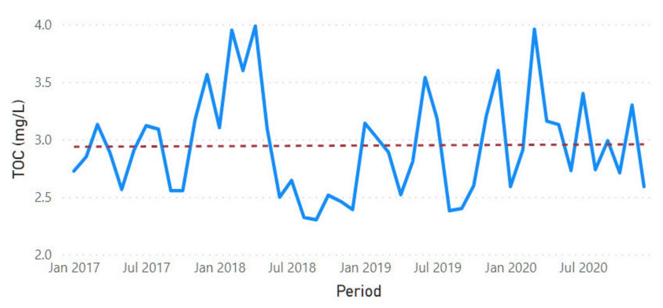
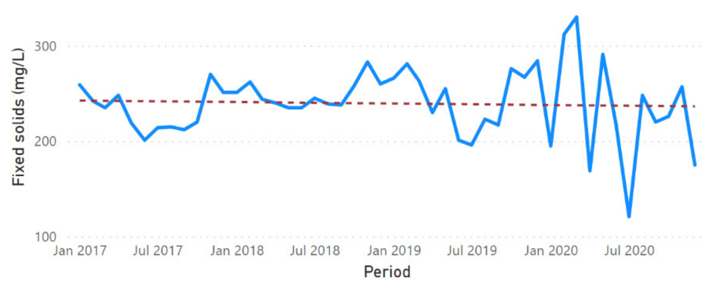
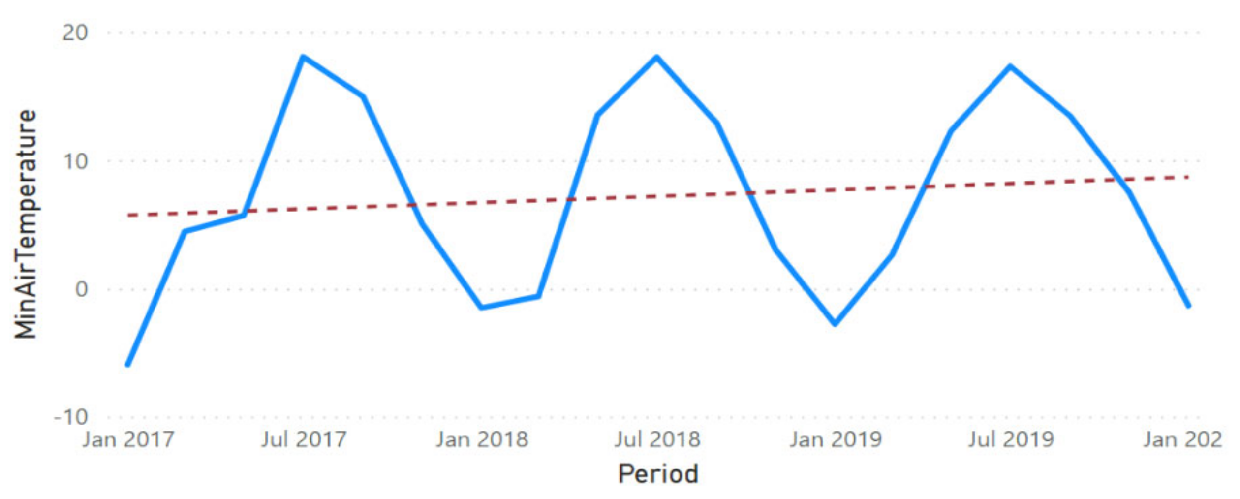
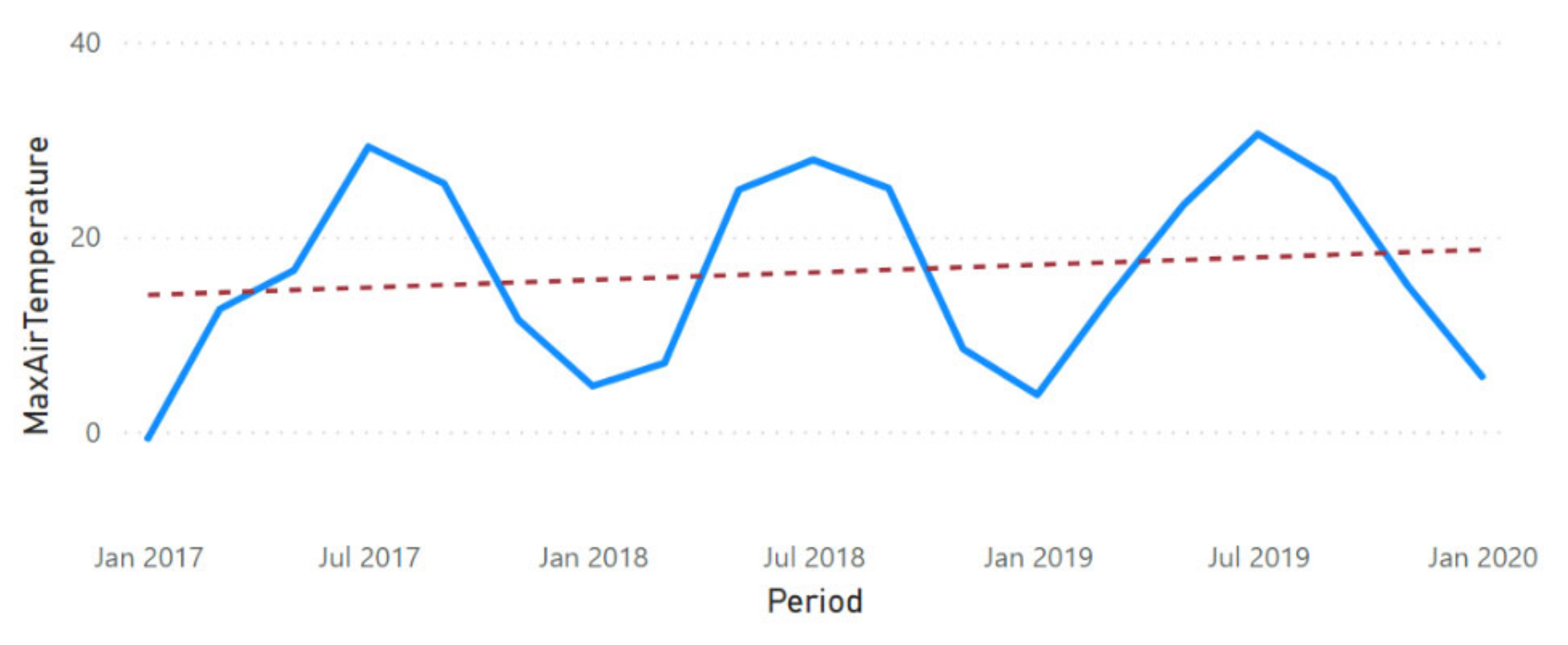
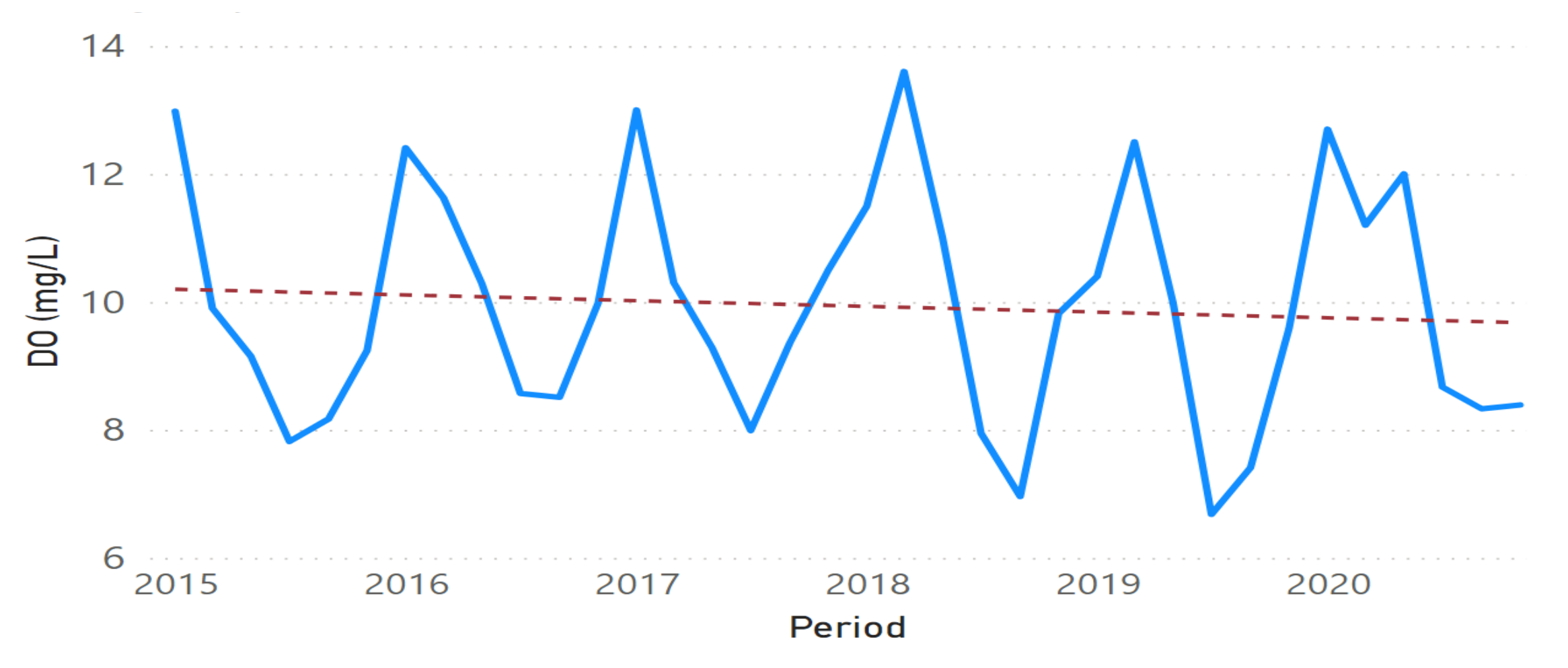
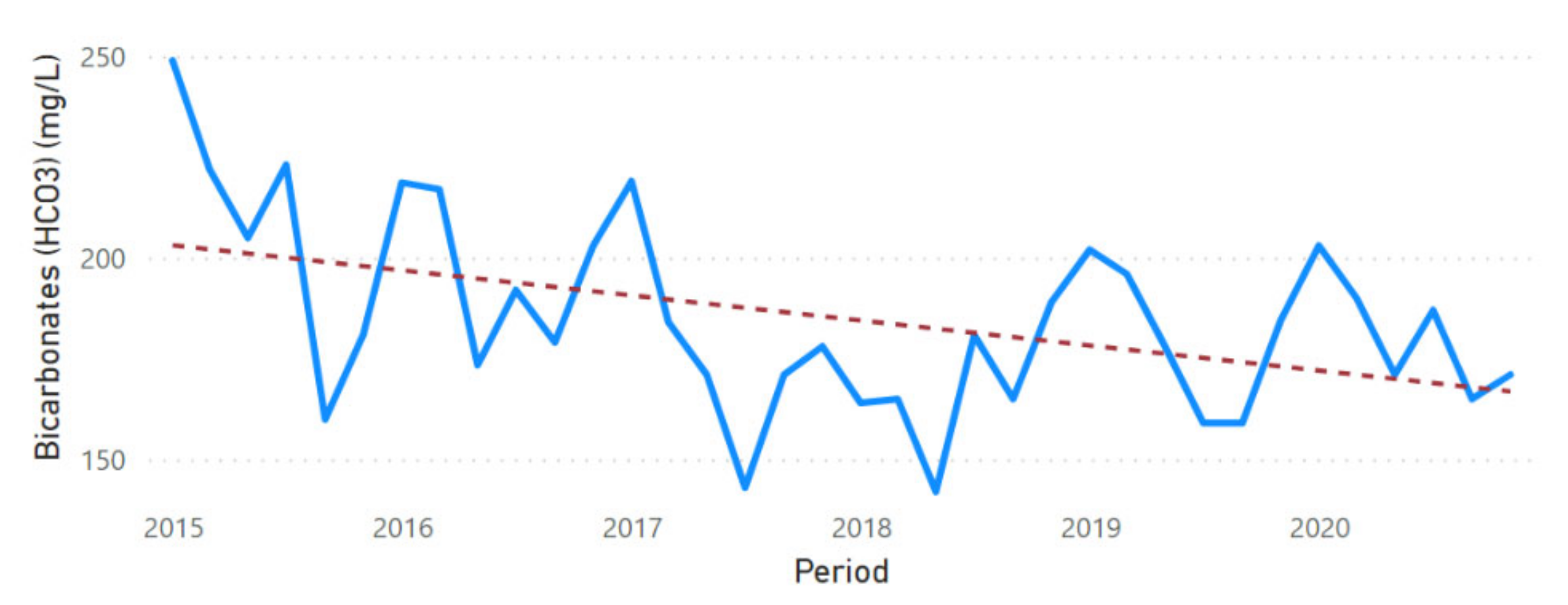
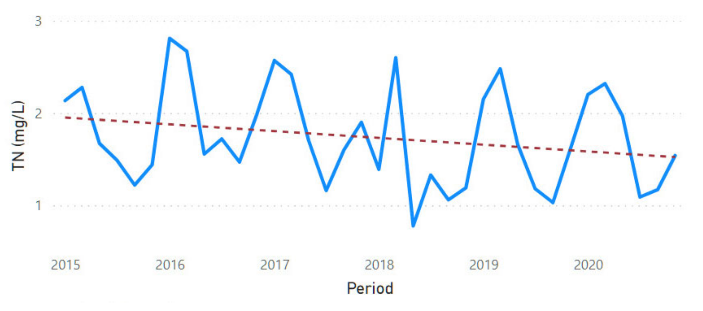
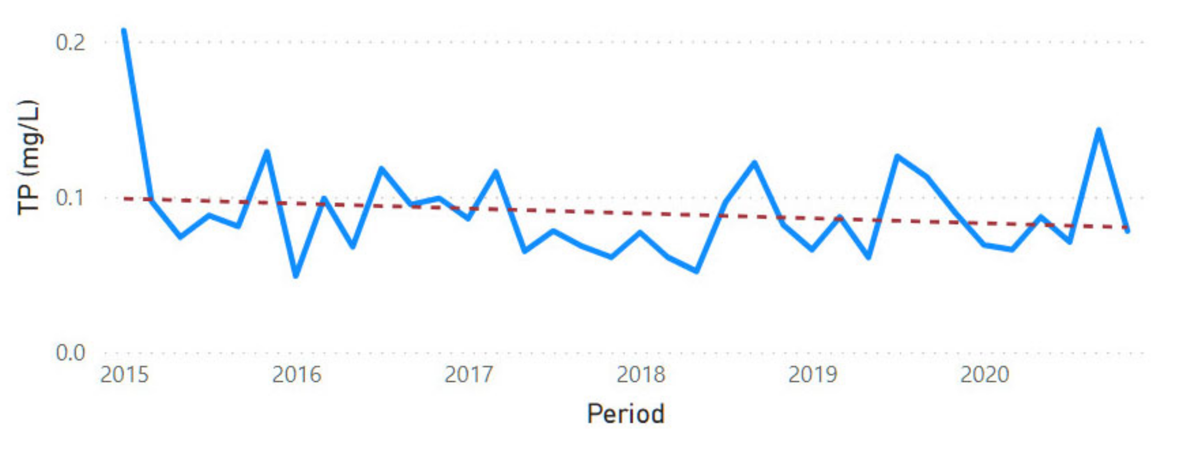
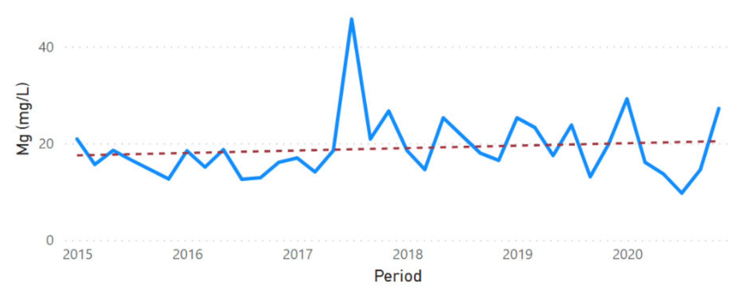
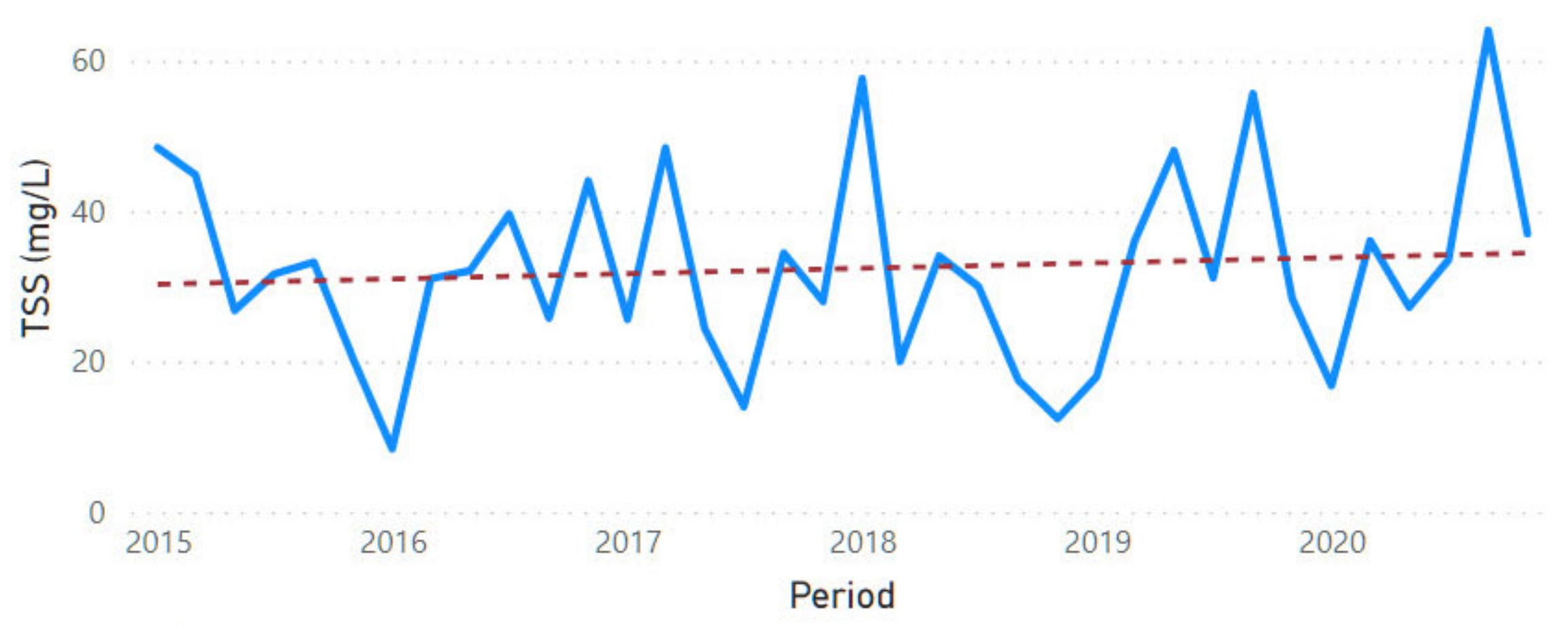
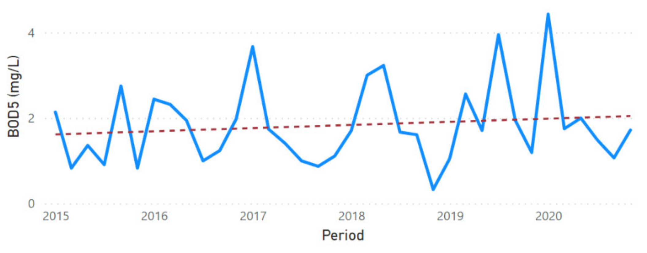
3.2. Physicochemical Parameter Trend Lines

The physicochemical parameters were monitored monthly during a 4-year period in Galați county and once every 2 months during a 6-year period at the Tulcea county sampling point, as presented in Figure 1. The registered results were analyzed to determine the trend lines and used to establish multi-linear regression (MLR) models and forecast analysis. Therefore, in the case of the Galați county sampling point, the recorded data for the air temperature was divided into two groups: maximum air temperature and minimum air temperature. The trend lines of both groups revealed a clear upward dynamic (Figure A1 and Figure A2) from 2017 until 2020. Thus, the data revealed that the maximum air temperature increased by 7.06% during the hot season and by 23.28% during the cold season within the analyzed period. Additionally, the minimum air temperature recorded a higher increase, being 8.11% during the hot season and 109.5% during the cold season. The upward trend line in the air temperature caused the increase in the water temperature, something also revealed in the Danube River Galați sampling point (Figure A3). Thus, in the hot season, the water temperature registered a 0.79% increase, while in the cold season, a 30.95% increase was recorded during the analyzed period. Additionally, the water DO and DO saturation presented a decreasing trend line (Figure A4 and Figure A5), a situation which was correlated with the upward trend lines associated with the air and water temperatures (Figure A1, Figure A2 and Figure A3). Other authors revealed that an increase in the surface temperature leads to an outgassing of oxygen from the ocean and a reduction in the surface water oxygen concentration [89]. The pH trend line (Figure A6) registered a decreasing trend line of 0.27% during the analyzed period, thus confirming the findings reported by other authors [90] related to an inverse pH response to temperature variations. The pH dynamics were sustained by both the water alkalinity and bicarbonate concentration trend lines, which revealed a decreasing trend (Figure A7 and Figure A8). The nitrite-nitrogen, ammonium-nitrogen and total nitrogen registered an upward trend (Figure A10, Figure A11 and Figure A12), while nitrate registered a decrease (Figure A9). However, there are studies which predicted an increase in the nitrate concertation as well as an increase in the rate of mineralization linked to the increase in temperature [91]. This scenario was confirmed by the significant upward trend lines registered for TP, Mg and Ca (Figure A13, Figure A14 and Figure A15). However, the turbidity and TSS (Figure A16 and Figure A17) trend lines revealed a decreasing tendency, while the TOC trend line presented a small increase (Figure A18). In addition, the BOD5 and fixed solids trend lines indicated a relatively stable dynamic for these parameters (Figure A19 and Figure A20). This may have been due to the high water flow of Danube River and, therefore, its capacity to transport solids and organic matter, revealing the river’s auto-epuration capacity. At the Tulcea county sampling point, the trend lines for both the maximum and minimum air temperature revealed a clear upward dynamic (Figure A21 and Figure A22) from 2017 to 2020. Thus, the data revealed that the maximum air temperature increased by 9.27% during the hot season and by 19.07% during the cold season in the analyzed period. Additionally, the minimum air temperature recorded a higher increase, being 7.45% during the hot season and 44.65% during the cold season. Therefore, the Galati sampling point was exposed to a more aggressive climate change impact when considering the air temperature trend lines (Figure A1, Figure A2, Figure A21 and Figure A22). In addition, the water temperature revealed an upward trend line (Figure A23) with a 30.11% increase during the cold season, while the DO presented a decreasing trend line (Figure A24). The pH trend line (Figure A25) revealed a decreasing trend line, being 1.30% during the analyzed period. This can be due to sediments and therefore organic matter deposits, which accumulate more in Tulcea compared with the Galați sampling area due to the geographic position of this sampling point (i.e., closer to Danube Delta). Both the water alkalinity and bicarbonate concentration trend lines revealed a decreasing trend (Figure A26 and Figure A27) of 12.29% and 12.33%, respectively, during the analyzed period.

The total water nitrogen and nitrate-nitrogen at the Tulcea sampling point revealed a decreasing trend line, whereas the nitrite-nitrogen recorded a relatively constant trend (Figure A31, Figure A28 and Figure A29), and the ammonium-nitrogen (Figure A30) registered the only upward trend among the nitrogen compounds analyzed in present study. This could indicate a relatively better ecological status in the Tulcea sampling area, mostly due to lower climate change impact revealed by the air temperature trend line compared with the Galați sampling point. This can be confirmed by the decreasing trend lines registered for TP and Ca (Figure A32 and Figure A34) and the small increasing trend of Mg compared with the Galați sampling station. The TSS and BOD5 revealed upward trend lines (Figure A35 and Figure A36), the evolution of which supports the scenarios of a superior solids accumulation rate in Tulcea compared with the Galați sampling point.

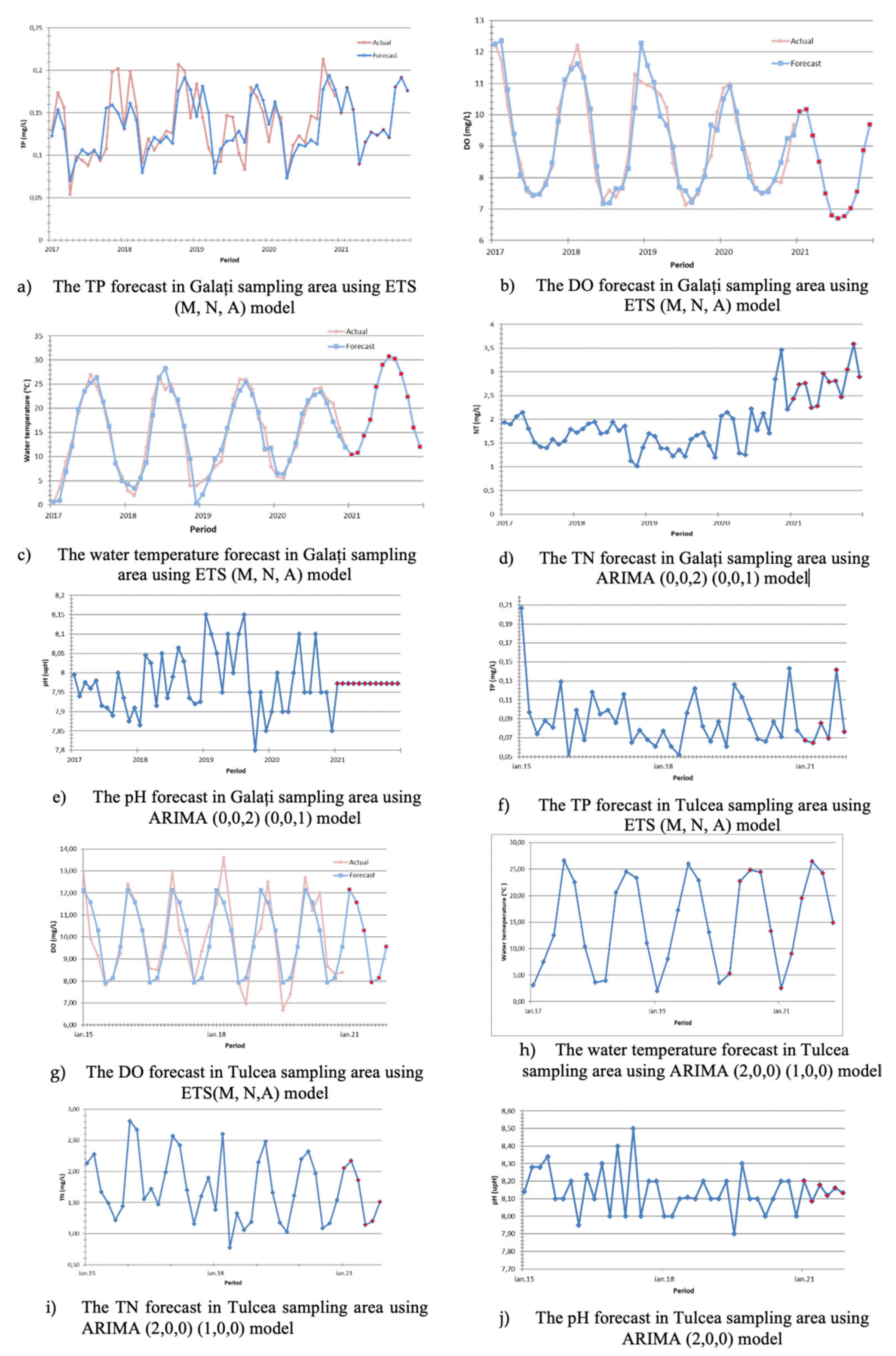
3.3. Physicochemical Parameter Forecast Analysis

To perform the forecast analysis for both the Galați and Tulcea sampling points, five physicochemical parameters were analyzed: the TN, TP, water temperature, pH and dissolved oxygen concentration. The parameters were considered as the most suggestive to characterize the analyzed area status in relation to climate change, a fact confirmed by their trend line evolutions (Figure A3, Figure A4, Figure A12, Figure A13, Figure A24, Figure A25, Figure A31 and Figure A32). Therefore, the TP forecast in the Galați sampling area was performed by applying the ETS (M, N, A) model (Figure 2a), which was selected by considering the Akaike coefficient. EST Smoothing is a multiplicative error model without trends and with additive seasonality. The model keeps its oscillating trend for the forecasted period, obtaining values close to those that were used in determining the model (Figure 2a). The forecasted average concentration of the TP in water for the year 2021 was 2.41% higher compared with the 2020 average and 6.47% higher than the 2017–2020 period’s average. For the DO forecast, an ETS (M, N, M) multiplicative errors model (Figure 2b) was selected without trends and with multiplicative seasonality. The model (Figure 2b) revealed that the dynamics of DO would register the same oscillation for the forecasted period, but with a slightly significant decrease compared with the current values for July and August. The forecasted average concentration of the DO in water for 2021 was 6.56% lower compared with the 2020 average and 9.78 % lower than the 2017–2020 period’s average. For the water temperature forecast, an ETS (A, N, A) additive model without trends and with additive seasonality was applied (Figure 2c). The time series maintained its oscillating trend during the year due to the seasons that demanded seasonality on the series. For the summer months, higher forecasted values were obtained compared with the actual values (Figure 2c), emphasizing the future global warming effect on the water DO at the Galați sampling point. The forecasted average value of the water temperature for 2021 was 28.71% higher compared with the year 2020 average and 37.92% higher than the 2017–2020 period’s average. The TN and pH forecast analysis were performed by using a Seasonal Autoregressive Integrated Moving Average (SARIMA) model (Figure 2d,e), since the seasonality characteristic of the forecasted variable existed. SARIMA is considered a method of predicting univariate time series that contain trends and seasonality. The forecasted average value of pH in the water for 2021 was 0.12% higher compared with the average pertaining to the year 2020 and 0.007% lower than the 2017–2020 time period’s average. Additionally, the forecasted average concentration of the TN in the water for the year 2021 was 30.72% higher compared with the 2020 average and 57.99% higher than the 2017–2020 time period’s average. The TP forecast in the Tulcea sampling area was performed by applying the ARIMA seasonal model (1,0,1) (0,0,1) (Figure 2f). This model considers the first gap as well as the first delay of the trend side. The estimated series continued its oscillating evolution, having actual values like the previous ones. The forecasted average concentration of the TP in the water for 2021 was 0.09% higher compared with the 2020 average and 0.03% higher than the 2017–2020 time period’s average.

For the DO forecast, an ETS (M, N, A) multiplicative error model (Figure 2f) without trends and with additive seasonality was selected. Noticeably (Figure 2g), the predicted values had the same tendency as those used for training. The series would keep its oscillating trend for the next period. The average concentration of the DO in the water forecasted for 2021 was 2.70% lower than that for the 2020 average and 0.01% lower than the 2017–2020 time period’s average. For the water temperature forecast (Figure 2h), an ARIMA (2,0,0) (1,0,0) seasonal model was applied. The forecasted average value of the water temperature for the year 2021 was 2.62% higher compared with the 2020 average and 9.39% higher than the 2017–2020 time period’s average. The TN forecast analysis was performed by using an ARIMA seasonal model (2,0,0) (1,0,0) (Figure 2i) which was autoregressive for both the trend and the season. The estimated data revealed that the variable would keep its oscillations given by the seasons. Furthermore, the forecasted average concentration of the TN in the water for 2021 was 3.44% lower compared with the 2020 average and 4.68% lower than the 2017–2020 time period’s average. The pH forecast analysis was performed by using a second-order autoregressive model; thus, the current value of the water pH depended on two previous moments (lags). From the analysis of the forecasted data (Figure 2j), very small oscillations could be observed for the next period. The forecasted average value of the pH in the water for 2021 was 0.57% higher compared with the 2020 average and 0.04% higher than the 2017–2020 time period’s average.

3.4. Physicochemical Parameter Multiple Linear Regression (MLR) Models

Ten MLR models were identified after processing the physicochemical parameter dataset. Therefore, for each of the sampling areas (Tulcea and Galați), five MLR models for determining the P-PO₄, N-NO₃, N-NO₂, N-NH₄ and SO₄ dependent variables were elaborated (

Table 3. Physicochemical parameters of the Multiple Linear Regression (MLR) models recorded for the Galați and Tulcea study sectors.

Sampling Point	MLR Prediction Model	Model No.
Galati	P-PO4 = −2.918 − 0.276 SO4 + 1.162 Bicarbonates + 0.457 N-NO3 + 0.8701 TP + 0.095 water level	M1
	N-NO3 = -3.818 + 0.514 EC + 1.051 Mg + 0.401 SO4 − 0.166 N-NO2 + 1.047 NT	M2
	N-NO2 = −5.285 − 0.378 DO + 1.618 Mg + 0.497 SO4 − 0.775 N-NO3 + 1.277 NT + 0.313 water level	M3
	N-NH4 = -6.077 + 0.557 TSS + 0.667 Mg + 0.772 Chloride + 1.004 Bicarbonates	M4
	SO4 = 3.523 + 0.701 COD − 0.987 Ca − 0.614 Mg + 0.588 N-NO3 − 0.386 NT	M5
Tulcea	P-PO4 = 3.010 + 3.344 DO − 0.671 BOD5 + 0.275 N-NH4 + 0.605 N-NO2 − 0.776 N-NO3 + 0.472 TP − 0.402 TSS − 0.426 FS + 0.819 Mg − 1.975 TH − 1.254 Cl − 0.860 SO4	M6
	N-NO3 = −0.178 + 0.940 TN	M7
	N-NO2 = 1.340 − 6.920 pH + 0.992 EC − 2.787 DO − 0.240 COD + 0.5887 BOD5 − 0.237 N-NH4 + 0.650 N-NO3 + 0.227 P-PO4 + 0.2435 TSS + 0.3081 FS − 0.694 Mg + 1.391 TH + 0.648 Chloride + 0.669 SO4	M8
	N-NH4 = 2.080 − 17.370 pH + 4.430 EC − 7.310 DO − 0.780 COD + 1.492 BOD5 − 1.785 N-NO2 + 1.520 N-NO3 + 0.541 P-PO4 + 0.548 TSS + 0.906 FS − 1.658 Mg + 3.168 TH + 1.608 SO4	M9
	SO4 = −1.430 + 4.690 pH + 2.667 DO − 0.511 BOD5 + 0.213 N-NH4 + 0.643 N-NO2 − 0.644 N-NO3 − 0.318 P-PO4 − 0.275 TSS − 0.324 FS + 0.723 Mg − 1.389 TH − 0.891 Cl	M10

). All variables used within the models had p-values < 0.05.

The first MLR model (M1) (Table 3) determined the concentration of P-PO₄ in the Danube River’s water at the Galați sampling area based on the bicarbonates, water level, TP, SO₄ and N-NO₃ recorded values. The model explained 81.40% of the variance of P-PO₄ in the water. Additionally, the value of the predicted R-sq was close to the R-sq value, indicating good model performance. Additionally, the S-value was low, indicating that the model achieved the best degree of precision. The coded coefficients permitted us to identify the variable with the largest impact on the model response. Thus, for M1, the bicarbonate value had the strongest influence on the resulting concentration of P-PO₄ in the water, followed by TP and N-NO₃. The second MLR model (M2) determined the concentration of N-NO₃ in the Danube River’s water at the Galați sampling area based on the EC, Mg, SO₄, N-NO₂ and NT recorded values (Table 3). The model explained 85.79% of the variance of N-NO3 in the water. The model had good performance, and the S-value was low, indicating the best performance and degree of precision. Therefore, for M2, the values of Mg and NT had the strongest influence on the resulting concentration of N-NO₃ in the water, followed by EC and SO₄. The third model (M3) determined the concentration of N-NO₂ in the Danube River’s water at the Galați sampling area based on the DO, Mg, SO₄, NT, water level and N-NO₃ concentrations (Table 3). The model explained 73.25% of the variance of N-NO₂ in the water. The model indicated good performance (the predicted R-sq value was close to R-sq), a situation also revealed by the low S-value, which indicated a high degree of precision. By analyzing the coded coefficients of the third model, it can be stated that the values of Mg, NT and N-NO₃ had the strongest influence on the resulting concentration of N-NO₂ in the Danube River’s water at the Galați sampling area. The fourth model (M4) determined the concentration of N-NH₄ within the Danube River’s water at the Galați sampling area based on the TSS, Mg, chloride and bicarbonate concentrations (Table 3). The model explained 69.52% of the variance of N-NH₄ in the water. The low S-value indicated a high degree of precision. By analyzing the coded coefficients of M4, it can be stated that the values of the bicarbonate and chloride concentrations had the most significant impact over the dependent variable. The fifth model (M5) determined the concentration of SO₄ in the Danube River’s water at the Galați sampling area based on the concentrations of Ca, COD, Mg, N-NO₃ and NT (Table 3). The model explained 71.55% of the variance of SO₄ in the water. The model indicated good performance (the predicted R-sq value was close to R-sq), and the situation also revealed through a relatively low S-value that it had good precision. By analyzing the coded coefficients of the fifth model, it can be stated that Ca had the most significant impact over the dependent variable, followed by COD, Mg and N-NO₃. The sixth model (M6) determined the concentration of P-PO₄ within the Danube River’s water at the Tulcea sampling area based on the DO, BOD5, N-NH₄, N-NO₂, N-NO₃, TP, TSS, FS, Mg, TH, chloride and SO₄ concentrations (Table 3). The model explained 61.80% of the variance of P-PO₄ in the water. The model indicated good performance (the predicted R-sq value was close to R-sq), and the situation also revealed through a low S-value that it had a high degree of precision. By analyzing the coded coefficients of the sixth model, it can be stated that the DO, TH, chloride, SO₄ and N-NO₃ had the most significant impact on the dependent variable. The seventh MLR model (M7) determined the concentration of N-NO₃ within the Danube River’s water at the Tulcea sampling area based on the TN concentration (Table 3). The model explained 71.52% of the variance of N-NO₃ in the water. The model indicated very good performance (the predicted R-sq value was close to R-sq), and the situation also revealed through a low S-value that it had a considerably high degree of precision. The values of the coded coefficients presented for the seventh model indicated a significant impact from the TN variation over the dependent variable. The eighth MLR model (M8) determined the concentration of N-NO₂ within the Danube River’s water at the Tulcea sampling area based on the pH, EC, DO, COD, BOD5, N-NH₄, N-NO₃, P-PO₄, TSS, FS, Mg, TH, chloride and SO₄ concentrations (Table 3). The model explained 81.83% of the variance of N-NO₂ in the water. When considering the predicted R-sq value, the R-sq and the S-value, it can be stated that M8 had a high degree of precision. The coded coefficients revealed that the pH, DO and TH had the most significant impact on the dependent variable.

The ninth model (M9) determined the concentration of N-NH₄ in the Danube River’s water at the Tulcea sampling area based on the pH, EC, DO, COD, BOD5, N-NO₂, N-NO₃, P-PO₄, TSS, FS, Mg, TH and SO₄ concentrations (Table 3). The model explained 75.12% of the variance of N-NH₄ in the water. Additionally, the value of the predicted R-sq was close to the R-sq value, indicating good model performance. However, the S-value was high, indicating that the model did not achieve the best degree of precision. The coded coefficients permitted us to identify the variable with the largest impact on the model’s response. By analyzing the coded coefficients of the ninth model, it can be stated that the values of the pH, DO, EC, TH, N-NO₃, N-NO₂, Mg and SO₄ concentrations had the most significant impact over the dependent variable. The last MLR model (M10) determined the concentration of SO₄ in the Danube River’s water at the Tulcea sampling area based on the pH, DO, BOD5, N-NH₄, N-NO₂, N-NO₃, N-NH₄, TSS, FS, Mg, TH and chloride concentrations. The model explained 75.36% of the variance of SO₄ in the water. The model indicated good performance (the predicted R-sq value was close to the R-sq value), a situation also revealed by the low S-value that indicated a high degree of precision. By analyzing the coded coefficients of M10 (Table 3), it can be stated that the values of the pH, DO, TH and chloride concentrations had the strongest influence on the resulting concentration of SO₄ in the Danube River’s water at the Tulcea sampling area.

Positive correlation (Pearson and Spearman coefficients) was highlighted in the study of Kovač et al. (2016) in an aquifer from Zagreb between the nitrate concentrations and the levels of DO due to the high nitrate mobility in aerobic conditions [92]. Furthermore, water EC values are associated with high nitrate concentrations due to low precipitation [93]. Other authors [94] conducted a study where they performed linear regression analysis between the EC values and nitrate concentrations in soil samples from Tsukuba, Japan, and they highlighted the positive correlation between the two variables.

It is well known that under the conditions of low DO values, the maximum conversion of ammonia to nitrite is achieved [95,96].

The positive correlation between ammonium and suspended solids has been previously elucidated in the estuary waters of the Gulf of Mexico [97].

The presence of PO₄ in water systems indirectly influences the concentration of DO by stimulating the rapid development of microalgae (through algal blooms) which consume the DO [98].

According to other authors [99], increased DO levels in water inhibit NO₂⁻ oxidation rates. Additionally, it has been pointed out that species of nitrite are stable at a pH of 7 and 10.6 (NO₂⁻), while unstable species (HNO₂) are formed at lower pH values (2.5) [100]. Furthermore, pH is one of the key factors for controlling the NH₄⁺ content in surface waters, and low pH values can increase the ammonium content [101].

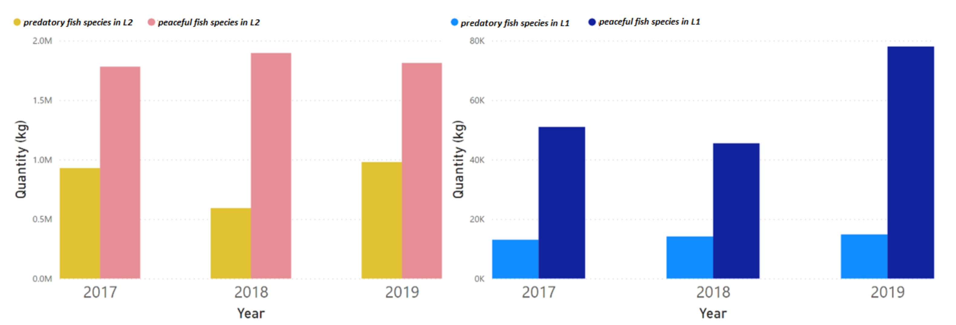
3.5. Multiple Linear Regression (MLR) Models Based on the Fish Catch Dataset for the L1 and L2 Study Area

To develop an efficient toll for BE resilience, based on the evaluation of fish stocks from the L1 and L2 study regions, presented in Figure 1, MLR predicting methods were used based on the existing fish catch dataset. Therefore, 23 models were elaborated, with 13 of them having applicability in the L1 while the other 10 in were in the L2 study region (

Table 4. Multiple Linear Regression (MLR) models based on the fish catch dataset for the L1 and L2 study areas.

Study Area	MLR Prediction Model	Model No.
L1	Ccp = −0.413 + 0.350 Pcp + 0.2316 Wbr + 0.607 Ctf	L1M1
	Pcp = −0.182 + 1.0377 Fbr	L1M2
	Fbr = 0.289 + 0.6836 Pcp + 0.2827 PkPrc	L1M3
	Vmb = 0.256 + 0.780 Psh	L1M4
	Cbb = 0.688 + 0.783 PkPrc	L1M5
	Rch = −0.198 + 0.4816 Pcp + 0.452 Wbr	L1M6
	Wbr = 0.202 + 0.375 Vmb + 0.926 Rch − 0.447 Asp	L1M7
	Asp = −0.010 + 0.9502 PkPrc	L1M8
	Ctf = 0.385 + 0.6213 Ccp + 0.748 PkPrc − 0.3336 Pk − 0.2185 Psh	L1M9
	PhPrc = −0.003 + 0.370 Asp + 0.475 Ctf + 0.2058 Pk	L1M10
	Pk = 1.007 + 0.754 Rch + 1.037 PkPrc − 1.159 Ocp	L1M11
	Ocp = 0.346 + 0.335 Rch + 0.365 Ctf − 0.3086 Pk + 0.449 Psh	L1M12
	Psh= 0.243 + 0.3145 Vmb + 0.7288 Ocp	L1M13
L2	Fbr = −3745 − 1.258 Pk + 1.906 Rch + 2.188 PkPrc	L2M1
	Pcp = 10049 + 7.092 Rch − 1.970 PkPrc	L2M2
	Ocp = −2419 + 0.1091 Fbr + 0.700 Ccp	L2M3
	Ccp = 231 + 0.364 Ocp + 0.798 Ctf − 0.1683 PkPrc	L2M4
	Pk = −2032 − 0.1722 Fbr + 0.0290 Pcp + 0.725 Rch + 1.503 Tnch	L2M5
	Rch = 1391 + 0.1286 Fbr + 0.0752 Pcp + 0.2934 Pk	L2M6
	Ctf = 3003 + 0.6943 Ccp + 0.2869 Pk − 1.215 Tnch	L2M7
	Tnch = 2746 + 0.0794 Ocp + 0.1264 Pk − 0.1522 Ctf	L2M8
	Prc = 1259 + 0.1830 Rch	L2M9
	PkPrc = −643 + 0.2382 Fbr	L2M10

).

Thus, the first model (L1M1) helped to predict common carp fish stocks based on Prussian carp, catfish and white bream stocks. The model explained 94.94% of the variance of the common carp stocks within the L1 study area. The model indicated good performance (the predicted R-sq value was close to the R-sq value) and revealed that the catfish and Prussian carp statuses had the strongest influence on the common carp stocks in the L1 study area (Table 4). The second model (L1M2) predicted Prussian carp stocks based on the freshwater bream stocks within the L1 study area. The model explained 95.51% of the variance of Prussian carp stocks in L1. The model indicated good performance (the predicted R-sq value (94.82%) was close to the R-sq value) and revealed that the situation of Prussian carp stocks was strongly influenced by the freshwater bream in L2 (Table 4). The third model (L1M3) confirmed the interspecies fish relationship presented in previous models and predicted the freshwater bream stocks in L1 based on Prussian carp and pikeperch stocks. The model explained 97.37% of the variance of freshwater bream stocks in L1. The model indicated good performance (the predicted R-sq value (96.61%) was close to the R-sq value) and confirmed the strong relation between the freshwater bream stocks and Prussian carp as the main independent variable of L1M3 (Table 4). The fourth model (L1M4) predicted the vimba stocks based on the Pontic shad stocks in L1. The model explained 58.81% of the variance of vimba stocks in L1. Additionally, the value of the predicted R-sq was further from the R-sq value, and the S-value was high, indicating that the model did not achieve the best degree of prediction and precision. However, the coded coefficient revealed the significant contribution of the Pontic shad independent variable in the prediction of the vimba dependent variable (Table 4). The fifth model (L1M5) predicted the common barbel stocks based on the pikeperch in L1. The model explained 42.56% of the variance of common barbel stocks in L1. Additionally, the value of the predicted R-sq was close to the R-sq value, and the S-value was relatively low, a situation that indicated that L1M5 did achieve an acceptable degree of prediction and precision. The coded coefficient analysis revealed the significant contribution of the pikeperch independent variable in the prediction of the common barbel dependent variable (Table 4). The sixth model (L1M6) predicted the roach stocks in L1 based on the Prussian carp and white bream stocks. The model explained 86.13% of the variance of roach stocks in L1. The model indicated good performance (the predicted R-sq value (79.81%) was close to the R-sq value) and revealed that the situation of the roach stocks was strongly influenced by both the Prussian carp and white bream stocks in an almost equal manner (Table 4). The seventh model (L1M7) predicted the white bream stocks in L1 based on the vimba, roach and asp stocks. The model explained 79.99% of the variance of white bream in L1. The model indicated good performance (the predicted R-sq value (69.28%) was relatively close to the R-sq value) and revealed that the status of the white bream stocks was mostly influenced by the roach stock followed by the asp stock, as revealed by the coded coefficient analysis (Table 4). The eighth model (L1M8) predicted the asp stocks in L1 based on the pikeperch stocks. The model explained 88.99% of the variance of asp stocks in L1. Additionally, the value of the predicted R-sq (86.90%) was close to the R-sq value, indicating that M18 did achieve a good degree of prediction and precision. The coded coefficient analysis revealed the significant contribution of the pikeperch independent variable in the prediction of the asp dependent variable (Table 4). The ninth model (L1M9) predicted the catfish stocks in L1 based on the common carp, pikeperch, pike and Pontic shad stocks. The model explained 97.15% of the variance of catfish stocks in L1. The model indicated good performance (the predicted R-sq value (92.50%) was close to the R-sq value), and the coded coefficient analysis revealed the significant contribution of the common carp and pikeperch independent variables in the prediction of the catfish dependent variable (Table 4). The tenth model (L1M10) predicted the pikeperch stocks in L1 based on the asp, catfish and pike stocks. The model explained 95.05% of the variance of pikeperch stocks in L1. However, the model indicated relatively good performance (the predicted R-sq value (88.29%) was close to the R-sq value), and the coded coefficient analysis revealed that catfish and asp contributed the most to the pikeperch prediction model (Table 4). The eleventh model (L1M11) predicted the pike stocks in L1 based on the roach and pike stocks and other cyprinid species, which were recorded as a different category in the reported catches. The model explained 78.24% of the variance of pike stocks in L1. Additionally, the value of the predicted R-sq was close to the R-sq value, and the S-value was relatively low, a situation indicating that L1M11 did achieve an acceptable degree of prediction and precision. The coded coefficient analysis revealed the significant contribution of pikeperch and the other cyprinid category in the prediction of the pike dependent variable (Table 4). The category of other cyprinids was composed of all cyprinid species recorded as catches, except for the cyprinid species considered a separate group in the present analytical framework. Therefore, the twelfth model (L1M12) predicted the other cyprinid stocks in L1 based on the roach, catfish, pike and Pontic shad stocks. The model explained 92.74% of the variance of the other cyprinids group in L1. Additionally, the value of the predicted R-sq was close to the R-sq value, and the S-value was relatively low, a situation indicating that L1M12 did achieve an acceptable degree of prediction and precision. The coded coefficient analysis revealed an almost equal contribution by the roach, catfish, pike and Pontic shad stocks in the prediction of the other cyprinids dependent variable. The last MLR model (L1M13) for fish stock prediction in L1 targeted the prediction of the Pontic shad stocks based on vimba and also other members of the cyprinids group. The model explained 90.00% of the variance of the Pontic shad stocks in L1. The model indicated good performance (the predicted R-sq value (88.25%) was close to the R-sq value), and the coded coefficient analysis revealed the significant contribution of the other cyprinids group in the prediction of the Pontic shad dependent variable (Table 4).

The analysis of the fish stock dataset from the L2 sampling area revealed 10 MLR prediction models (Table 4). Therefore, the first model (L2M1) generated predictions for the freshwater bream stocks within the L2 study area based on the pike, roach and pikeperch stocks. The model explained 88.88% of the variance of freshwater bream stocks in L2. Additionally, the predicted R-sq value was relatively far from the R-sq value, and the S-value was high. This indicates that L2M1 did not achieve the best degree of prediction and precision. However, the coded coefficient analysis revealed the significant contribution of all other pikeperch, roach and pike to the prediction of the freshwater bream dependent variable (Table 4). The second MLR model (L2M2) predicted the Prussian carp stocks within the L2 study area based on the roach and pikeperch stocks. The model explained 84.83% of the variance of the Prussian carp stocks in L2 and indicated good performance (the predicted R-sq value (81.66%) was close to the R-sq value). The coded coefficient analysis revealed that the roach stocks contributed significantly as an independent variable to the prediction of the Prussian carp dependent variable (Table 4). The third MLR model (L2M3) predicted the other cyprinids group. The L2 study area of the other cyprinids group consisted (as also described also for L1) of all cyprinid species recorded as catches, except for the cyprinid species considered a separate group in the present analytical framework. The model explained 77.29% of the variance for the stocks of the other cyprinids group and indicated an acceptable degree of prediction and precision, considering the high S-value. The coded coefficient analysis indicated that common carp was the main independent variable for the dependent variable of the L2M3 model (Table 4). The fourth MLR model (L2M4) targeted the prediction of common carp stocks in the L2 study area based on the other cyprinids group, catfish and pikeperch stocks. The model explained 88.82% of the variance for common carp stocks and indicated relatively good performance (the predicted R-sq value (72.78%) was close to the R-sq value). However, the S-value was high, indicating that the model did not achieve the best degree of precision. The coded coefficient analysis indicated that the stocks of the catfish and other cyprinids group were the main independent variables in predicting the common carp stocks (Table 4). The fifth MLR model (L2M5) generated, based on the L2 study area’s fish stock database, predictions for the pike stocks based on the freshwater bream, Prussian carp, roach and tench stocks. The model explained 75.03% of the variance for the pike stocks within the L2 area and indicated relatively good performance. The coded coefficient analysis indicated that the stocks of roach and Prussian carp were the main independent variables in predicting the pike stocks (Table 4). The sixth MLR model (L2M6) targeted the prediction of the roach stocks within the L2 area based on the freshwater bream, Prussian carp and pike stocks. The model explained 92.99% of the variance for the roach stocks in the L2 area and indicated good performance (the predicted R-sq value (88.27%) was close to the R-sq value), and the coded coefficient analysis revealed that the pike stocks had the most significant contribution in predicting the roach stock dependent variable (Table 4). The seventh MLR model (L2M7) predicted the catfish stocks within the L2 area based on the tench, common carp and pike stocks. The model explained 91.17% of the variance for the catfish stocks in the L2 area and indicated relatively acceptable performance (the predicted R-sq value (83.00%) was relatively close to the R-sq value), and the coded coefficient analysis revealed that the tench and common carp stocks had the most significant contribution in predicting the catfish stocks dependent variable in L2 study area (Table 4). The eighth MLR model (L2M8) predicted the tench stocks in the L2 area based on the catfish, pike and other cyprinids group stocks. The model explained only 55.77% of the variance for the tench stocks within the L2 area. Additionally, the predicted R-sq value was not as close to the R-sq value, and the S-value was high, a situation which indicates that the model did not achieve the best degree of prediction and precision. However, the coded coefficient revealed a relatively significant contribution from the catfish and pike stock independent variables in the prediction of the tench dependent variable (Table 4). The ninth MRL model (L2M9) predicted the perch stocks within the L2 area based on the roach stocks. The model explained only 66.43% of the variance for the perch stocks within the L2 area and indicated acceptable performance (the predicted R-sq value (61.02%) was close to the R-sq value), although the S-values were high. The coded coefficient analysis revealed that the roach stocks contributed to the prediction of the perch stocks dependent variable (Table 4). The last MLR model (L2M10) for fish stock prediction in L2 aimed to predict the pikeperch stocks based on the freshwater bream stocks. The model explained 82.42% of the variance of the pikeperch stocks within L2. However, the predicted R-sq value was further away from the R-sq value, and the S-value was high, indicating that the model did not achieve the best degree of prediction and precision. The coded coefficient analysis revealed a relatively significant contribution from the freshwater bream stocks to the prediction of the pikeperch stocks as a dependent variable (Table 4).

Fish stock forecasting models contribute to a better quantification of the climate change impact on fish biodiversity, improving the precision of the proposed analytical framework by offering the possibility of correlating the fish stock dynamics and diversity with the water’s physicochemical parameters. Additionally, by dividing the fish species database into two major groups according to their feeding behavior (predatory and peaceful species), it was observed that peaceful species had a higher upward trend in contrast with the predatory species (Figure 3) in both of the studied areas (L1 and L2).

These findings were confirmed by other authors, who emphasized that a high water temperature is associated with low fish diversity, and fish species from the ichthyophagous group suffered a decline in biodiversity [102].

Due to morphological differences in the feeding habits of different fish species, the interaction between them is established as predator and prey species, a fact that can negatively influence the density of prey populations [103].

The feeding diet of the common carp, Prussian carp and white bream is planktivorous, being based on phytoplankton and zooplankton [104,105]. Thus, it is expected that either all the species thrive when food resources are abundant, or they compete with one another if the resources are scarce. The catfish is known as an opportunistic feeder and its diet is predominantly based on animals living in the benthic area, such as crustaceans (in lentic ecosystems) and fish (in lotic ecosystems) [106]. In rivers, catfish prefer to prey on migratory fish species such as Alosa sp., potentially leading to a decline in the Alosa sp. stocks [103,106]. Another important characteristic in the feeding process of the catfish is the specimen size. It has been observed that individuals with a biomass below 5 kg prey on roach and perch, while bigger individuals prey on sander, bream and common carp [107]. In the case of the feeding habits of the pike, it prefers cyprinids such as rudd and roach and Percidae sp. such as the European perch [108,109].

4. Conclusions

Here, we confirm the vulnerability of the Romanian Lower Danube Euroregion (RLDE) to climate change based on the trend lines of the most suggestive water physicochemical parameter dataset recorded in the last 4 years. Thus, the water temperature, ammonium, nitrite and TOC revealed an upward dynamic, while the pH and DO were associated with a decreasing trend. These are signs of the impact of climate change. However, there are sectors among the RLDE, such as the Galați study area, which can be considered more vulnerable to the evergrowing impact of climate change. This was revealed by the present analytical framework’s TN and TP forecast analysis, which indicated a more accentuated increasing trend compared with the studied Tulcea sector. The fish catch structure within the RLDE was proven to be affected by global warming, since the stocks of ichthyophagous fish species were less predominant compared with the stocks of peaceful fish species. Furthermore, this phenomenon was more obvious within the Galati County Danube River Basin than in the “Danube Delta” Biosphere Reserve Administration territory, confirming the more vulnerable character of the Galati study area compared with that of the Tulcea area.

The water level and air temperature forecasting analysis proved to be an important tool for climate change monitoring and can efficiently assist in the real-time management decisions related to water distributions among BE sectors, preventing possible conflicts which can induce shortages within the BG process.

The forecast and prediction methodology we presented here confirms that time series methods can be used together with machine learning prediction methods to highlight their synergetic abilities to monitor and predict the impact of climate change on the marine living resources BE sector within the RLDE.

The developed forecasting models are meant to be used as methods for elucidating future information, rendering the decision makers capable of adopting proper management solutions to prevent or limit the negative impacts of climate change on a BE. Through the identified independent variables, fish stock prediction models offer a solution for managing the dependent variables, which is mostly possible through restocking programs or by fishing policy adaptation. Moreover, water quality prediction models can be characterized as suitable solutions for less cost-demanding aquatic environment monitoring activities.

Forecasting methods like ETS, ARIMA, SARIMA were considered the most efficient for predicting water’s physicochemical parameters, while multiple linear regression has been proven to offer consistent results both for water’s quality parameters and for fish stock biodiversity monitoring purposes.

The volume of the available data was enough to develop both the forecasting and prediction procedures, with sufficient data for the training and testing phases. However, like other studies which apply forecasting and prediction methodologies, this can be subject to limitations. Indeed, most algorithms will positively benefit from a larger dataset when extra data are available. Therefore, the analytical framework applicability is mostly limited to the RLDE. However, not all the dataset parameters were collected from the entire RLDE surface. Therefore, more geographically widespread studies within the RLDE are to be performed to improve the performance of the established analytical framework.

Future studies should be performed to develop the analytical framework elaborated within the research at hand by integrating other important parameters into the dataset (such as the water’s heavy metal concentration and atmospheric parameters such as carbon dioxide and other greenhouse gases, in addition to heavy industry and agriculture sustainability indicators) to assure more accurate monitoring and control of the climate change impact on a BE from the RLDE. Moreover, future studies should aim to include data related to invasive and declining species into both the forecast analysis and the prediction models in order to identify possible impacts in terms of biodiversity loss and establish methods for managing the biodiversity.

References

1. Badîrcea, R.M.; Manta, A.G.; Florea, N.M.; Puiu, S.; Manta, L.F.; Doran, M.D. Connecting Blue Economy and Economic Growth to Climate Change: Evidence from European Union Countries. Energies 2021, 14, 4600. [Google Scholar] [CrossRef]
2. UNEP Annual Report 2015. Available online: https://www.unep.org/annualreport/2015/en/index.html (accessed on 2 October 2021).
3. Nagy, H.; Nene, S. Blue Gold: Advancing Blue Economy Governance in Africa. Sustainability 2021, 13, 7153. [Google Scholar] [CrossRef]
4. Tianming, G.; Bobylev, N.; Gadal, S.; Lagutina, M.; Sergunin, A.; Erokhin, V. Planning for Sustainability: An Emerging Blue Economy in Russia’s Coastal Arctic? Sustainability 2021, 13, 4957. [Google Scholar] [CrossRef]
5. Graziano, M.; Alexander, K.A.; Liesch, M.; Lema, E.; Torres, J.A. Understanding an Emerging Economic Discourse through Regional Analysis: Blue Economy Clusters in the U.S. Great Lakes Basin. Appl. Geogr. 2019, 105, 111–123. [Google Scholar] [CrossRef]
6. Schutter, M.S.; Hicks, C.C. Networking the Blue Economy in Seychelles: Pioneers, Resistance, and the Power of Influence. J. Political Ecol. 2019, 26, 425–447. [Google Scholar] [CrossRef] [Green Version]
7. The EU Blue Economy Report 2019—Publications Office of the EU. Available online: https://op.europa.eu/en/publication-detail/-/publication/676bbd4a-7dd9-11e9-9f05-01aa75ed71a1/language-en/ (accessed on 30 May 2021).
8. Rountrey, A.N.; Coulson, P.G.; Meeuwig, J.J.; Meekan, M. Water Temperature and Fish Growth: Otoliths Predict Growth Patterns of a Marine Fish in a Changing Climate. Glob. Chang. Biol. 2014, 20, 2450–2458. [Google Scholar] [CrossRef]
9. The EU Blue Economy Report 2021—Publications Office of the EU. Available online: https://op.europa.eu/en/publication-detail/-/publication/0b0c5bfd-c737-11eb-a925-01aa75ed71a1 (accessed on 2 October 2021).
10. Boonstra, W.J.; Valman, M.; Björkvik, E. A Sea of Many Colours—How Relevant Is Blue Growth for Capture Fisheries in the Global North, and Vice Versa? Mar. Policy 2018, 87, 340–349. [Google Scholar] [CrossRef]
11. Martínez-Vázquez, R.M.; Milán-García, J.; de Pablo Valenciano, J. Challenges of the Blue Economy: Evidence and Research Trends. Environ. Sci. Eur. 2021, 33, 61. [Google Scholar] [CrossRef]
12. Ehlers, P. Blue Growth and Ocean Governance—How to Balance the Use and the Protection of the Seas. WMU J. Marit. Aff. 2016, 15, 187–203. [Google Scholar] [CrossRef] [Green Version]
13. Bennett, A.; Basurto, X.; Virdin, J.; Lin, X.; Betances, S.J.; Smith, M.D.; Allison, E.H.; Best, B.A.; Brownell, K.D.; Campbell, L.M.; et al. Recognize Fish as Food in Policy Discourse and Development Funding. Ambio 2021, 50, 981–989. [Google Scholar] [CrossRef]
14. Omar, M.E.D.M.; Moussa, A.M.A.; Hinkelmann, R. Impacts of Climate Change on Water Quantity, Water Salinity, Food Security, and Socioeconomy in Egypt. Water Sci. Eng. 2021, 14, 17–27. [Google Scholar] [CrossRef]
15. Letelier, R.M.; Björkman, K.M.; Church, M.J.; Hamilton, D.S.; Mahowald, N.M.; Scanza, R.A.; Schneider, N.; White, A.E.; Karl, D.M. Climate-Driven Oscillation of Phosphorus and Iron Limitation in the North Pacific Subtropical Gyre. Proc. Natl. Acad. Sci. USA 2019, 116, 12720–12728. [Google Scholar] [CrossRef] [Green Version]
16. Mates, D.; Grosu, V.; Hlaciuc, E.; Bostan, I.; Bunget, O.; Domil, A.; Moraru, M.; Artene, A. Biological Assets and the Agricultural Products in the Context of the Implementation of the IAS 41: A Case Study of the Romanian Agro-Food System. Arch. Biol. Sci. 2015, 67, 705–714. [Google Scholar] [CrossRef]
17. Stenevik, E.K.; Sundby, S. Impacts of Climate Change on Commercial Fish Stocks in Norwegian Waters. Mar. Policy 2007, 31, 19–31. [Google Scholar] [CrossRef]
18. Doney, S.C.; Ruckelshaus, M.; Emmett Duffy, J.; Barry, J.P.; Chan, F.; English, C.A.; Galindo, H.M.; Grebmeier, J.M.; Hollowed, A.B.; Knowlton, N.; et al. Climate Change Impacts on Marine Ecosystems. Annu. Rev. Mar. Sci. 2012, 4, 11–37. [Google Scholar] [CrossRef] [Green Version]
19. Okey, T.A.; Alidina, H.M.; Agbayani, S. Mapping Ecological Vulnerability to Recent Climate Change in Canada’s Pacific Marine Ecosystems. Ocean Coast. Manag. 2015, 106, 35–48. [Google Scholar] [CrossRef]
20. Madeira, D.; Araújo, J.E.; Vitorino, R.; Capelo, J.L.; Vinagre, C.; Diniz, M.S. Ocean Warming Alters Cellular Metabolism and Induces Mortality in Fish Early Life Stages: A Proteomic Approach. Environ. Res. 2016, 148, 164–176. [Google Scholar] [CrossRef]
21. Hiddink, J.G.; ter Hofstede, R. Climate Induced Increases in Species Richness of Marine Fishes. Glob. Chang. Biol. 2008, 14, 453–460. [Google Scholar] [CrossRef]
22. Cheung, W.W.L.; Lam, V.W.Y.; Sarmiento, J.L.; Kearney, K.; Watson, R.; Pauly, D. Projecting Global Marine Biodiversity Impacts under Climate Change Scenarios. Fish Fish. 2009, 10, 235–251. [Google Scholar] [CrossRef]
23. Munday, P.L.; Jones, G.P.; Pratchett, M.S.; Williams, A.J. Climate Change and the Future for Coral Reef Fishes. Fish Fish. 2008, 9, 261–285. [Google Scholar] [CrossRef]
24. Allison, E.H.; Perry, A.L.; Badjeck, M.C.; Neil Adger, W.; Brown, K.; Conway, D.; Halls, A.S.; Pilling, G.M.; Reynolds, J.D.; Andrew, N.L.; et al. Vulnerability of National Economies to the Impacts of Climate Change on Fisheries. Fish Fish. 2009, 10, 173–196. [Google Scholar] [CrossRef] [Green Version]
25. Cheung, W.W.L.; Close, C.; Lam, V.; Watson, R.; Pauly, D. Application of Macroecological Theory to Predict Effects of Climate Change on Global Fisheries Potential. Mar. Ecol. Prog. Ser. 2008, 365, 187–197. [Google Scholar] [CrossRef] [Green Version]
26. Storch, D.; Menzel, L.; Frickenhaus, S.; Pörtner, H.O. Climate Sensitivity across Marine Domains of Life: Limits to Evolutionary Adaptation Shape Species Interactions. Glob. Chang. Biol. 2014, 20, 3059–3067. [Google Scholar] [CrossRef] [Green Version]
27. Bradley, M.; van Putten, I.; Sheaves, M. The Pace and Progress of Adaptation: Marine Climate Change Preparedness in Australia’s Coastal Communities. Mar. Policy 2015, 53, 13–20. [Google Scholar] [CrossRef]
28. Diop, B.; Blanchard, F.; Sanz, N. Mangrove Increases Resiliency of the French Guiana Shrimp Fishery Facing Global Warming. Ecol. Model. 2018, 387, 27–37. [Google Scholar] [CrossRef] [Green Version]
29. Smederevac-Lalić, M.M.; Kalauzi, A.J.; Regner, S.B.; Lenhardt, M.B.; Naunovic, Z.Z.; Hegediš, A.E. Prediction of Fish Catch in the Danube River Based on Long-Term Variability in Environmental Parameters and Catch Statistics. Sci. Total Environ. 2017, 609, 664–671. [Google Scholar] [CrossRef]
30. Kahl, U.; Hülsmann, S.; Radke, R.J.; Benndorf, J. The Impact of Water Level Fluctuations on the Year Class Strength of Roach: Implications for Fish Stock Management. Limnologica 2008, 38, 258–268. [Google Scholar] [CrossRef] [Green Version]
31. Górski, K.; van den Bosch, L.V.; van de Wolfshaar, K.E.; Middelkoop, H.; Nagelkerke, L.A.J.; Filippov, O.V.; Zolotarev, D.V.; Yakovlev, S.V.; Minin, A.E.; Winter, H.V.; et al. Post-Damming Flow Regime Development in a Large Lowland River (Volga, Russian Federation): Implications For Floodplain Inundation And Fisheries. River Res. Appl. 2012, 28, 1121–1134. [Google Scholar] [CrossRef]
32. Liang, J.; Yu, X.; Zeng, G.; Wu, H.; Lai, X.; Li, X.; Huang, L.; Yuan, Y.; Guo, S.; Dai, J. A Hydrologic Index Based Method for Determining Ecologically Acceptable Water-Level Range of Dongting Lake. J. Limnol. 2014, 73, 75–84. [Google Scholar] [CrossRef] [Green Version]
33. Dasgupta, S.; Laplante, B.; Meisner, C.; Wheeler, D.; Yan, J. The Impact of Sea Level Rise on Developing Countries: A Comparative Analysis. Clim. Chang. 2009, 93, 379–388. [Google Scholar] [CrossRef]
34. De Lima, F.T.; Reynalte-Tataje, D.A.; Zaniboni-Filho, E. Effects of Reservoirs Water Level Variations on Fish Recruitment. Neotrop. Ichthyol. 2017, 15, e160084. [Google Scholar] [CrossRef] [Green Version]
35. Ecologia e Manejo Recursos Pesqueiros em Reservatórios do Brasil—PDF Free Download. Available online: https://docplayer.com.br/8700634-Ecologia-e-manejo-recursos-pesqueiros-em-reservatorios-do-brasil.html (accessed on 2 October 2021).
36. Feuchtmayr, H.; Moran, R.; Hatton, K.; Connor, L.; Heyes, T.; Moss, B.; Harvey, I.; Atkinson, D. Global Warming and Eutrophication: Effects on Water Chemistry and Autotrophic Communities in Experimental Hypertrophic Shallow Lake Mesocosms. J. Appl. Ecol. 2009, 46, 713–723. [Google Scholar] [CrossRef]
37. Suddick, E.C.; Whitney, P.; Townsend, A.R.; Davidson, E.A. The Role of Nitrogen in Climate Change and the Impacts of Nitrogen-Climate Interactions in the United States: Foreword to Thematic Issue. Biogeochemistry 2013, 114, 1–10. [Google Scholar] [CrossRef] [Green Version]
38. Donnelly, C.; Greuell, W.; Andersson, J.; Gerten, D.; Pisacane, G.; Roudier, P.; Ludwig, F. Impacts of Climate Change on European Hydrology at 1.5, 2 and 3 Degrees Mean Global Warming above Preindustrial Level. Clim. Chang. 2017, 143, 13–26. [Google Scholar] [CrossRef] [Green Version]
39. Kiesel, J.; Gericke, A.; Rathjens, H.; Wetzig, A.; Kakouei, K.; Jähnig, S.C.; Fohrer, N. Climate Change Impacts on Ecologically Relevant Hydrological Indicators in Three Catchments in Three European Ecoregions. Ecol. Eng. 2019, 127, 404–416. [Google Scholar] [CrossRef]
40. Stefan, D.S.; Stefan, M. Water Stress Induced by Enrichment of Nutrient and Climate Change Factors. In Water Stress in Plants; Intechopen: London, UK, 2016. [Google Scholar]
41. Oschlies, A.; Brandt, P.; Stramma, L.; Schmidtko, S. Drivers and Mechanisms of Ocean Deoxygenation. Nat. Geosci. 2018, 11, 467–473. [Google Scholar] [CrossRef]
42. Schmidtko, S.; Stramma, L.; Visbeck, M. Decline in Global Oceanic Oxygen Content during the Past Five Decades. Nature 2017, 542, 335–339. [Google Scholar] [CrossRef]
43. Helm, K.P.; Bindoff, N.L.; Church, J.A. Observed Decreases in Oxygen Content of the Global Ocean. Geophys. Res. Lett. 2011, 38. [Google Scholar] [CrossRef]
44. Hennige, S.; Roberts, J.; Williamson, P. Secretariat of Convention on Biological Diversity: An. Updated Synthesis of the Impacts of Ocean. Acidification on Marine Biodiversity; CBD Technical Series; Secretariat of the Convention on Biological Diversity: Montreal, QC, Canada, 2014. [Google Scholar]
45. Griffin, R.C. Water Resource Economics: The Analysis of Scarcity, Policies, and Projects; The MIT Press: Cambridge, MA, USA, 2006; 402p. [Google Scholar]
46. Zhang, N.; Wu, T.; Wang, B.; Dong, L.; Ren, J. Sustainable Water Resource and Endogenous Economic Growth. Technol. Forecast. Soc. Chang. 2016, 112, 237–244. [Google Scholar] [CrossRef] [Green Version]
47. Kung, C.C.; Wu, T. Influence of Water Allocation on Bioenergy Production under Climate Change: A Stochastic Mathematical Programming Approach. Energy 2021, 231, 120955. [Google Scholar] [CrossRef]
48. Nuţă, A.C. The Incidence of Public Spending on Economic Growth. Euro Econ. 2010, 20, 65–68. [Google Scholar]
49. Xenopoulos, M.A.; Lodge, D.M.; Alcamo, J.; Märker, M.; Schulze, K.; van Vuuren, D.P. Scenarios of Freshwater Fish Extinctions from Climate Change and Water Withdrawal. Glob. Chang. Biol. 2005, 11, 1557–1564. [Google Scholar] [CrossRef]
50. Huang, M.; Ding, L.; Wang, J.; Ding, C.; Tao, J. The Impacts of Climate Change on Fish Growth: A Summary of Conducted Studies and Current Knowledge. Ecol. Indic. 2021, 121, 106976. [Google Scholar] [CrossRef]
51. Free, C.M.; Thorson, J.T.; Pinsky, M.L.; Oken, K.L.; Wiedenmann, J.; Jensen, O.P. Impacts of Historical Warming on Marine Fisheries Production. Science 2019, 363, 979–983. [Google Scholar] [CrossRef]
52. Tao, J.; He, D.; Kennard, M.J.; Ding, C.; Bunn, S.E.; Liu, C.; Jia, Y.; Che, R.; Chen, Y. Strong Evidence for Changing Fish Reproductive Phenology under Climate Warming on the Tibetan Plateau. Glob. Chang. Biol. 2018, 24, 2093–2104. [Google Scholar] [CrossRef] [Green Version]
53. Vuorinen, I.; Hänninen, J.; Rajasilta, M.; Laine, P.; Eklund, J.; Montesino-Pouzols, F.; Corona, F.; Junker, K.; Meier, H.E.M.; Dippner, J.W. Scenario Simulations of Future Salinity and Ecological Consequences in the Baltic Sea and Adjacent North Sea Areas-Implications for Environmental Monitoring. Ecol. Indic. 2015, 50, 196–205. [Google Scholar] [CrossRef]
54. Tedesco, P.A.; Oberdorff, T.; Cornu, J.F.; Beauchard, O.; Brosse, S.; Dürr, H.H.; Grenouillet, G.; Leprieur, F.; Tisseuil, C.; Zaiss, R.; et al. A Scenario for Impacts of Water Availability Loss Due to Climate Change on Riverine Fish Extinction Rates. J. Appl. Ecol. 2013, 50, 1105–1115. [Google Scholar] [CrossRef]
55. Heather, F.J.; Childs, D.Z.; Darnaude, A.M.; Blanchard, J.L. Using an Integral Projection Model to Assess the Effect of Temperature on the Growth of Gilthead Seabream Sparus Aurata. PLoS ONE 2018, 13, e0196092. [Google Scholar] [CrossRef]
56. Carozza, D.A.; Bianchi, D.; Galbraith, E.D. Metabolic Impacts of Climate Change on Marine Ecosystems: Implications for Fish Communities and Fisheries. Glob. Ecol. Biogeogr. 2019, 28, 158–169. [Google Scholar] [CrossRef] [Green Version]
57. Ding, C.Z.; Jiang, X.M.; Chen, L.Q.; Juan, T.; Chen, Z.M. Growth Variation of Schizothorax Dulongensis Huang, 1985 along Altitudinal Gradients: Implications for the Tibetan Plateau Fishes under Climate Change. J. Appl. Ichthyol. 2016, 32, 729–733. [Google Scholar] [CrossRef]
58. Tao, J.; Kennard, M.J.; Jia, Y.; Chen, Y. Climate-Driven Synchrony in Growth-Increment Chronologies of Fish from the World’s Largest High-Elevation River. Sci. Total Environ. 2018, 645, 339–346. [Google Scholar] [CrossRef] [PubMed]
59. Smalås, A.; Strøm, J.F.; Amundsen, P.A.; Dieckmann, U.; Primicerio, R. Climate Warming Is Predicted to Enhance the Negative Effects of Harvesting on High-Latitude Lake Fish. J. Appl. Ecol. 2020, 57, 270–282. [Google Scholar] [CrossRef]
60. Birk, S.; van Kouwen, L.; Willby, N. Harmonising the Bioassessment of Large Rivers in the Absence of Near-Natural Reference Conditions—A Case Study of the Danube River. Freshw. Biol. 2012, 57, 1716–1732. [Google Scholar] [CrossRef]
61. Chapman, D.V.; Bradley, C.; Gettel, G.M.; Hatvani, I.G.; Hein, T.; Kovács, J.; Liska, I.; Oliver, D.M.; Tanos, P.; Trásy, B.; et al. Developments in Water Quality Monitoring and Management in Large River Catchments Using the Danube River as an Example. Environ. Sci. Policy 2016, 64, 141–154. [Google Scholar] [CrossRef] [Green Version]
62. Ma, Z.; Song, X.; Wan, R.; Gao, L. A Modified Water Quality Index for Intensive Shrimp Ponds of Litopenaeus Vannamei. Ecol. Indic. 2013, 24, 287–293. [Google Scholar] [CrossRef]
63. Wang, Q.; Li, S.; Jia, P.; Qi, C.; Ding, F. A Review of Surface Water Quality Models. Sci. World J. 2013, 2013, 231768. [Google Scholar] [CrossRef] [Green Version]
64. Mănoiu, V.-M.; Crăciun, A.-I. Danube River Water Quality Trends: A Qualitative Review Based on the Open Access Web of Science Database. Ecohydrol. Hydrobiol. 2021. [Google Scholar] [CrossRef]
65. Bărbulescu, A.; Barbeş, L. Assessing the Water Quality of the Danube River (at Chiciu, Romania) by Statistical Methods. Environ. Earth Sci. 2020, 79, 122. [Google Scholar] [CrossRef]
66. Iticescu, C.; Georgescu, L.P.; Murariu, G.; Topa, C.; Timofti, M.; Pintilie, V.; Arseni, M. Lower Danube Water Quality Quantified through WQI and Multivariate Analysis. Water 2019, 11, 1305. [Google Scholar] [CrossRef] [Green Version]
67. Calmuc, M.; Calmuc, V.; Arseni, M.; Topa, C.; Timofti, M.; Georgescu, L.P.; Iticescu, C. A Comparative Approach to a Series of Physico-Chemical Quality Indices Used in Assessing Water Quality in the Lower Danube. Water 2020, 12, 3239. [Google Scholar] [CrossRef]
68. Frîncu, R.M. Long-Term Trends in Water Quality Indices in the Lower Danube and Tributaries in Romania (1996–2017). Int. J. Environ. Res. Public Health 2021, 18, 1665. [Google Scholar] [CrossRef]
69. Krtolica, I.; Cvijanović, D.; Obradović, Đ.; Novković, M.; Milošević, D.; Savić, D.; Vojinović-Miloradov, M.; Radulović, S. Water Quality and Macrophytes in the Danube River: Artificial Neural Network Modelling. Ecol. Indic. 2021, 121, 107076. [Google Scholar] [CrossRef]
70. Antanasijević, D.; Pocajt, V.; Perić-Grujić, A.; Ristić, M. Modelling of Dissolved Oxygen in the Danube River Using Artificial Neural Networks and Monte Carlo Simulation Uncertainty Analysis. J. Hydrol. 2014, 519, 1895–1907. [Google Scholar] [CrossRef]
71. Antanasijević, D.; Pocajt, V.; Povrenović, D.; Perić-Grujić, A.; Ristić, M. Modelling of Dissolved Oxygen Content Using Artificial Neural Networks: Danube River, North Serbia, Case Study. Environ. Sci. Pollut. Res. 2013, 20, 9006–9013. [Google Scholar] [CrossRef] [PubMed]
72. Milošević, D.; Mančev, D.; Čerba, D.; Stojković Piperac, M.; Popović, N.; Atanacković, A.; Đuknić, J.; Simić, V.; Paunović, M. The Potential of Chironomid Larvae-Based Metrics in the Bioassessment of Non-Wadeable Rivers. Sci. Total Environ. 2018, 616–617, 472–479. [Google Scholar] [CrossRef]
73. Ragavan, A.J.; Fernandez, G.C. Modeling Water Quality Trend in Long Term Time Series. In Statistics and Data Analysis; SAS Institute: San Francisco, CA, USA; Available online: https://www.researchgate.net/publication/238597459_Modeling_Water_Quality_Trend_in_Long_Term_Time_Series (accessed on 12 August 2021).
74. Katimon, A.; Shahid, S.; Mohsenipour, M. Modeling Water Quality and Hydrological Variables Using ARIMA: A Case Study of Johor River, Malaysia. Sustain. Water Resour. Manag. 2018, 4, 991–998. [Google Scholar] [CrossRef]
75. Jain, G.; Mallick, B. A Study of Time Series Models ARIMA and ETS. SSRN Electron. J. 2017. [Google Scholar] [CrossRef]
76. Saleh, A.Y.; Tei, R. Flood Prediction Using Seasonal Autoregressive Integrated Moving Average (SARIMA) Model. Int. J. Innov. Technol. Explor. Eng. 2019, 8, 1037–1042. [Google Scholar]
77. Arawo, C.C. Multiple Linear Regression (MLR) Model: A Tool for Water Quality Interpretation. Momona Ethiop. J. Sci. 2020, 12, 123–134. [Google Scholar] [CrossRef]
78. Du, S.; Hu, L.; Song, M. Production Optimization Considering Environmental Performance and Preference in the Cap-and-Trade System. J. Clean. Prod. 2016, 112, 1600–1607. [Google Scholar] [CrossRef]
79. Choi, Y.; Oh, D.-H.; Zhang, N. Environmentally Sensitive Productivity Growth and Its Decompositions in China: A Metafrontier Malmquist–Luenberger Productivity Index Approach. Empir. Econ. 2015, 49, 1017–1043. [Google Scholar] [CrossRef]
80. Ewaid, S.H.; Abed, S.A.; Kadhum, S.A. Predicting the Tigris River Water Quality within Baghdad, Iraq by Using Water Quality Index and Regression Analysis. Environ. Technol. Innov. 2018, 11, 390–398. [Google Scholar] [CrossRef]
81. Easterling, W.E.; Crosson, P.R.; Rosenberg, N.J.; McKenney, M.S.; Katz, L.A.; Lemon, K.M. Paper 2. Agricultural Impacts of and Responses to Climate Change in the Missouri-Iowa-Nebraska-Kansas (MINK) Region. Clim. Chang. 1993, 24, 23–61. [Google Scholar] [CrossRef]
82. McCarl, B.A.; Dillon, C.R.; Keplinger, K.O.; Williams, R.L. Limiting Pumping from the Edwards Aquifer: An Economic Investigation of Proposals, Water Markets, and Spring Flow Guarantees. Water Resour. Res. 1999, 35, 1257–1268. [Google Scholar] [CrossRef]
83. Ministry of Environment and Climate Change. Romania’s Sixth National Communication on Climate Change and First Biennial Report; Ministry of Environment and Climate Change: Bucharest, Romania, 2013. [Google Scholar]
84. Davies, O.L.; Brown, R.G. Statistical Forecasting for Inventory Control. J. R. Stat. Soc. Ser. A (Gen.) 1960, 123, 348–349. [Google Scholar] [CrossRef]
85. Winters, P.R. Forecasting Sales by Exponentially Weighted Moving Averages. Manag. Sci. 1960, 6, 324–342. [Google Scholar] [CrossRef]
86. Holt, C.C. Forecasting Seasonals and Trends by Exponentially Weighted Moving Averages. Int. J. Forecast. 2004, 20, 5–10. [Google Scholar] [CrossRef]
87. Metcalfe, A.V.; Cowpertwait, P.S.P. Introductory Time Series with R; Springer: New York, NY, USA, 2009. [Google Scholar]
88. Rosenzweig, C.; Casassa, G.; Karoly, D.J.; Imeson, A.; Liu, C.; Menzel, A.; Rawlins, S.; Root, T.L.; Seguin, B.; Tryjanowski, P. Assessment of Observed Changes and Responses in Natural and Managed Systems. In Climate Change 2007: Impacts, Adaptation and Vulnerability. Contribution of Working Group II to the Fourth Assessment Report of the Intergovernmental Panel on Climate Change; Cambridge University Press: Cambridge, UK, 2007. [Google Scholar]
89. Matear, R.J.; Hirst, A.C. Long-Term Changes in Dissolved Oxygen Concentrations in the Ocean Caused by Protracted Global Warming. Glob. Biogeochem. Cycles 2003, 17, 35–67. [Google Scholar] [CrossRef]
90. Li, H.; Liu, L.; Li, M.; Zhang, X. Effects of PH, Temperature, Dissolved Oxygen, and Flow Rate on Phosphorus Release Processes at the Sediment and Water Interface in Storm Sewer. J. Anal. Methods Chem. 2013, 2013, 104316. [Google Scholar] [CrossRef]
91. Luz Rodríguez-Blanco, M.; Mercedes Taboada-Castro, M.; Arias, R.; Teresa Taboada-Castro, M. Assessing the Expected Impact of Climate Change on Nitrate Load in a Small Atlantic Agro-Forested Catchment. In Climate Change and Global Warming; IntechOpen: London, UK, 2019. [Google Scholar]
92. Influence of Dissolved Oxygen on Nitrates Concentration in Zagreb Aquifer—CROSBI. Available online: https://www.bib.irb.hr/818575 (accessed on 2 October 2021).
93. Calvi, C.; Dapeña, C.; Martinez, D.E.; Quiroz Londoño, O.M. Relationship between Electrical Conductivity, 18O of Water and NO3 Content in Different Streamflow Stages. Environ. Earth Sci. 2018, 77, 248. [Google Scholar] [CrossRef]
94. Miyamoto, T.; Kameyama, K.; Iwata, Y. Monitoring Electrical Conductivity and Nitrate Concentrations in an Andisol Field Using Time Domain Reflectometry. Jpn. Agric. Res. Q. 2015, 49, 261–267. [Google Scholar] [CrossRef] [Green Version]
95. Sánchez, O.; Bernet, N.; Delgenès, J.-P. Effect of Dissolved Oxygen Concentration on Nitrite Accumulation in Nitrifying Sequencing Batch Reactor. Water Environ. Res. 2007, 79, 845–850. [Google Scholar] [CrossRef]
96. Weon, S.Y.; Lee, S.I.; Koopman, B. Effect of Temperature and Dissolved Oxygen on Biological Nitrification at High Ammonia Concentrations. Environ. Technol. 2004, 25, 1211–1219. [Google Scholar] [CrossRef]
97. Paudel, B.; Montagna, P.A.; Adams, L. The Relationship between Suspended Solids and Nutrients with Variable Hydrologic Flow Regimes. Reg. Stud. Mar. Sci. 2019, 29, 100657. [Google Scholar] [CrossRef]
98. Wang, S.; Jin, X.; Bu, Q.; Jiao, L.; Wu, F. Effects of Dissolved Oxygen Supply Level on Phosphorus Release from Lake Sediments. Colloids Surf. A Physicochem. Eng. Asp. 2008, 316, 245–252. [Google Scholar] [CrossRef]
99. Sun, X.; Ji, Q.; Jayakumar, A.; Ward, B.B. Dependence of Nitrite Oxidation on Nitrite and Oxygen in Low-Oxygen Seawater. Geophys. Res. Lett. 2017, 44, 7883–7891. [Google Scholar] [CrossRef]
100. Cai, Q.; Zhang, W.; Yang, Z. Stability of Nitrite in Wastewater and Its Determination by Ion Chromatography. Anal. Sci. 2002, 17, i917–i920. [Google Scholar]
101. Zuo, X.; He, H.; Yang, Y.; Yan, C.; Zhou, Y. Study on Control of NH4+-N in Surface Water by Photocatalytic. IOP Conf. Ser. Earth Environ. Sci. 2018, 108, 022031. [Google Scholar] [CrossRef]
102. Simionov, I.-A.; Petrea, S.-M.; Mogodan, A.; Nica, A. Effect of Changes in the Romanian Lower Sector Danube River Hydrological and Hydrothermal Regime on Fish Diversity. Sci. Papers. Ser. E. Land Reclam. Earth Obs. Surv. Environ. Eng. 2020, IX, 106–111. [Google Scholar]
103. Wysujack, K.; Mehner, T. Can Feeding of European Catfish Prevent Cyprinids from Reaching a Size Refuge? Ecol. Freshw. Fish. 2005, 14, 87–95. [Google Scholar] [CrossRef]
104. Özdilek, Ş.Y.; Jones, R.I. The Diet Composition and Trophic Position of Introduced Prussian Carp Carassius Gibelio (Bloch, 1782) and Native Fish Species in a Turkish River. Turk. J. Fish. Aquat. Sci. 2014, 14, 769–776. [Google Scholar] [CrossRef]
105. Yazıcıoğlu, O.; Yılmaz, S.; Yazıcı, R.; Yılmaz, M.; Polat, N. Food Items and Feeding Habits of White Bream, Blicca Bjoerkna (Linnaeus, 1758) Inhabiting Lake Ladik (Samsun, Turkey). Turk. J. Fish. Aquat. Sci. 2017, 17, 371–378. [Google Scholar] [CrossRef]
106. Ferreira, M.; Gago, J.; Ribeiro, F. Diet of European Catfish in a Newly Invaded Region. Fishes 2019, 4, 58. [Google Scholar] [CrossRef] [Green Version]
107. Kuzishchin, K.V.; Gruzdeva, M.A.; Pavlov, D.S. Traits of Biology of European Wels Catfish Silurus Glanis from the Volga–Ahtuba Water System, the Lower Volga. J. Ichthyol. 2018, 58, 833–844. [Google Scholar] [CrossRef]
108. Yazicioglu, O.; Polat, N.; Yilmaz, S. Feeding Biology of Pike, Esox lucius L., 1758 Inhabiting Lake Ladik, Turkey. Turk. J. Fish. Aquat. Sci. 2018, 18, 1215–1226. [Google Scholar] [CrossRef]
109. Ivanovs, K. Pike Esox Lucius Distribution and Feeding Comparisons in Natural and Historically Channelized River Sections. Environ. Clim. Technol. 2016, 18, 33–41. [Google Scholar] [CrossRef] [Green Version]
Figure 1. The RLDE sampling areas from which data were collected for developing the present study’s analytical framework.
Sustainability 13 11563 g001
Figure 2. The physicochemical parameter forecast analysis of both the Galați and Tulcea sampling points.
Sustainability 13 11563 g002
Figure 3. The evolution of peaceful and predatory species for both L1 and L2 during the 2017–2019 time period.
Sustainability 13 11563 g003