
Social Dynamics Simulation Using a Multi-Layer Network


1
Department of Architecture and Civil Engineering, Toyohashi University of Technology, Toyohashi 4418580, Japan
2
Social Innovation Division, Transportation Planning Department, Pacific Consultants Co., Ltd., Tokyo 1018462, Japan
3
Department of Civil Engineering, Gifu University, Gifu 5011193, Japan
*
Author to whom correspondence should be addressed.
Sustainability 2021, 13(24), 13744; https://doi.org/10.3390/su132413744
Submission received: 12 November 2021
/
Revised: 4 December 2021
/
Accepted: 7 December 2021
/
Published: 13 December 2021
(This article belongs to the Special Issue Sustainable Urban Design: Urban Externalities and Land Use Planning)
Abstract
:The analysis and evaluation of urban structure are important while considering sustainable urban policies. It is necessary to develop a method that can easily analyze the social dynamics that are the result of changes over time in urban transportation and land use. Therefore, by describing the relationships between various agents in urban areas as a network, it is possible to analyze them by focusing on their structures. However, since there are few existing studies on social dynamics using network-based methods, it is necessary to examine the validity and effectiveness of these methods. The purpose of this study is to examine the possibility of urban analysis and evaluation focusing on the network shape by describing the urban activities and modeling the dynamics with a multilayer network. In particular, we focus on household composition and individual facility access, examine what kind of interpretation is possible for network indicators, and mention the applicability of complex networks to urban analysis. The model was applied to a two-dimensional grid virtual city, and the household composition and individual facility accessibility were quantified using the centrality index.
1. Introduction
In developed countries, such as Japan, where the population is declining, in addition to other urban problems, the suburbanization and progress of motorization have significantly affected central city areas and public transportation mode choices. The increase in the number of traffic vulnerable people, mainly the elderly, and the increase in the costs of urban facilities and services are other challenges for a sustainable city.
Policies are required to overcome these challenges, and analytical methods are needed to clearly address these sustainable urban challenges, analyze, and evaluate different policies. Moreover, in urban policymaking, it is important to express, analyze, and evaluate the constantly changing aspects of the real world. Furthermore, social dynamics, which include changes in the attributes of individuals and households, land use, transportation services, facility location, and accessibility, are essential for analyzing and evaluating the current and future situation of urban structures.
Many studies have been accomplished for models that can express, analyze, and evaluate social and urban structures. Various urban models (land use and transportation models) have been developed as urban policy evaluation tools that consider the interaction between land use and transportation. The characteristics and development history of these models were summarized by Wegener [1,2]. In recent years, urban models using micro-simulation have been actively developed as an analytical method for describing temporal changes in land use and transportation, such as Urbansim [3], 2nd generation model of TLUMIP [4], PECAS [5,6], ILUTE [7], ILUMASS [8,9], PUMA [10], and SelfSim [11].
In these urban micro-simulation models, individual and household micro-data were used for the analysis, and probabilistic choice behaviors related to changes in individual attributes and household composition, moving choice, location choice, transportation mode choice were modeled. Therefore, there are high expectations for its use in urban microscopic analysis and policy evaluation that considers the attributes of individuals and households. Furthermore, these are quasi-dynamic models, and the land use distribution in the next period is obtained from the simulation result of the land use distribution and traffic conditions in the current period.
Moreover, many studies used networks for complex social structures and analyzed their characteristics mathematically. Several types of research have been conducted to model the relationships between people and organizations (human relationships, inter-company relationships, individual–community relationships, etc.) using networks and analyze them from the perspectives of Graph Topology and Network Science (Social network analysis) in various fields [12].
A social network is a group of individuals in a society, organization, or any collective social unit [13]. Social network analysis can analyze human relationships visually and mathematically and can be used to quantify human relationships in a network [14]. Bavelas et al. [15] applied network centrality to understanding human community structure. Uchida et al. [16] estimated the network structure model of SNS by focusing on the centrality of nodes in propagation dynamics.
Tsugawa et al. [17] demonstrated the existence of local interaction in large-scale online social networks. Mehmet et al. [18] revealed Open Education-related SNS through social network analysis. Yie et al. [19] applied social network analysis (SNA) to cluster characteristics of COVID-19. Kim et al. [20] measured the subjective happiness of nursing students using centrality in social networks in addition to individual psychological perception.
Between organizations, social network analysis can also be used [21,22]. Senaratne [23] examined the possibility of improving the knowledge management process between construction project teams by social network analysis. Tamura et al. [24] analyzed the relationship between social capital and regional revitalization by focusing on the density and order of networks between regional groups and the centrality of eigenvectors. Gomyo et al. [25] performed a social environment analysis of remote islands using a network evaluation index.
Social network analysis is a methodology that captures social characteristics by focusing not only on the attributes of the entities but also on their relationships. Network analysis can mathematically express and consider complex relationships between entities, and several complex network analyses have been developed. In addition, various analysis methods for the investigation of complex large networks and phenomena caused by their structures have been proposed [13,26].
In the field of transportation, studies have been conducted to analyze road networks from the viewpoint of network theory. Nakaminami et al. [27] proposed a method for estimating vulnerabilities in emergency transport road networks. Ando et al. [28] examined the applicability of eigenvector centrality to road network connection vulnerability assessment. Ando et al. [29] also evaluated the impact of road maintenance on road network functions from a long-term perspective.
Furthermore, social cooperation tendency within the region during a disaster [30], the relationship between individuals that define the degree of life safety [31], accessibility to daily life facilities [32], the dynamic influence of high-speed rail on economics [33], the resilience of railway stations in heavy rain disasters [34] housing price [35], urban structure [36], etc. have been analyzed using social networks. By using basic statistics, like order distribution, cluster coefficient, and eigenvector centrality, it is possible to analyze network characteristics, such as connectivity between regions and individuals with a small computational load.
According to the above existing research results, it will be easy to express complex and large-scale urban structures and evaluate them from network theory perspectives by describing the interrelationships between entities in urban space with a network. Moreover, it will be possible to develop a method for expressing the social dynamics on a network and evaluating various policies for the realization of a sustainable city by positioning the temporal change of the urban structure as network dynamics and using the urban micro-simulation model for this expression.
However, several existing studies have targeted static social networks. Even though considering future changes in the network, researches including network dynamics have not been sufficiently accomplished. In addition, to develop an analysis method for large-scale and complex urban spaces, it is necessary to introduce a method that can be applied to large-scale networks.
The purpose of this study is to briefly describe urban space by a network and to examine the possibility of urban analysis and evaluation focusing on its shape. It is the first step for developing a model that can express social dynamics by a network. For this purpose, the concept of a multi-layer network is used to describe the attributes of individuals and households and the urban space in which they are located. Social dynamics are expressed by modeling the transition over time, such as population attributes, household composition, and facility access as the dynamics of a multilayer network by using an urban micro-simulation model and a transportation network equilibrium.
The dynamic model in the developed multilayer network is applied to a virtual city in which the population and household composition are adjusted to a real city, and simulations over time are carried out under multiple facility distribution cases. The behavior of the model is verified by the temporal behavior of the household location and traffic conditions. Subsequently, we focus on individual facility access, and examine what kind of interpretation is possible for network indicators and discuss the availability of social dynamic networks for urban analysis.
The remaining part of this paper is divided into the following sections: after the introductory section, Section 2 explains a description of urban space using a multilayer network and a network dynamics model. Section 3 presents the results of simulations for virtual cities and the possibility of interpretation by network indicators. Finally, Section 4 summarizes our conclusions and future research directions.
2. Materials and Methods
2.1. Description of Urban Space by Multi-Layer Network
2.1.1. Representation of Individuals, Households, and Urban Space
Figure 1 shows a descriptive image of urban space by multilayer network at a specific time duration. The shape of the multilayer network in this study is referring to the layer-breaking k-partite network [37]. Here, we represent individuals, their families, and the spaces in the cities where they are located in multiple layers. Nodes belonging to each layer express attributes, such as age and gender, parent-child relationships, marital relationships, individuals, zones, and urban facilities indicated in each divided zone.
The household location is expressed by connecting an individual node in the same household to the same zone node via a location link. Similarly, the facility location is expressed by the connection between the facility node and the zone node in the facility layer.
Individual attributes are expressed by connecting individual nodes on the individual layer and attribute nodes on the individual attribute layer. The household structure is expressed by the marriage relation and the parent-child relation, and the relation between other individuals (brotherhood, etc.) is omitted for simplification. The marriage relationship and the parent-child relationship here are only within the same household, and the relationships with individuals belonging to different households even if the marriage/parent-child relationship exists have not been considered. In addition, the urban space is divided into finite zones, and the zone nodes in the zone layer show each divided zone.
2.1.2. Representation of Individual Facility Access
Individual facility access is expressed by the connection between the individual node and the facility node, and the accessibility to the facility is expressed by granting the accessibility index (ACC index) as the weight of the facility access link. Many studies have been accomplished on ACC indicators thus far. It is classified into several indicators by the measurement method [38]. Among them, the index based on the utility theory defines the utility maximization (log some) obtained by modeling individual choice behavior based on random utility theory as accessibility [39,40] and is expressed as the following equation.
where
- : Accessibility indicators by individual n.
- : Benefits obtained by individual n from choice j.
- : A choice set of individual n.
- : Variance parameter.
In general, the utility function is formulated as a function of the characteristics and attractiveness of choices, generalized cost, regional characteristics, individual attributes, and so on. Therefore, accessibility indicators based on utility theory can consider the degree of influence, such as regional characteristics and individual attributes. Based on the above, an accessibility index based on utility theory is given as the weight of facility access links in a multilayer network. In particular, the accessibility index is calculated based on the transportation mode choice model that considers the generalization cost for each transportation method for each individual category.
2.2. Network Dynamics Model
2.2.1. Basic Structure of Network Dynamics
We construct a network dynamics model to express the temporal change of urban space described by multilayer networks. This model is a quasi-dynamic model that considers the interaction between individual attributes, residential distribution, and facility accessibility. The changes in attributes and location changes of individuals and households are expressed by micro-simulation models. In addition, the traffic condition is expressed by the network equilibrium model, which considers the population and household distribution for each transportation network and simulation time step (t) in the urban space. In each model, we perform processes, such as replacing links between nodes and expressing the transition of the urban structure by changing the shape of the multilayer network.
The processing flow in the network dynamics model is shown in Figure 2. In the life event model, life events (aging, death, divorce, marriage, birth, employment, school attendance, license possession state, independence (moving out), and moving) are generated probabilistically for each simulation time step, and the attribute change of the individual and the household and the leaving and moving under it are expressed. In addition, the change in location of the moving household is expressed by the residence zone choice model.
In addition, the land price for each time step is calculated by the land price model. On the other hand, individual facility choice and accessibility are expressed by the accessibility model. In this paper, we calculate the generalized cost for transportation LOS and individual facility access by network balanced allocation. In addition, the accessibility index based on the transportation mode choice model is calculated, and this is given as the weight of the facility access link.
2.2.2. Life Event Model
(a) Aging
Aging events occur deterministically on individual nodes and the simulation time step Δt is added to the individual’s age. The individual attribute link between the individual attribute (age) layer and the individual node is replaced to express aging. Subsequent life events occur probabilistically according to the probability of occurring based on cumulative age.
(b) Death
Death events occur probabilistically for all individual nodes. The mortality probability is defined by the survival time analysis assuming the Weibull distribution as the cumulative survival function. The cumulative survival function S(t) of the Weibull distribution is as follows:
where t is the age (survival time) and α and β are parameters. Equation (2) can be estimated based on the statistical data of the life table. The probability of death is defined by 1 − S(t), and the death judgment is made probabilistically. The individual node that has been determined to die disappears, and all connected links are erased.
(c) Divorce
Divorces are estimated for married people. Dividing the number of divorces by the number of married people of that age, the probability of divorce age is calculated. The probability of divorce is calculated using the “number of divorces by age of husband and wife” of the vital statistics and the population by “gender, age and marital status” of the census. The divorce of each couple is determined by the Monte Carlo approach based on the husband’s estimated divorce probability.
In addition, for the gender composition ratio of a divorce, the average “ratio of living with parents” in the national survey on the family is used to determine the number of persons leaving the married population (the “leavers”). Furthermore, as the destination for those leaving homes, three types are considered: “home (household with mother)”, “moving inside”, and “moving outside”. For the judgment of “moving inside” or “moving outside” the target area, we use the census data for “current residence by place of residence 5 years ago, gender and age” as the choice probability.
(d) Marriage
Marriage events occur probabilistically for unmarried individual nodes (male 18 years old or older and females over 16 years old) with no marital links. Marriage judgment is made based on the marriage probability by gender age defined from statistical data. The matching of men and women is based on the distribution of age difference between married couples by age defined from statistical data. Although the matching of men and women in the region takes precedence, spouses of that age are transferred from outside of the target area only if there is no matching person in the region.
A marriage relationship link connected to a common marriage node is generated for a marriage-judged individual node. Regarding the confluence and separation of households, three patterns are considered: (1) joining the husband’s household, (2) joining the wife’s household, and (3) not living with either parent. In the case of (1) and (2), the connection of the location link is replaced so that it is the same as the household on the side where it is joined. In the case of (3), the location link is replaced as well as the relocation described later.
(e) Birth
Birth events occur probabilistically for individual nodes of married women (16–49 years old) with marital links. Based on the birth probability by birth order by age of the mother defined from the statistical data, the birth judgment of the child is carried out. Birth probabilities are defined using the following generalized logarithmic gamma distributions.
where is the birth probability of the nth-child of an x-year-old woman, Γ () is the gamma distribution, and , , , and are parameters. Equation (3) can be estimated based on statistical data from the census and demographic survey. When birth is determined, a new 0-year-old individual node is added, and a parent-child link and location link are set.
(f) Employment/Enrollment
The employment and enrollment status occur probabilistically in the individual node. Based on the rate of employment and going to school defined from statistical data. The individual attribute link between the individual attribute (employment/enrollment) layer and the individual layer is replaced to express the update of the employment status. In addition, when leaving home, judgment at the time of going to work and school is carried out, the location link is replaced as described later.
(g) Driver’s License Status
Driver’s license status occurs probabilistically for individual nodes over 18 years old. The acquisition rate and return rate of driver’s licenses slide the ratio of driver’s license by gender and age defined from statistical data by one year, and the increase in the holding rate in a certain age group is set as the acquisition rate and the decrease as the return rate. Based on the acquisition and return rate of the driver’s license defined in this way, the individual attribute link between the individual attribute (driving license status) layer, and the individual layer is replaced to express the renewal of the license holding status.
(h) Independency (Moving out)
Moving out events occur probabilistically on individual nodes. Apart from leaving the house by divorce, employment, and for higher education, the rate of separation by gender and age is defined, and the independence (moving out) judgment of the individual is made based on it. Individual nodes determined to leave are updated with location links.
(i) Household Relocation
Relocation events occur probabilistically on individual nodes belonging to the same household. Based on the relocation rate by the number of households and head of household age, the decision of moving the home of the household is made. Individuals who have been determined to move are replaced with location links on the same household basis. The connection with the zone node by the new location link represents the choice of the household location zone, and the connection destination is decided by the settlement location choice model of the household described later.
2.2.3. Transfer Household Generation Model
We generate inflow households from the outside of the target area using the number of households moving in by the number of households and the number of people moving in by age. The population by gender and age group and the number of households by the number of households in the target area are aggregated. The number of populations and households in the target area in the simulation time step t+Δt period is given as exogenous frames. By calculating the differences between the aggregate value and the exogenous frame in the target area, the population household by gender and age group and the number of households are calculated.
Using these peripheral distributions, the number of households moving in by the number of households is consistent, and the moving in population, households, and their attributes are generated by the same method as already built by the initial household microdata generation method [26]. The residential zone of the moving-in household is determined in conjunction with the moving household in the target area in the residential location choice model described later. Furthermore, attributes of school attendance, working status, and license possession state are given to the moving in population.
2.2.4. Location Choice Model
The location link is updated with the individual node belonging to the moving household. In this model, the multinomial logit model selects one zone from each zone in the target area and determines the moving destination zone of the moving household. Where the choice set of the residential zone of household h is , the multinomial logit model and utility function for the choice probability of zone i are as follows.
where
- , , : Parameters.
- : Zone attributes (distance from the city center, nearest station distance, etc.).
- : Synthetic accessibility of household h.
- : Land price.
is defined as the household average of individual accessibility and is expressed as follows.
where
- : Accessibility of individual in zone i.
- : Number of household h.
- : Individual categories of individual .
- : Individual categories in the analysis.
2.2.5. Land Price Model
For each time step of the simulation, the land price as the attribute values of zone i are calculated by a regression model. The land price model is as follows. As a result, the land price used in the next residential zone choice model is updated.
where
- , , : Parameters.
- : Zone attributes (distance from the city center, nearest station distance, etc.).
- : Location density.
2.2.6. Transportation and Accessibility Model
For each service year, we express traffic conditions in urban space considering the distribution of residence and the transportation mode choice of individuals and calculating ACC indexes for the facility access. In this paper, a traffic network equilibrium was formulated with an individual’s transportation mode choice by a logit model. The available modes of transportation for individual category n are {Automobile; Auto, Public Transportation; PT (Bus and Railway), Walk, Ride-Sharing within Household; RS}. Transportation LOS is calculated by the distribution of OD traffic volume by modes to the transportation networks in urban space, and generalized cost and ACC index for OD route of individual category n are calculated.
An individual selects a route where the generalized cost between OD zone (ij) is the minimum, and the shortest route using the link cost as weight is calculated by transportation network. In addition, the OD route cost at this time duration is assumed to be a generalized cost during travel time with the mode m for individual category n, and it is expressed by the following equation as the sum of link costs.
where
- : Cost for link a, transport mode and individual category .
- : .
Link costs by transport mode are as follows:
where
- : Public transport link by system l.
- : Ride time for road link a.
- : Ride time for public transport link .
- : Congestion for public transport link (hourly cost).
- : Operation frequency of system (considered only at the first public transport link).
- : Terminal charge of system for public transport link (considered only at the first public transport link).
- : Distance charge of system for public transport link .
- : Time value of individual category .
Based on the above equations, OD traffic volume by modes of transportation in the network is calculated. First, the destination choice probability , for individual category n between zone ij is expressed by the following equation.
where
- : Customer attraction index of the facility (destination) .
- : ACC indicator between zone ij for individual category n.
- : Utilities between zone ij for individual category n.
- : Customer attraction index parameter.
- : Accessibility matrices parameter.
The generated traffic by individual category n is shown as , and OD traffic is calculated by the following equation using destination choice probability .
Additionally, the choice probabilityof the transportation mode m of the individual category n is expressed by the following equations. ACC indicators are expressed as log sum variables using utility functions in the transportation choice model.
where
- : Generalized cost parameter.
- : Variance parameter.
- : Availability of transportation mode m for individual category n.
Here, the availability of transportation mode is expressed by the following equation considering the presence or absence of individual transportation mode, the walking distance, and the threshold of generalized cost. Therefore, takes a value between 0 to 1.
where
- : Status of transportation mode m for individual category n(available1, not available0, ride-sharing0–1).
- : Walkability, considering the walkable distance of the individual category (walking distance walkable distance1, walking distance walkable distance0).
- : Accessibility, considering the generalized cost threshold ( < , 0).
The facility (destination) from the accessible facilities set will be excluded if the availability of transportation mode becomes 0 for the facility (destination). Furthermore, the OD traffic volume by the mode of transportation is calculated by the following equation using the transportation mode choice probability .
Allocate the calculated OD traffic volume by mode of transportation to the link traffic volume (user volume) by the following equation:
LOS is calculated by the following equation based on the link traffic volume after allocation. First, the road link travel time is calculated using the following BPR equation:
where
- : Free driving time of road link a.
- : Traffic capacity of road link a.
- : Parameter.
Moreover, the public transportation service frequency is calculated by the following equation considering the link traffic volume and the maximum and minimum frequencies.
where
- : Traffic volume on public transportation link .
- : Capacity of public transportation system l.
- : Minimum operating frequency of public transportation system l.
- : Maximum operating frequency of public transportation system l.
Public transportation congestion as a time cost is estimated using the following equation:
where
- : Seating capacity of public transport system l.
- : Parameters.
In this model, the traffic volume is balanced by adopting the MSA method. From the above calculation for each iteration of MSA, the generalized cost of the LOS of the transportation network and the individual category n by transportation modes is calculated. The link traffic volume will be updated using the following equation:
where
- : Number of iterations.
- : Link traffic after the update ().
- : Link traffic before the update ().
- : Link traffic after redistribution in iteration .
Based on the traffic volume after allocation and LOS, the accessibility index between ij of individual category n is calculated by Equation (19), and the facility access link connecting the individual node and the facility node gives a weight. At that time, to avoid negative weights, the accessibility index is standardized by Equation (27).
where
- : Standardized accessibility indicators between zone ij for individual category n.
- : Accessibility index between zone ij of individual category n.
- : Minimum value of .
- : Maximum value of .
2.2.7. Interpretation of Facility Access Network
In the multilayer network, the results focusing on the facility access network are organized (see Figure 3), the facility access network can be interpreted as a two-part network consisting of an individual layer and a facility layer, and the adjacency matrix can be defined by considering a flattened graph. Additionally, since the relationship between the individual node and the facility node changes over time depending on the dynamics model, the adjacency matrix also changes over the years.
The eigenvector centrality (hereinafter referred to as EC) is calculated for this adjacency matrix, and consideration is given to its temporal change. EC (Equation (28)) is an index that reflects the centrality of neighboring nodes in the centrality of the target node, and it is possible to consider the frequency of the node and the weight of the link. In other words, the ECs of individual and facility nodes can be interpreted as shown in Table 1.
where is an adjacency matrix is the maximum eigenvalue of is a vector composed of centrality.
3. Results
3.1. Simulation Setting
We apply the multi-layer network and dynamics model to a virtual city and analyze the changes in the shape of the facility access network by modifying the number and arrangement of facilities. The settings of the virtual city are shown in Figure 4.
The following three cases are set as facility distribution in virtual cities as shown in Figure 5.
Residential households at the initial time of the simulation are randomly sampled from household microdata in Toyohashi City, Japan created in the existing study [41] and distributed evenly in each zone. The attributes and traffic conditions for each individual category are set as shown in Table 2.
We conducted a 30-year time duration simulation considering moving in and out of virtual cities, and outside by setting a population frame in the future. The future population frame by gender and age was set by adjusting the future population frame of Toyohashi City, Japan, which was used in the existing study [41], to the population scale of the virtual city. For the probability of occurrence of each life event, refer to the settings in the existing model [41]. Table 3 shows the traffic network conditions and the parameters of each model. In this simulation, the driver’s license holder is treated as a car owner. The parameters of other models are the same as behavior confirmation simulations.
3.2. Changes in Population and Number of Households
Figure 6 shows the results of changes in the population and the number of households in the 30-years simulation. Since the temporal changes in population and household composition are almost the same regardless of the case, the results of the simulation in Case 3 are shown here. The total population has been declining over the years, and the simulation results by age group have disclosed that the population 65 years old or over has increased.
However, it was confirmed that the population is aging. It was noticed that this temporal population change is a reasonable result that reflects the future population frame. Additionally, during the first half of the simulation, the total number of households is increasing, especially the households with one to three persons, and the household separations continuously increased. The same changes can be predicted in the real city. Therefore, this simulation model can potentially predict future changes in the population and household composition.
Figure 7 shows the results of population changes by zone in a 30-year simulation by case. In each case, it can be confirmed that the population is concentrated around the facility, and the population distribution differs depending on the facility distribution. Nonetheless, in all cases, the population is concentrated in the zones along with public transportation compared to the suburban zones, which is the result of household relocation based on the parameter settings in the location choice model. Since this model does not explicitly consider the housing stock in the virtual city, there is no upper limit on the number of households that can be located in each zone, but it is adjusted by the decrease in location utility due to an increase in land prices.
3.3. Changes in Traffic Condition
Figure 8 shows the number of users by mode of transportation regarding changes in traffic conditions in the virtual city. The temporal changes in the number of users by modes of transportation tended to be almost the same in all cases. In particular, for Case 1 and Case 2, which have a limited number of facilities, it can be confirmed that the number of automobile users is smaller at the beginning of the simulation. This is because the generalized cost of driving a car rises due to road congestion caused by the initial distribution of residence, and many people cannot use an automobile.
Figure 9 shows the changes in the frequency of public transportation services. In any case, it can be confirmed that the frequency increases as the time step elapses. This is because the demand for public transportation has increased due to the concentration of household locations in zones along with public transportation with high accessibility.
Figure 10 shows the changes in road congestion. Particularly in the early stage of the simulation, it can be seen that the driving speed of the road link around the zone where the facility is located is slower and congested compared to other road links. However, as the time step progresses, household locations gather around the facility location zone, and road link congestion is alleviated compared to the initial state. Therefore, it was confirmed that the change in the virtual city traffic conditions is appropriate for the transportation network setting in the analysis.
3.4. Facility Access Network Analysis
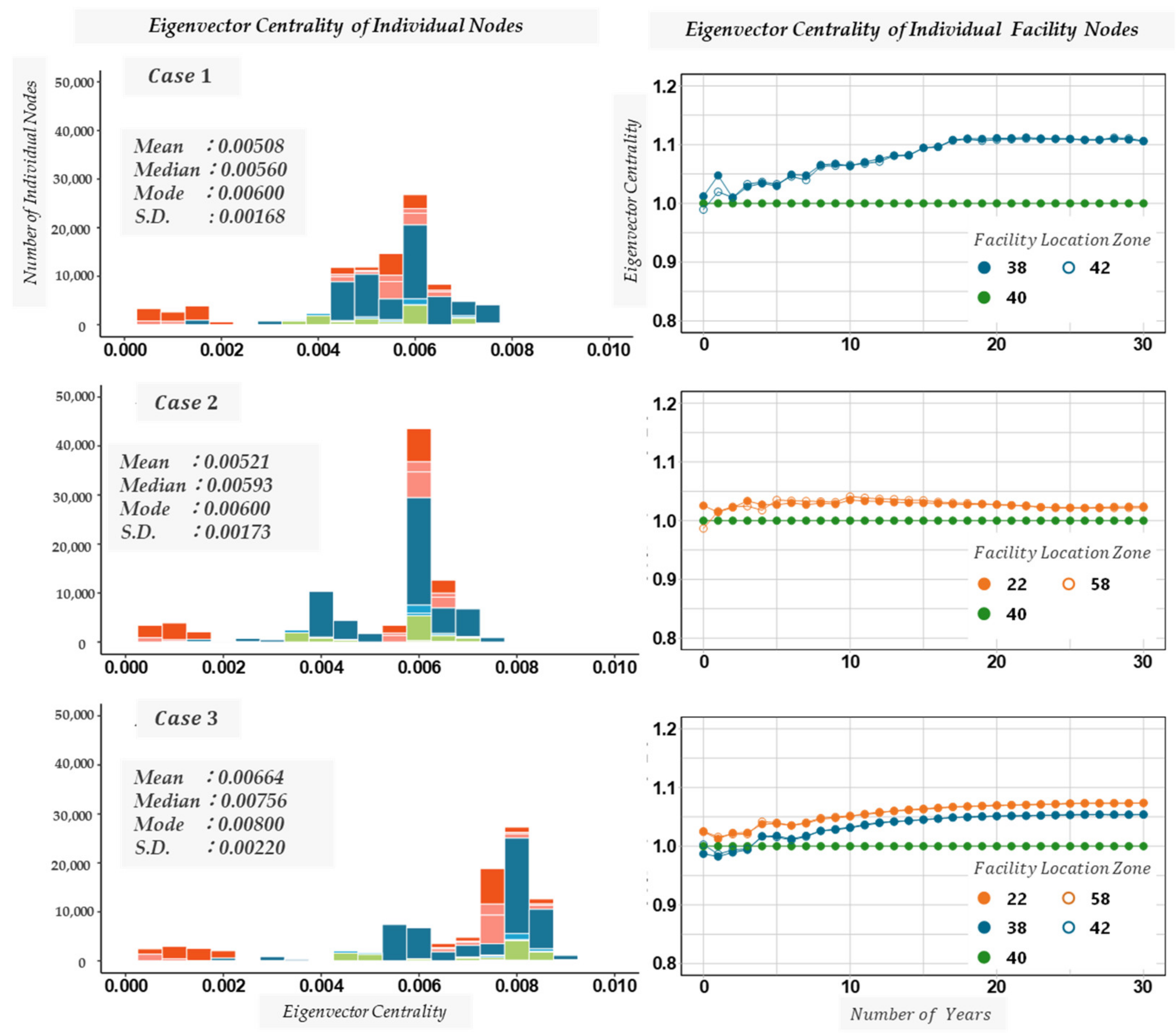
The results are interpreted focusing on the changes in the facility access network, mainly the EC of individuals and facility nodes. Figure 11 shows the distribution of EC of individual nodes and the temporal change of EC of facility nodes in the final year of the simulation (30th year). The distribution shape of EC of individual nodes in the final year can be considered as the distribution of individual accessibility under the condition that the household locations in the city are generally dynamically balanced.
Focusing on the distribution shape, it can be confirmed that the average value of EC is larger in case 3 compared to cases 1 and 2. Specifically, as the number of facilities in the city increases, the number of individuals also increases, and the eigenvector centrality is estimated to be averagely large. Therefore, it is believed that the EC of an individual with high accessibility will increase.
In addition, it can be seen that the EC of the facility node converges to a constant value in all cases in the latter half of the simulation in which the household location is dynamically balanced. Moreover, it can be confirmed that the difference in EC at that time is unique to each set case. To be precise, the EC of the facility corresponding to the household location according to the facility distribution in the city was calculated.
4. Discussion
4.1. Findings and Implications
The simulation results of population and number of households presented in Section 3.2 show the aging and prediction of smaller household sizes in real cities. In addition, the changes in traffic conditions, such as road congestion and public transportation facilities and services presented in Section 3.3, obtained appropriate results for the setting of the transportation network.
From these results, we confirmed that the simulation model is useful for expressing demographic changes and traffic conditions. In Section 3.4, we conducted an analysis using EC and confirmed that accessibility between facilities and households can be expressed as a network index to evaluate the dynamic changes of urban structure from the shape theory (topology) of the network perspective.
The method is based on simulations and several models, and each processing step is easy to carry out or understand. Our model expresses social dynamics by accumulating such simple individual changes and choice behaviors. In addition, it has high extensibility by improving individual submodels. On the contrary, extensive data requirements for calibration and excessively long computing times are significant issues to the implementation of microsimulations [2].
In urban planning, considering changes in land use is vital, and we considered land use by focusing on the distribution of households and population as land use. Additionally, we integrated the housing location choice model into our models to represent the future situation of the simulated city.
Subsequently, despite conducting 30 years of future simulations, this period is not designated for the simulation of 30 years more or less. Of course, a short-term forecast would be more reliable compared to the long-term forecast, which can be used for short-term planning, such as the supply of services and plan for operations.
However, a long-term future forecast is required for preparing long-term plans, such as the city’s conceptual plans, master plans, and development directions, which decide the future condition of a city and considerably contribute to the sustainability of the city. With such a long-term forecast, we can begin to plan for the next 20 or 30 years. Of course, after passing each period (year), we can again forecast or simulate to compare the actual changes and simulation results. Based on the actual changes, a resimulation will be done, and the plans will be updated.
The method of this study using a multi-layer network expresses the attributes of agents, such as individuals and households and their changes as dynamic changes in the network and its shape. The academic contribution of this study is to extend the existing microsimulation-based urban models to a network-based model by describing the interrelationship between an entity and a network in urban space, and as a result, a complex and large-scale urban structure can be expressed. In addition, a basic method for expressing and evaluating social dynamics was developed by evolving social network analysis, which has been statically analyzed, into network dynamics that include the shape changes.
It is necessary to improve the adaptability of models to social threats, such as rapid aging, depopulation, and frequent disasters, and to ensure the sustainability of society. On the other hand, society constantly changes its appearance due to various adaptive behaviors of decision-makers. In this study, we proposed a dynamic simulation method to capture such social change phenomena and to understand and describe the social states that can occur as a result of the adaptive behavior of the subject.
The significance of this research from the perspective of policymaking and evaluation is its applicability as a basic method for considering the effects of various policies to realize a sustainable urban design, such as land use regulation, residence guidance, urban service facility placement, and transportation network improvement. Furthermore, this work has the potential to consider the timing of the implementation of these policy measures.
4.2. Limitations
As we are in the first step of the introduction of this method, due to the model simplicity we did not represent certain attributes and factors in our models. In addition, since the household composition and its transition and life events, were modeled while considering the characteristics of Japan, some social dynamic characteristics that are common in other developed countries were not considered.
For instance, there are unmarried couples and cohabiting couples without any legal regulation, who are not registered especially in western countries. However, the rate of cohabiting couples in Japan is very low, accounting for less than 2% of singles, according to 2015 statistics from the National Institute of Population and Social Security Research (IPSS) [42].
Similarly, birth has been defined as a life event that occurs only in married women. In many countries, women give birth to a child regardless of their marital status. However, the birth rate of unmarried women in Japan is very low at 2.3% [43]. It is difficult to obtain sufficient statistical data for these to be considered in the model. Therefore, in this stage of model development, we considered only cohabiting couples with legal agreements and assigned births to married women.
Moreover, the purpose of this study is to show a newly developed method to simulate the future situation of a city by implementing the method in a virtual city. To make it more simplified and easier to understand, we did not include certain attributes. However, the attributes of a real city can be added to this model, and the model easily appreciates any introduction of new attribute classification. For instance, in the current version of the model, the expression of location choice characteristics (for instance, that young households with a low-purchasing power may move to the surrounding areas with low housing cost rates, and wealthy social classes may choose more luxurious and protected residential areas outside the city) have not been considered.
Nonetheless, we used the land price model and housing location choice model in our simulation. Therefore, the housing cost is considered indirectly by the elaboration of changes in the land price. With the integration of the housing market model, it is possible to analyze the resident’s more detailed location choice behavior, and our model has a basic structure that allows for such improvements.
These factors need to be considered in the model depending on the characteristics of the region to which they are applied and the objective of the policy analysis. Since we express social dynamics as a stack of simple life events and selective behaviors based on micro-simulation methods, our model has the potential to accept new relative factors and attributes and expand their expressions.
5. Conclusions
Japan, as with any other developed country, has its hurdles to reach and maintain sustainable cities. In this study, we developed a method that can be useful for the evaluation of different sustainable urban policies by focusing on social dynamics, land use, and transportation networks. We described the urban space with a network and modeled its dynamics to examine the possibility of urban analysis focusing on the network setting and evaluation by network indicators.
The simulation method is based on a microsimulation model consisting of several models, where each processing step is easy to carry out or understand. Our model expresses social dynamics by accumulating simple individual changes and choice behaviors. We analyzed individual facility access using eigenvector centrality, and the results were used for further interpretation of this research.
As a result, it was suggested that the individual’s eigenvector centrality could be an index of individual access to the facility. It was also suggested that the eigenvector centrality of the facility can be a quantitative index of the accessibility of the facility to individuals, considering both aspects of the facility location and the household location. Since these indicators fluctuate with the temporal change of facility location and household location distribution in urban space, it is suggested that they can be accessibility indicators that reflect the location of urban space.
In this study, we attempted to describe the urban space by using a layer-divided k-partite network. However, multilayer networks are classified into many types based on restrictions on the connection method within and between layers. As a further study, it is necessary to repeatedly study the shape and evaluation index based on the characteristics of each network expression.
Furthermore, the application of a model for a real city is indispensable for examining a practical analysis method. Therefore, we plan to carry out simulations targeting the population/household composition, land use, and transportation networks of an actual city to confirm their behavior and to examine their practicality and reproducibility as an analysis method.
Author Contributions
Conceptualization, N.S. and F.K.; methodology, N.S. and S.N.; software, K.M.; validation, N.S.; formal analysis, N.S. and S.N.; investigation, N.S., S.N. and M.M.; resources, N.S. and K.M.; data curation, S.N.; writing—original draft preparation, N.S. and S.N.; writing—review and editing, N.S. and M.M.; visualization, S.N. and M.M.; supervision, N.S.; funding acquisition, N.S. and F.K. All authors have read and agreed to the published version of the manuscript.
Funding
This research was funded by the Japan Society for the Promotion of Science (JSPS) under the Grant-in-Aid for Scientific Research (B) JP18H01557, and (C) JP20K04721.
Institutional Review Board Statement
Not applicable.
Informed Consent Statement
Not applicable.
Data Availability Statement
Publicly available datasets were analyzed in this study. These can be found here: National census, https://www.stat.go.jp/english/index.html; Vital statistics, https://www.mhlw.go.jp/english/database/db-hw/index.html; Basic school survey, https://www.mext.go.jp/en/publication/statistics/index.htm; Driver’s license statistics, https://www.npa.go.jp/publications/statistics/koutsuu/menkyo.html.
Conflicts of Interest
The authors declare no conflict of interest.
References
- Wegener, M. Overview of Land-Use Transport Model. In Proceedings of the CUPUM’03, Sendai, Japan, 27–29 May 2003. [Google Scholar]
- Wegener, M. Integrated land-use transport modelling progress around the globe. In Proceedings of the Fourth Oregon Symposium on Integrated Land-Use Transport Models, Portland, OR, USA, 15–17 November 2005. [Google Scholar]
- Waddell, P. UrbanSim: Modeling urban development for land use, transportation, and environmental planning. J. Am. Plan. Assoc. 2002, 68, 297–314. [Google Scholar] [CrossRef]
- Hunt, J.D.; Donnelly, R.; Abraham, J.E.; Batten, C.; Freedman, J.; Hicks, J.; Costinett, P.J.; Upton, W.J. Design of a statewide land use transport interaction model for Oregon. In Proceedings of the 9th World Conference on Transport Research, Seoul, Korea, 22–27 July 2001. [Google Scholar]
- Abraham, J.E.; Garry, G.R.; Hunt, J.D. The Sacramento Pecas model. In Proceedings of the Transportation Research Board Annual Meeting, Washington, DC, USA, 9–13 January 2005. [Google Scholar]
- Hunt, J.D.; Abraham, J.E. Pecas-for Spatial Economic Modelling: Theoretical Formulation; System Documentation Technical Memorandum 1 Working Draft; 2009. Available online: https://www.hbaspecto.com/resources/PECASTheoreticalFormulation.pdf (accessed on 2 December 2021).
- Salvini, P.; Miller, E.J. ILUTE: An operational prototype of a comprehensive microsimulation model of urban systems. Netw. Spat. Econ. 2005, 5, 217–234. [Google Scholar] [CrossRef]
- Moeckel, R.; Spiekermann, K.; Wegener, M. Creating a synthetic population. In Proceedings of the 8th International Conference on Computers in Urban Planning and Urban Management, Sendai, Japan, 27–29 May 2003. [Google Scholar]
- Strauch, D.; Moeckel, R.; Wegener, M.; Gräfe, J.; Mühlhans, H.; Rindsfüser, G.; Beckmann, K.J. Linking transport and land use planning: The microscopic dynamic simulation model ILUMASS. In Geodynamics; CRC Press: Boca Raton, FL, USA, 2005; pp. 295–311. [Google Scholar]
- Ettema, D.; de Jong, K.; Timmermans, H.; Bakema, A. PUMA: Multi-agent modelling of urban systems. In Modelling Land-Use Change; Springer: Berlin/Heidelberg, Germany, 2007; pp. 237–258. [Google Scholar]
- Chengxiang, Z.; Chunfu, S.; Jian, G.; Chunjiao, D.; Hui, Z. Agent-based joint model of residential location choice and real estate price for land use and transport model. Comput. Environ. Urban Syst. 2016, 57, 93–105. [Google Scholar]
- Newman, M.E.J. Networks; Oxford University Press: Oxford, UK, 2010. [Google Scholar]
- Wasserman, S.; Faust, K. Social Networks Analysis: Methods and Applications; Cambridge University Press: Cambridge, UK, 1994. [Google Scholar]
- Jamali, M.; Abolhassani, H. Different Aspects of Social Network Analysis. In Proceedings of the 2006 IEEE/WIC/ACM International Conference on Web Intelligence (WI 2006 Main Conference Proceedings) (WI’06), Hong Kong, China, 18–22 December 2006. [Google Scholar]
- Bavelas, A. A mathematical model for group structures. Appl. Anthropol. 1949, 7, 16–30. [Google Scholar] [CrossRef]
- Uchida, M.; Shirayama, S. Analysis of network structure and model estimation for SNS. J. Inf. Process. 2006, 47, 2840–2849. [Google Scholar]
- Tsugawa, S.; Ohsaki, H. Community structure and interaction locality in social networks. J. Inf. Process. 2015, 23, 402–410. [Google Scholar] [CrossRef] [Green Version]
- Mehmet, F.; Hakan, A.; Hakan, K.; Köksal, B. Determining open education related social media usage trends in Turkey using a holistic social network analysis. Educ. Sci. Theory Pract. 2017, 17, 1361–1382. [Google Scholar]
- Yie, K.-Y.; Chien, T.-W.; Yeh, Y.-T.; Chou, W.; Su, S.-B. Using Social Network Analysis to Identify Spatiotemporal Spread Patterns of COVID-19 around the World: Online Dashboard Development. Int. J. Environ. Res. Public Health 2021, 18, 2461. [Google Scholar] [CrossRef] [PubMed]
- Kim, E.-J.; Lim, J.-Y.; Kim, G.-M.; Kim, S.-K. Nursing Students’ Subjective Happiness: A Social Network Analysis. Int. J. Environ. Res. Public Health 2021, 18, 11612. [Google Scholar] [CrossRef] [PubMed]
- Camarasa, C.; Heiberger, R.; Hennes, L.; Jakob, M.; Ostermeyer, Y.; Rosado, L. Key Decision-Makers and Persuaders in the Selection of Energy-Efficient Technologies in EU Residential Buildings. Buildings 2020, 10, 70. [Google Scholar] [CrossRef] [Green Version]
- Maskil-Leitan, R.; Gurevich, U.; Reychav, I. BIM Management Measure for an Effective Green Building Project. Buildings 2020, 10, 147. [Google Scholar] [CrossRef]
- Senaratne, S.; Rodrigo, M.N.N.; Jin, X.; Perera, S. Current Trends and Future Directions in Knowledge Management in Construction Research Using Social Network Analysis. Buildings 2021, 11, 599. [Google Scholar] [CrossRef]
- Tamura, S.; Namerikawa, S.; Murakami, K.; Yamanaka, H.; Sawada, T.; Hanaoka, F. A study on monitoring method of the network between participatory process using by the social network analysis. Proc. Infrastruct. Plan. 2005, 32, 158_1–158_4. [Google Scholar]
- Gomyo, M. Study of remote islands networks by analogy with graph theory. J. Jpn. Soc. Civ. Eng. B3 2013, 69, I_604–I_609. [Google Scholar]
- Masuda, N.; Konno, N. Complex Network: From Basics to Applications; Kindai Kagaku Sha: Tokyo, Japan, 2010. [Google Scholar]
- Nakaminami, T.; Nakayama, S.; Kobayashi, S.; Yamaguchi, H. Vulnerability assessment of emergency transportation road networks based on eigenvalue analysis. J. Jpn. Soc. Civ. Eng. D3 2018, 74, I_1141–I_1148. [Google Scholar]
- Ando, H.; Kurauchi, F. Evaluation of road network investment by using network topology method. J. Jpn. Soc. Civ. Eng. D3 2020, 75, I_445–I_454. [Google Scholar] [CrossRef]
- Ando, H.; Michael, B.; Kurauchi, F.; Wong, K.I.; Cheung, K.F. Connectivity evaluation of large road network by capacity-weighted eigenvector centrality analysis. Transp. A Transp. Sci. 2021, 17, 648–674. [Google Scholar] [CrossRef]
- Kuwano, M. Study on the comparison of social network characteristics by population size. J. City Plan. Inst. Jpn. 2014, 49, 999–1004. [Google Scholar]
- Kuwano, M.; Fykuyama, K.; Inoue, W. A study on relationship between human ties and individuals’ security feeling based on social network analyseses. J. Jpn. Soc. Civ. Eng. D3 2016, 72, 415–422. [Google Scholar]
- Kuwano, M.; Fykuyama, K. An analysis of accessibility of life-related facilities considering social networks. J. Jpn. Soc. Civ. Eng. D3 2015, 71, 293–303. [Google Scholar]
- Guancen, W.; Jing, L.; Dan, C.; Xing, N. Analysis on the Housing Price Relationship Network of Large and Medium-Sized Cities in China Based on Gravity Model. Sustainability 2021, 13, 4071. [Google Scholar]
- He, S.; Mei, L.; Wang, L. The Dynamic Influence of High-Speed Rail on the Spatial Structure of Economic Networks and the Underlying Mechanisms in Northeastern China. Int. J. Geo-Inf. 2021, 10, 776. [Google Scholar] [CrossRef]
- Jiao, L.; Li, D.; Zhang, Y.; Zhu, Y.; Huo, X.; Wu, Y. Identification of the Key Influencing Factors of Urban Rail Transit Station Resilience against Disasters Caused by Rainstorms. Land 2021, 10, 1298. [Google Scholar] [CrossRef]
- Porta, S.; Crucitti, P.; Latora, V. Multiple centrality assessment in Parma: A network analysis of paths and open spaces. Urban Des. Int. 2008, 13, 41–50. [Google Scholar] [CrossRef] [Green Version]
- Kivelä, M.; Arenas, A.; Barthelemy, M.; Gleeson, J.P.; Moreno, Y.; Porter, M.A. Multilayer networks. J. Complex Netw. 2014, 2, 203–271. [Google Scholar] [CrossRef] [Green Version]
- Tanimoto, K.; Maki, S.; Kita, H. Accessibility measure for public transportation planning in rural areas. J. Jpn. Soc. Civ. Eng. D 2009, 65, 544–553. [Google Scholar] [CrossRef]
- Harata, N. Disaggregate Behavioral Model and Multidimensional Choice. Infrastruct. Plan. Rev. 1986, 4, 15–27. [Google Scholar] [CrossRef] [Green Version]
- Ben-Akiva, M.; Lerman, S.R. Discrete Choice Analysis; MIT Press: Cambridge, MA, USA, 1985. [Google Scholar]
- Sugiki, N.; Nagao, S.; Batzaya, M.; Suzuki, A.; Matsuo, K. Development of a household urban micro-simulation model (HUMS) using available open-data and urban policy evaluation. In Urban Informatics and Future Cities; The Urban Book Series; Springer: Berlin/Heidelberg, Germany, 2021; pp. 343–370. [Google Scholar]
- National Institute of Population and Social Security Research. The 15th Basic Survey on Birth Trends (National Survey on Marriage and Childbirth). Available online: https://www.ipss.go.jp/ps-doukou/j/doukou15/doukou15_gaiyo.asp (accessed on 2 December 2021).
- OECD Family Database. SF2.4: Share of Births Outside of Marriage. Available online: http://www.oecd.org/els/soc/SF_2_4_Share_births_outside_marriage.xlsx (accessed on 2 December 2021).
Figure 1.
Description of urban space with a multi-layer network.
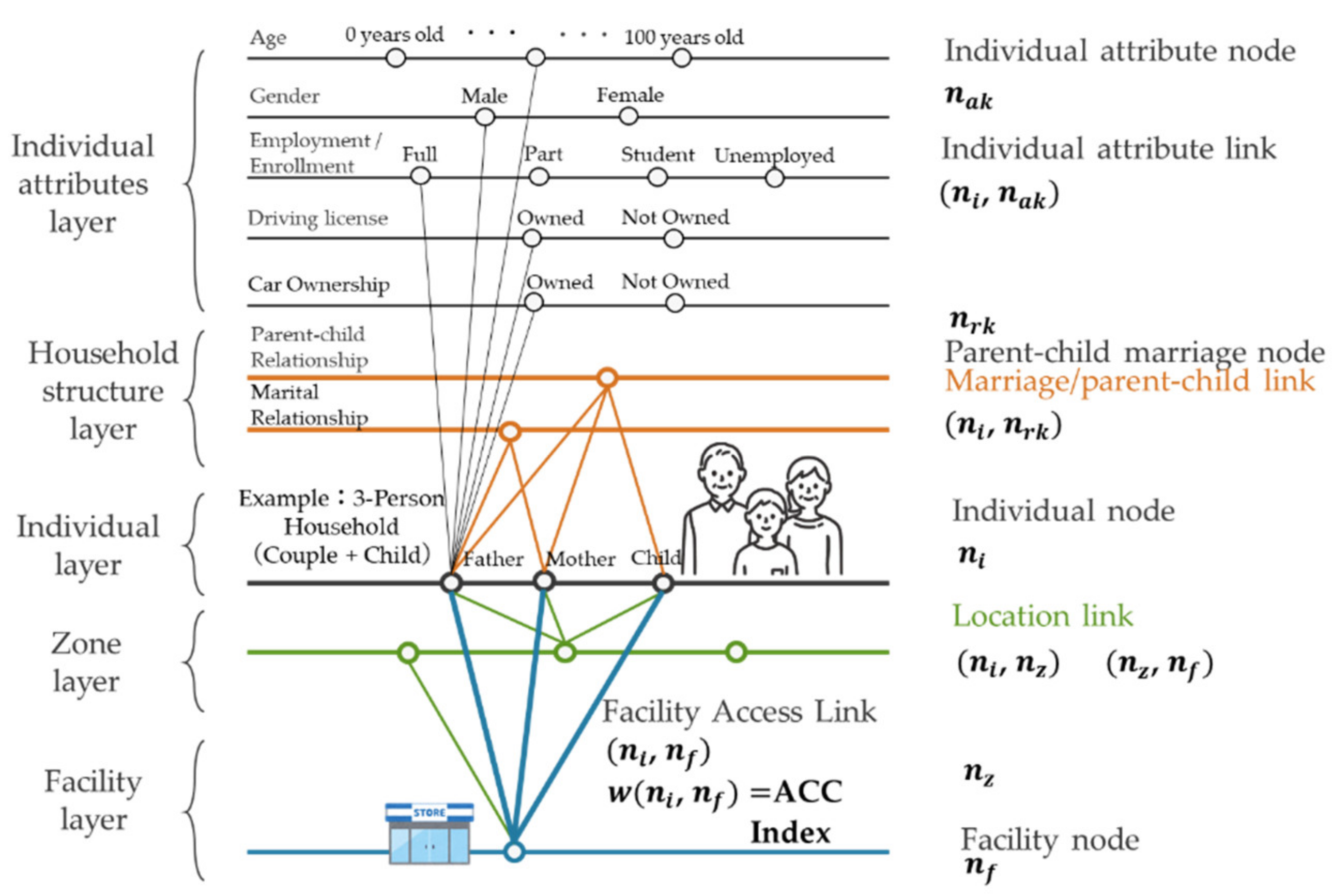
Figure 2.
The basic structure of the network dynamics.
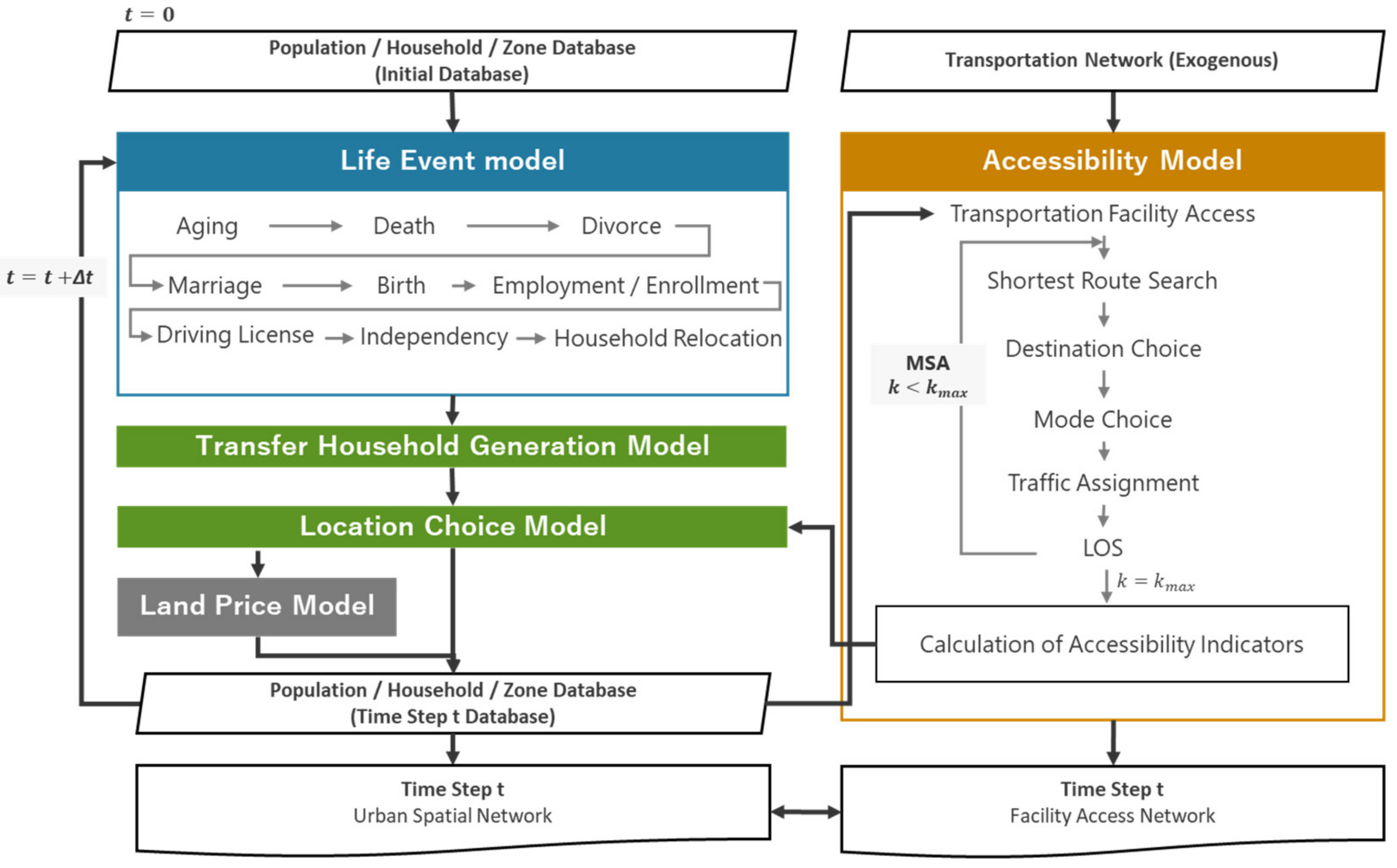
Figure 3.
Settings of the facility access network.
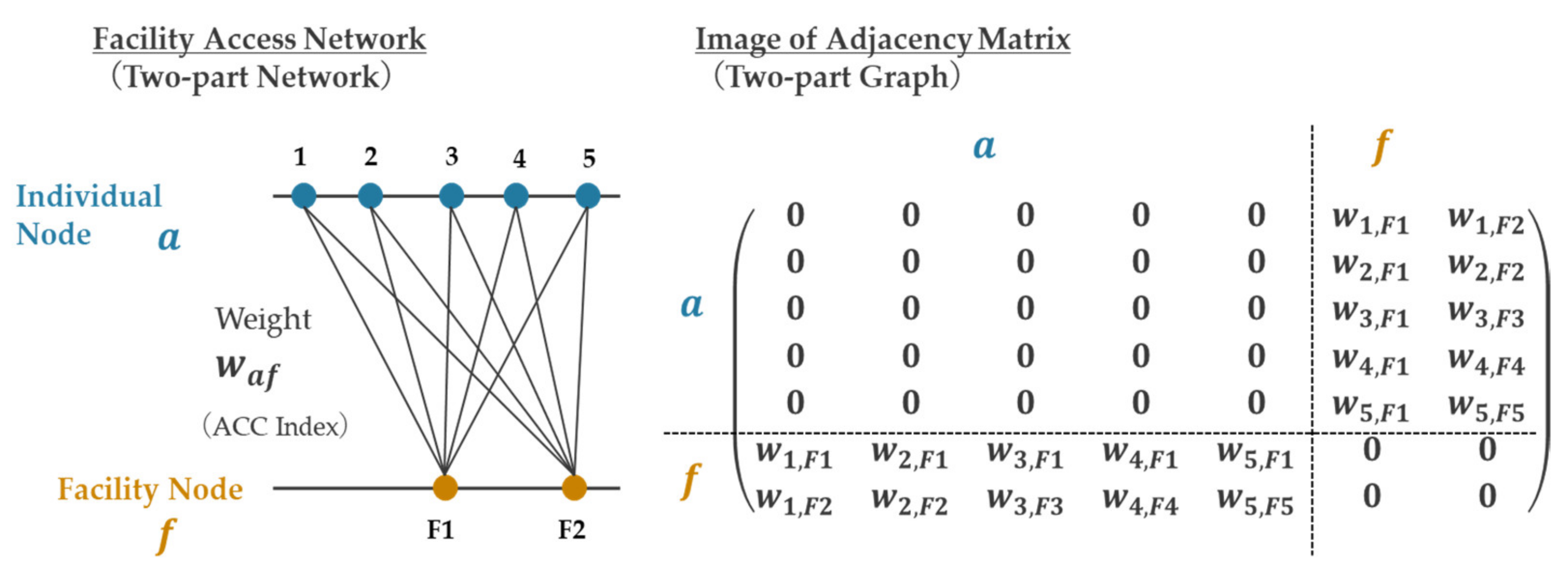
Figure 4.
Settings of the virtual city.

Figure 5.
Facility distribution in virtual cities. Case 1: Facility zone = 38, 40, and 42. Case 2: Facility zone = 22, 40, and 58. Case 3: Facility zone = 22, 38, 40, 42, and 58.
Figure 5.
Facility distribution in virtual cities. Case 1: Facility zone = 38, 40, and 42. Case 2: Facility zone = 22, 40, and 58. Case 3: Facility zone = 22, 38, 40, 42, and 58.

Figure 6.
Changes in the population and the number of households.
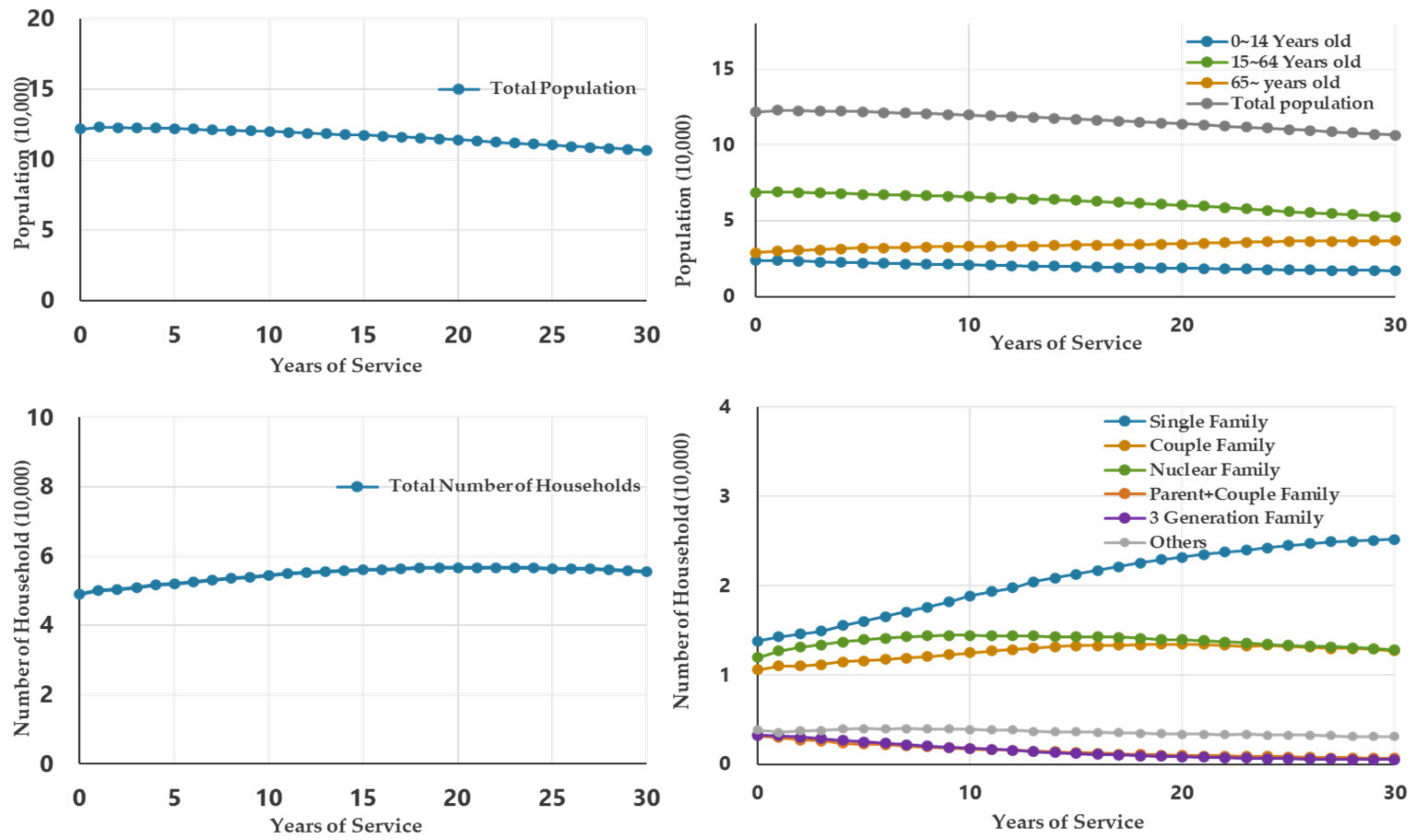
Figure 7.
Changes in population distribution by zone.

Figure 8.
Changes in the number of users by mode.
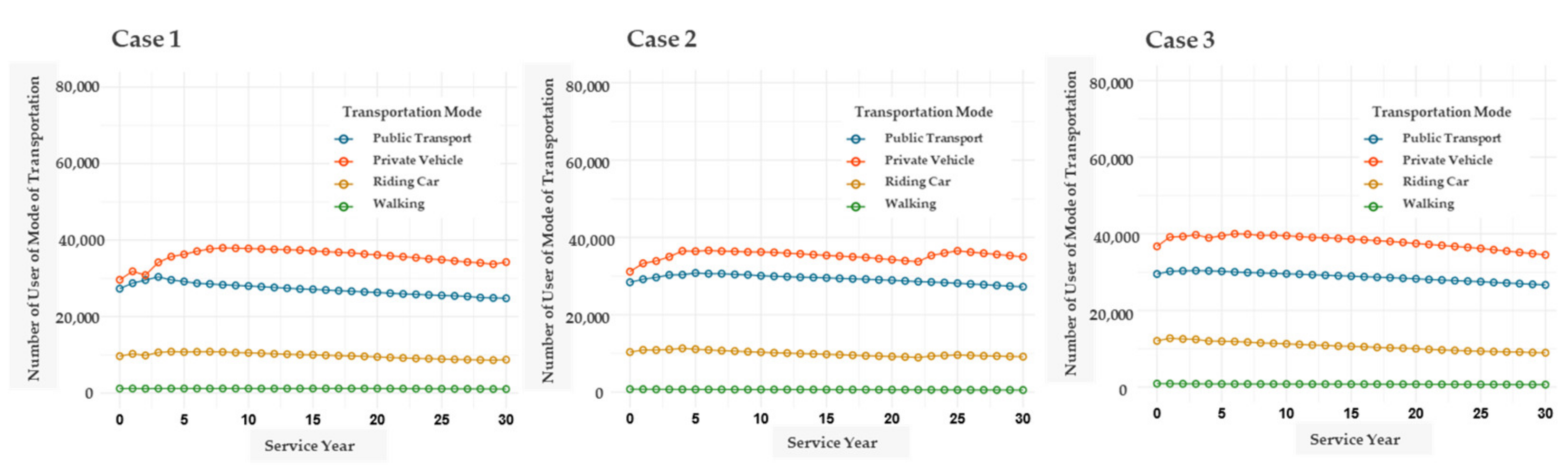
Figure 9.
Changes in the public transport frequency.

Figure 10.
Changes in the road congestion.

Figure 11.
Eigenvector centrality of facilities and individuals by case.

Table 1.
Factors for eigenvector centrality.
| Factors | Individual Node EC | Facility Node EC |
|---|---|---|
| Frequency | Number of Accessible Facilities | Number of Accessible Individuals |
| Weight | Individual Facility ACC Index | Individual Facility ACC Index |
| Adjacent Node EC | Facility Node EC Facility Accessibility | Individual Node EC Individual Accessibility |
Table 2.
Attributes and traffic conditions for each individual category.
| Individual Category n | Age | Availability of Transportation Mode | ||||||||
|---|---|---|---|---|---|---|---|---|---|---|
| Licensed | Driving | Public Transport | Walking | Riding | ||||||
 Elderly|Licensed Elderly|Licensed | 65– | 1 | 1 | 1 | 1 | 0 | ||||
 Non-Elderly|Licensed Non-Elderly|Licensed | 18–64 | 1 | 1 | 1 | 1 | 0 | ||||
 Elderly|No license (Shared) Elderly|No license (Shared) | 65– | 0 | 0 | 1 | 1 | 0.5 | ||||
 Elderly|No license (No Ride) Elderly|No license (No Ride) | 65– | 0 | 0 | 1 | 1 | 0 | ||||
 Non-Elderly|No license (Shared) Non-Elderly|No license (Shared) | 18–64 | 0 | 0 | 1 | 1 | 0.5 | ||||
 Non-Elderly|No license (No Ride) Non-Elderly|No license (No Ride) | 18–64 | 0 | 0 | 1 | 1 | 0 | ||||
 Child|No license (Shared) Child|No license (Shared) | 6–17 | 0 | 0 | 1 | 1 | 0.5 | ||||
 Child|No license (No Ride) Child|No license (No Ride) | 6–17 | 0 | 0 | 1 | 1 | 0 | ||||
| Individual Category n | Walking Speed | Walking Walkable Distance | Walking Time VoT | Waiting Time VoT | Ride Time VoT | Travel Cost Unit | Transfer Cost | Gen. Cost Parameter | Vehicle’s Constant Gen. Cost | |
| (km/h) | (km) | (Yen/Min) | (Yen/Min) | (Yen/Min) | (Yen/km) | (Yen/Times) | ||||
| Elderly|Licensed | 0 | 2.4 | 0.5 | 300 | 50 | 50 | 20.8 | 100 | −1 | 3000 |
| Non-Elderly|Licensed | 1 | 4.8 | 1.0 | 150 | 50 | 50 | 20.8 | 50 | −1 | 1500 |
| Elderly|Unlicensed (Shared) | 2 | 2.4 | 0.5 | 300 | 50 | 50 | 20.8 | 100 | −1 | 3000 |
| Elderly|Unlicensed (No Ride) | 3 | 2.4 | 0.5 | 300 | 50 | 50 | 20.8 | 100 | −1 | 3000 |
| Non-Elderly|Unlicensed (Shared) | 4 | 4.8 | 1.0 | 150 | 50 | 50 | 20.8 | 50 | −1 | 1500 |
| Non-Elderly|Unlicensed (No Ride) | 5 | 4.8 | 1.0 | 150 | 50 | 50 | 20.8 | 50 | −1 | 1500 |
| Child|Unlicensed (Shared) | 6 | 4.8 | 1.0 | 150 | 50 | 50 | 20.8 | 50 | −1 | 1500 |
| Child|Unlicensed (No Ride) | 7 | 4.8 | 1.0 | 150 | 50 | 50 | 20.8 | 50 | −1 | 1500 |
Table 3.
Traffic network conditions and model parameters.
| (a) Traffic Network Conditions | ||||||||||
|---|---|---|---|---|---|---|---|---|---|---|
| Transport Mode | System | Capacity | Seat Capacity | Minimum Frequency | Maximum Frequency | Terminal Charges | Distance Cost | |||
| l | (Person/Mode) | (Person/Mode) | (Mode/Time) | (Mode/Time) | (Yen/Times) | (Yen/km) | ||||
| Train | East-West (Left and Right) | 200 | 100 | 2 | 10 | 100 | 20 | |||
| Bus | North-South (Top and Bottom) | 200 | 100 | 2 | 10 | 100 | 30 | |||
| Bus | Circulated | 60 | 30 | 2 | 10 | 100 | 30 | |||
| (b) Residential Location Choice Model | (c) Land Price Model | |||||||||
| Variables | Parameter | Variables | Parameter | |||||||
| Land Price (10,000 Yen) | −0.1 | City Center (Central Mesh)Distance (km) *Common Logarithm | −8.0 | |||||||
| City Center (Zone Centroid)Distance (km) *Common Logarithm | −0.2 | Nearest Station Distance (km) *Common Logarithm | −4.0 | |||||||
| Nearest Station Distance (km) *Common Logarithm | −0.4 | Population density = Population/Zone Area (Person/ha) | 0.1 | |||||||
| Household Synthetic ACC | 0.5 | Constant | 20 | |||||||
| (d) Facility(Destination)Unit Indicator | (e) Generalized Cost Threshold | |||||||||
| Facility Zone | Unit Indicator | Facility Zone | Unit Indicator | Transportation | Threshold (Yen) | |||||
| 22 | 500 | 42 | 500 | Private Vehicle | 1000 | |||||
| 38 | 500 | 58 | 500 | Car Riding | 1000 | |||||
| 40 (Central Zone) | 1500 | Public Transport | 3300 | |||||||
Publisher’s Note: MDPI stays neutral with regard to jurisdictional claims in published maps and institutional affiliations. |
© 2021 by the authors. Licensee MDPI, Basel, Switzerland. This article is an open access article distributed under the terms and conditions of the Creative Commons Attribution (CC BY) license (https://creativecommons.org/licenses/by/4.0/).
Share and Cite
MDPI and ACS Style
Sugiki, N.; Nagao, S.; Kurauchi, F.; Mutahari, M.; Matsuo, K. Social Dynamics Simulation Using a Multi-Layer Network. Sustainability 2021, 13, 13744. https://doi.org/10.3390/su132413744
AMA Style
Sugiki N, Nagao S, Kurauchi F, Mutahari M, Matsuo K. Social Dynamics Simulation Using a Multi-Layer Network. Sustainability. 2021; 13(24):13744. https://doi.org/10.3390/su132413744
Chicago/Turabian StyleSugiki, Nao, Shogo Nagao, Fumitaka Kurauchi, Mustafa Mutahari, and Kojiro Matsuo. 2021. "Social Dynamics Simulation Using a Multi-Layer Network" Sustainability 13, no. 24: 13744. https://doi.org/10.3390/su132413744
Note that from the first issue of 2016, this journal uses article numbers instead of page numbers. See further details here.