
Minimizing the Utilized Area of PV Systems by Generating the Optimal Inter-Row Spacing Factor
by
 , , and
Ayman Al-Quraan
1,* ,
,
Mohammed Al-Mahmodi
2 ,
,
Khaled Alzaareer
3,
Claude El-Bayeh
4 and
and
Ursula Eicker
4 1
Electrical Power Engineering Department, Hijjawi Faculty for Engineering Technology, Yarmouk University, Irbid 21163, Jordan
2
Mechanical Engineering Department, Renewable Energy, The University of Jordan, Amman 11942, Jordan
3
Department of Electrical Engineering, Faculty of engineering, Philadelphia University, Amman 19392, Jordan
4
Canada Excellent Research Chair Team, Concordia University, Montreal, QC H3H 2L9, Canada
*
Author to whom correspondence should be addressed.
Sustainability 2022, 14(10), 6077; https://doi.org/10.3390/su14106077
Submission received: 27 February 2022
/
Revised: 10 May 2022
/
Accepted: 11 May 2022
/
Published: 17 May 2022
(This article belongs to the Special Issue Sustainability of Smart Energy Grids: Pathway for Achieving a Green Smart Energy Grid)
Abstract
:In mounted photovoltaic (PV) facilities, energy output losses due to inter-row shading are unavoidable. In order to limit the shadow cast by one module row on another, sufficient inter-row space must be planned. However, it is not uncommon to see PV plants with such close row spacing that energy losses occur owing to row-to-row shading effects. Low module prices and high ground costs lead to such configurations, so the maximum energy output per available surface area is prioritized over optimum energy production per peak power. For any applications where the plant power output needs to be calculated, an exact analysis of the influence of inter-row shading on power generation is required. In this paper, an effective methodology is proposed and discussed in detail, ultimately, to enable PV system designers to identify the optimal inter-row spacing between arrays by generating a multiplier factor. The spacing multiplier factor is mathematically formulated and is generated to be a general formula for any geographical location including flat and non-flat terrains. The developed model is implemented using two case studies with two different terrains, to provide a wider context. The first one is in the Kingdome of Saudi Arabia (KSA) provinces, giving a flat terrain case study; the inter-row spacing multiplier factor is estimated for the direct use of a systems designer. The second one is the water pump for agricultural watering using renewable energy sources, giving a non-flat terrain case study in Dhamar, Al-Hada, Yemen. In this case study, the optimal inter-row spacing factor is estimated for limited-area applications. Therefore, the effective area using the proposed formula is minimized so that the shading of PV arrays on each other is avoided, with a simple design using the spacing factor methodology.
1. Introduction
The penetration level of small-scale renewable energy resources, particularly photovoltaic (PV) systems, has rapidly evolved over recent years. Their low installation and operational costs make these resources competitive in the energy market in those countries that have high solar radiation, such as those located in the Middle East and South Africa (MENA). Several studies have been conducted to investigate the possibilities of maximizing the yield of energy production from renewable power generation, taking the MENA region as a case study, using intensive surveys and theories of theoretical and practical optimization [1,2,3]. With more focus on PV systems, roof-top solar energy projects are incentivized due to the simplicity of grid integration and the possibility of trade and exchange within the grid via certain policies [4]. Furthermore, prompt implementation with scalable capacity and a low maintenance cost encouraged communities, households, and companies to invest in PV systems. One of the main hurdles encountered by systems designers is accommodating the area with the targeted demand without affecting the quantity and quality of the yielded energy.
Several studies have analyzed solar energy system designs from a variety of perspectives. For instance, many studies are devoted to studying the grid integration of solar energy systems and its impact on system quality, sustainability, and reliability [5,6,7]. Others concentrate on solar radiation assessments for different locations on Earth [8,9]. A concrete design for a solar energy system was also introduced in several studies, discussing the sizing, tracking system, maximum power point tracking (MPPT), and the power electronic devices. Nevertheless, there is a deficiency in the article’s content when it comes to effective area maximization in PV systems design. The studies that introduced the surface area are limited to the available area, suitable tilt angles, etc.
The sun’s path differs from one season to another, as well as varying based on the location around the globe. The winter season is the time when the elevation angle of the sun is at its minimum, which is the case when shading is at its maximum [10]. The variation in sun position is addressed by the researcher by studying the optimal orientation of PV panels to maximize as much extracted energy as possible. Karafil et al. [11] carried out a mathematical analysis and calculated the optimal tilt angle of the system, comparing the result with the practical data acquired. The shading effect is analyzed in [12] using hill-shade analysis, considering different levels of the roof potential of a PV system: the physical, geographical, and technical aspects. Furthermore, a tracking system is undergoing development to follow the sun’s path and has consequently increased the system yield, as introduced in [13,14,15].
The system’s overall area is affected by two main factors, which are module dimension and inter-row spacing. The spacing between arrays depends on how much the module is tilted, i.e., the tilt angle of the PV panel. In one study [16], different inter-row spacing is simulated and compared to analyze the solar shading levels throughout the year. The effect of inter-row spacing on energy yield was also investigated in another study [17] using data analysis of the measurements of the energy production of large PV plants for the calculation of shading effects. Joshi et al. [18] investigate different spacing ratios relative to the module height and simulate each one using PVsyst software to identify the most adequate spacing. The authors of [19] provide a sensor design to detect the shading on the inter-row spacing, to enable the system designer to test the shading of the PV modules.
Different configurations are considered in PV systems design. These configurations manipulate the installation angles through certain orientations upon tilt and azimuth angles, as well as change the panel’s orientation from portrait to landscape and vice versa [20,21]. The performance of PV systems is mainly affected by the shading phenomenon. Some software has been developed to estimate the spacing between PV arrays. Others have been developed to facilitate PV system design in terms of sizing and energy calculations. For example, PVsyst and PVsol both provide sizing features and performance analysis [22,23,24]. Some features are designed to calculate panel distribution in the studied area, such as the Skelion feature in the SketchUp software [25]. The accuracy of all the software types varies between 5.00 and 18.75% in terms of percentage error, according to the results reported in [26,27]. The software that is most commonly used in estimating the spacing between arrays has limited accuracy and could not deal with the different configurations of panel distribution for either flat or non-flat terrains.
To the best of the authors’ knowledge, studies that have introduced this issue are almost completely confined to the articles listed in this manuscript, with certain weaknesses and gaps. For example, although the authors of [28] extensively examined commercial buildings and shading within the roof restrictions, they have not come up with a clear methodology or presented any mathematical model to justify the selected spacing areas; even the parameters used are vague. The same issue is found in another study [22], where inter-row spacing was selected without considering the worst-case scenario when shading is at the maximum, especially in the case study in Germany, which has a very small elevation angle that was ignored. Other studies tended to assume different spacing patterns and different orientations to investigate the impact of each selected value, as presented by the authors of [17,18]. The rest of the articles either relied on software directly or ignored some parameters, which is the case in [29,30,31]. Moreover, scholars have not paid significant attention to PV systems in the case of hilly sites and terrain restrictions. The research gap is that insufficient articles are available to clearly address the issue of shading by providing a clear and detailed methodology for the researcher and designer to select adequate inter-row spacing, considering the essential parameters and different configurations to ensure minimizing the shading area and maximizing the energy production.
Therefore, the contribution of this manuscript can be summarized as the following:
- Generating the optimal inter-row spacing factor for minimizing the installation area and maximizing the energy output of the PV system for flat and non-flat terrains.
- A detailed method of estimating the needed angles of the sun’s path, which play an essential role in systems design.
- A comprehensive description of inter-row spacing estimation is given to establish the most appropriate spacing that avoids the worst-case scenario of the shading effect.
- Generating an inter-row spacing factor formula and validating it through a case study that was conducted in the Kingdom of Saudi Arabia (KSA), which has high solar radiation and solar energy potential but insufficient studies in this regard.
The rest of this article is organized as follows: the methodology of sun angle calculation and factor generation is presented in Section 2. In Section 3, the methodology of optimum area estimation is introduced, while the objective function is presented in Section 4. Case studies and the validation process are introduced in Section 5, and Section 6 presents our conclusions.
2. Definitions and Methodology
2.1. Sun Angles Calculation
It is essential to identify the sun’s path at the system’s final location to understand the nature of shading over the course of a year, especially in the worst-case scenario when the objects’ shading is at maximum in the northern hemisphere on 21 December every year [27,32]. The first stage of designing a PV system sun chart is to consider and identify the required sun radiation angles; elevation and azimuth. Figure 1 illustrates an example of a two-dimensional (2D) sun path, and how these angles can be estimated by analyzing this chart. As shown at 9.00 a.m. and 3.00 p.m., the shading is the longest, so the figure represents the method of identifying the angles. It can be noticed from Figure 1 that on 21 December, the date when shading is at the maximum, the sun elevation angle is 28° and the azimuth angle is about 45°.
The elevation angle in the winter season is the smallest value, based on the rule that the smaller the elevation angle, the greater the shading of objects [34]. In the case of PV system installation, this angle is considered to avoid exposing the PV array to the shading of the array behind. To this end, intensive calculation is required to determine the optimal inter-row spacing between arrays. In this section, the methodology of selecting the most efficient space that ensures minimizing the area occupied and maximizing the energy production is introduced.
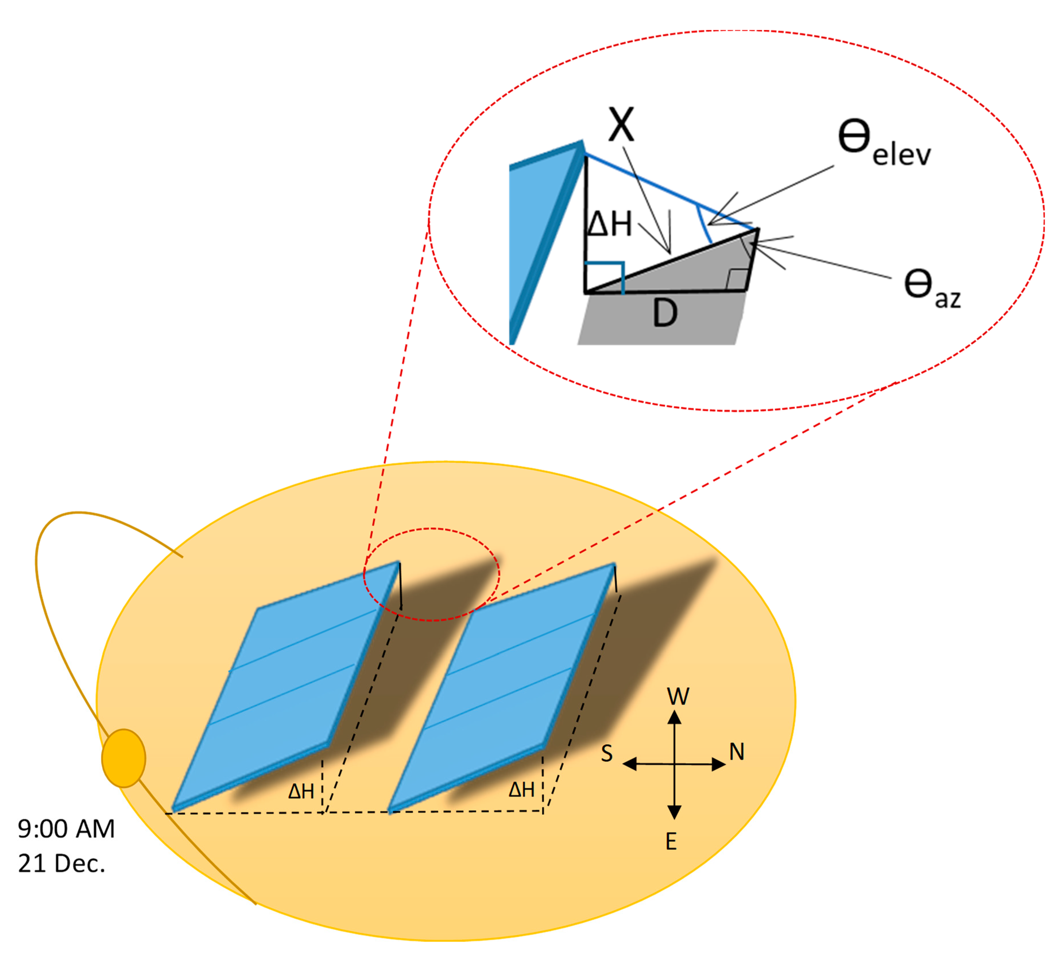
Different parameters are required to identify the distance between two rows. The first parameter is from the module dimension and whether the module is implemented individually or mounted in two modules. Then, the tilt angle that is selected by the designer is also required. In this step, the height difference, , which is shown in Figure 2, is estimated, assuming that the module shading has an angle with the horizontal called the azimuth angle, . As the elevation angle is determined from the sun’s path and the height difference is estimated from the module dimension and tilt angle, the shading length can consequently be determined and denoted by X. However, the shading has appeared with a length of X; this cannot be considered as the spacing value because it is tilted at an angle. The spacing, which is denoted by D, can be estimated using the X-value and the azimuth angle in the triangle when laid horizontally.
The inter-row spacing between PV arrays can be calculated by estimating these angles in addition to the dimensions of the panel used. Once these angles are graphically estimated, the inter-row spacing can be determined using the following formula:
where is the height of the module terminal, L is the PV panel length, and is the tilt angle of the module. Then, the inter-row spacing can be estimated using the following equation:
where X is the shadow length and is the sun elevation angle at the location, which can be determined from the sun’s path.
Figure 3 represents the two-dimensional geometry of solar panel implementation relative to the sun’s path, with inter-row spacing as D, height difference, and installation angles: tilt angle and elevation angle [35]. As shown in this figure, the elevation angle significantly affects the self-shading. This angle varies, based on the geographic location. The second parameter is the tilt angle, which depends on the system designer’s decision and may differ to accommodate a certain number of panels. Other parameters, D, L, and refer to the spacing between successive panels or arrays, the length of the module, and the height difference in the vertical projection of the module, respectively.
2.2. Multiplier Factor Estimation
In this paper, the optimal inter-row spacing factor is generated for a different location in Saudi Arabia to facilitate determining the optimum spacing between modules. By implementing this optimum spacing, shading will be minimized, and the utilized area will also be minimized. The designer can use this multiplier factor directly without going through complicated calculations. The factor can be estimated from the proposed formula, which is based on the sun elevation and azimuth angles:
where is the azimuth angle and is the elevation angle. This factor can be used by multiplying it with the height of the module :
Moreover, in cases where a limited area is available, the configuration of solar arrays might be oriented relative to the azimuth angle, with a certain angle to accommodate the available area. The inter-row spacing factor will remain the same and is not affected by orienting the panel from the optimal position, based on the new azimuth angle. Figure 4 shows that the whole triangle is rotating, keeping the distance, D, unchanged, like the radius of a circle. Thus, the inter-row spacing factor is still applicable.
2.3. Inter-Row Spacing Considered for Non-Flat Terrain
Hilly sites are always an option for installing PV systems with relative ease, but the land surface is not always flat. There may be terrain issues or roughness that should be taken into consideration in the shading analysis. The effect of these terrain issues might increase or decrease the shading phenomenon. Figure 5 illustrates a scenario using a PV system area with non-flat terrain, where the PV station is installed on uneven ground and is ascending or descending at a certain slope. In this case, arrays are installed either higher or lower than the previous array, corresponding to the south direction. As shown in this figure, array (2) is higher than array (1), which results in decreasing the shading; in contrast, array (5) is lower than array (4), which requires increasing the distance between them to avoid shading.
To properly address this issue, the first step is to identify the reference line between every two successive arrays, which is the horizontal line that passes through the lowest point. The idea behind drawing a reference line is to calculate the height difference between two or more bases of the PV arrays. Once the height difference (h) is estimated, the second step is to identify whether the slope is positive or negative. The inter-row spacing between two arrays in an area with a specific terrain will, therefore, be affected by the height difference. Therefore, the new formulation can be written to consider this new factor as follows:
If the slope is positive, as in slope 1, the height difference h1 will be positive (h); if the slope is negative, as in slope 2, the height difference h2 is negative (–h).
3. Methodology of Optimum Area Estimation
The PV system’s area is affected by different factors, which are the dimension of the module, the tilt angle, and the location on the Earth. The area’s location affects the length of the shading and the inter-row spacing accordingly. To minimize the area required for system installation, the optimal inter-row spacing needs to be estimated, taking into account maximizing the energy yield by selecting the optimal tilt angle of the system location. The area estimated is at optimum when shading is completely avoided; therefore, the area is properly utilized. Figure 6 illustrates the essential factors that are used to estimate the area, assuming certain dimensions of the PV panel and the spacing between arrays.
If the installed system encompasses the (n) number of vertical modules that have dimensions L × w, per (m) arrays, tilted at a tilt angle of , the spacing between rows is estimated and is equal to D. Thus, in the case of uniformly distributed modules, the whole system’s occupied area is equal to:
4. Objective Function
In the non-flat sites, the total area will be changed according to the terrain’s nature (see Figure 7). Thus, to estimate the overall area, the sum of the different areas needs to be determined, as follows:
where R and C are the rows and columns of the PV systems, respectively. In Equation (8), the areas between two successive modules in the system are estimated, where each area is affected by several parameters, taking into account the dimension of the PV panel, the inter-row spacing, and the terrain nature. Since there is no self-shading for the first row of the PV system, the inter-row spacing is not taken into account and the second part of Equation (8) is applied.
The general formula of the energy produced by the PV system (E) depends on several parameters, as suggested by the authors of [27]:
where AS is the surface area of the PV panel, r is the solar panel efficiency, GR is the tilted surface mean solar radiation, and PR is the performance ratio. Knowing this, the energy density is the ratio between the generated energy and the installation area:
where Ed is the energy density in (kWh/m2), Eout is the energy output in (kWh), and A is the total area of the system in (m2). If we substitute Equation (8) into Equation (10), then Ed can be written as follows:
The objective function in this study is to maximize the energy density by avoiding the shading effect, based on several constraints, as follows:
Objective function:
Subject to:
where Dworst is the inter-row spacing under the worst-case scenario (21 December).
5. Case Studies and Validation Process
5.1. Saudi Arabia Case Study
A case study has been developed to evaluate the multiplier factor for all provinces in KSA. Table 1 summarizes some general information about these provinces. In addition, the optimum multiplier factors for all provinces are also presented in this table. To validate the above methodology, a real-life installed system in Saudi Arabia, in Jeddah province, is tested under different scenarios by varying the tilt angle of the system arrays. This system is installed using a 15° tilt angle in reality. The number of the modules that are studied here is 750, distributed over five roof-tops, as shown in Figure 8. This system will be tested in two scenarios: uniformly distributed modules when the tilt angle is standardized throughout all the arrays, and non-uniformly distributed arrays, when more than one tilt angle is used for system area minimization. In the case of a standardized tilt angle, the above formula is used to calculate the overall system area.
In this case study, two different scenarios are presented to evaluate the methodology of minimizing the installation area of the PV system. The first scenario is to use the same tilt angle for all arrays, while the second scenario is to implement two tilt angles in the same system, as discussed in a previous study [27]. The area is divided into five areas, and the estimation in the first scenario is summarized in Table 2; the module length is 2L because every two modules are mounted together in the installed system. It is found that the area is reduced by 300 m2 due to the proposed approach of estimating the area, based on optimal inter-row spacing using the generated multiplier factor.
The second scenario is to implement the system by setting different tilt angles, as proposed by the authors of [27], setting the tilt angle of the first row to the optimal tilt angle, which is 22° in the studied case. This row now has a shadow effect on the other arrays because it is the first one to the north of the area of the rooftop. The optimal area, if this methodology is employed, is summarized in Table 3; the area is reduced by about 122 less than the standardized case, and, inevitably, the energy yield is maximized when setting the tilt angle of row 1 to 22°, the optimal angle.
In each scenario, a comparison between two different configurations is presented. The first configuration is designed to standardize a single tilt angle for all arrays in the system, while the second configuration is for the scenario of using two different tilt angles, according to the new configuration proposed by the authors of [27]. The optimal area that should be used is estimated and compared with the area that the system occupies in reality. The optimal area is calculated using the methodology proposed in this study, while the installation area is set based on a design tool that relied on the areas suggested by the software. The overall percentage error in the first configuration is 11.6%, and the percentage error, if the second configuration is employed, is 12.3%.
5.2. Yemen Case Study
Another case study in Yemen has been employed to extend the use of this mathematical model and provide a wider context for this study. The PV system in this study was installed in Dhamar, Al-Hada; longitude: 44.41423° and latitude: 14.5523°. It was designed by the Engineering Studies and Designs Unit–Tesla and was installed by Power City for electrical tools and solar energy systems, under the project name: “Water pump for agricultural watering, using renewable energy sources with a total power capacity of 52 kW”. A photo for this project is shown in Figure 9. As illustrated in this figure, the system is installed in a non-flat area in a descending order, facing the south direction. From inspection, the shading, in this case, will increase as we descend from array A1 to A4. The shading length of the PV arrays of this case study is also clearly shown in Figure 8.
The designer of this project selected the spacing between the PV arrays to prevent shading by ignoring the effect of the slope and the non-flat terrain. The actual total area of the spacing of the installed PV system is 370 m2, as illustrated in Table 4. However, since this value is sufficient to prevent shading in this case study, it cannot be employed in limited-area applications. Therefore, the mathematical model developed in this paper is used to provide the optimal inter-row spacing factor for limited area applications.
To estimate the optimal inter-row spacing factor between PV arrays, in this case, Equation (6) has been used with a positive height difference (h). Table 2 provides all the parameters needed to estimate the optimal inter-row spacing factor using this model. The estimated minimum spacing area that is sufficient to install this system with the same power capacity, ensuring avoidance of the worst-case scenario of the shading effect is 310.17 m2. As shown in Table 2, there are two different inter-row spacing distances between arrays in this case study. The first one is the inter-row spacing between the distant arrays A1 and A2, and A2 and A3. The second inter-row spacing is between A3 and A4. The former is less than the latter because its height difference is less than the latter, being 20 cm for the former, vs. 30 cm for the latter, as illustrated in Table 5. The optimal inter-row spacing factor is estimated for this case study, using Equation (4). Then, the spacing is decided, considering the non-flat terrain, using Equation (6). Considering these differences in terrain, the minimum spacing area is calculated using Equation (8) and is found to be less than the actual spacing area by around 16%.
6. Conclusions
As solar energy systems are rapidly proliferating in recent decades, and the potential dependency on this form of energy resource is increased, PV system installation and enhancement are being given significant attention by researchers worldwide. This article introduces a mathematical analysis of shading avoidance by the use of adequate spacing that ensures maximizing the extracted energy and minimizing the area occupied by the PV module. A complete formulation of the spacing factor has been developed and presented for flat and non-flat terrains. This factor can be generated and generalized to a specific geographical location, which could be a city or province.
In KSA, two specific scenarios were implemented for a flat-terrain PV system. A comparison of two distinct configurations was offered in each scenario. The first configuration applied a single tilt angle to all arrays in the system, while the second configuration employed two separate tilt angles to reduce the required area for PV system installation. The optimal area was determined using the approach given in this study, while the installation area was determined using the design software tool. Overall, the first setup had a percentage error of 11.6%, whereas the second configuration had a percentage error of 12.3%. To provide a broader perspective of this model, it was exemplified using a second case study with a non-flat terrain. This study is a water pump for agricultural watering using Renewable Energy sources located in Dhamar, Al-Hada, Yemen, which has a non-flat terrain. The optimal inter-row spacing factor for limited-area applications is estimated in this case study. The optimal spacing is reduced by around 16% from the actual spacing applied by the systems designers.
Author Contributions
Formal analysis, A.A.-Q. and M.A.-M.; Funding acquisition, A.A.-Q., K.A., C.E.-B. and U.E.; Investigation, A.A.-Q. and M.A.-M.; Methodology, A.A.-Q. and M.A.-M.; Project administration, A.A.-Q.; Software, M.A.-M.; Supervision, A.A.-Q.; Visualization, K.A., C.E.-B. and U.E.; Writing—original draft, M.A.-M.; Writing—review & editing, A.A.-Q. All authors have read and agreed to the published version of the manuscript.
Funding
This research received no external funding.
Institutional Review Board Statement
Not applicable.
Informed Consent Statement
Not applicable.
Acknowledgments
The authors acknowledge the Clean Environment Company, especially Engineer Taha Alasemi. They also acknowledge the Engineers from “Tesla for trading and engineering services”, Engineer Yahya Alhammadi, and Engineer Mohammed Habeb, for implementing the Yemen project and providing the required information and data. Yarmouk University and the University of Jordan are also acknowledged for their support in this study.
Conflicts of Interest
The authors declare no conflict of interest.
Abbreviations
| PV | photovoltaic |
| MENA | Middle East and South Africa (MENA) |
| MPPT | maximum power point tracking |
| 2-D | 2-dimensional |
| ΔH | PV panel height from the ground |
| θaz | Azimuth angle |
| θelev | Elevation angle |
| θtilt | Tilt angle |
| X | Shading length |
| D | Spacing between rows |
| L | PV panel length |
| w | PV panel width |
| F | Inter row spacing factor |
| h1 | Height difference with positive slope |
| h2 | Height difference with negative slope |
| A | PV system area |
References
- Al-Quraan, A.; Al-Qaisi, M. Modelling, Design and Control of a Standalone Hybrid PV-Wind Micro-Grid System. Energies 2021, 14, 4849. [Google Scholar] [CrossRef]
- Belaïd, F.; Elsayed, A.H.; Omri, A. Key drivers of renewable energy deployment in the MENA Region: Empirical evidence using panel quantile regression. Struct. Chang. Econ. Dyn. 2021, 57, 225–238. [Google Scholar] [CrossRef]
- Al-Quraan, A.; Al-Masri, H.; Al-Mahmodi, M.; Radaideh, A. Power curve modelling of wind turbines—A comparison study. IET Renew. Power Gener. 2022, 16, 362–374. [Google Scholar] [CrossRef]
- Al-Quraan, A.; Al-Mahmodi, M.; Radaideh, A.; AL-Masri, H. Comparative study between measured and estimated wind energy yield. Turk. J. Electr. Eng. Comput. Sci. 2020, 28, 2926–2939. [Google Scholar] [CrossRef]
- Panigrahi, R.; Mishra, S.K.; Srivastava, S.C.; Srivastava, A.K.; Schulz, N.N. Grid integration of small-scale photovoltaic systems in secondary distribution network—A review. IEEE Trans. Ind. Appl. 2020, 56, 3178–3195. [Google Scholar] [CrossRef]
- Tavakoli, A.; Saha, S.; Arif, M.T.; Haque, M.E.; Mendis, N.; Oo, A.M. Impacts of grid integration of solar PV and electric vehicle on grid stability, power quality and energy economics: A review. IET Energy Syst. Integr. 2020, 2, 243–260. [Google Scholar] [CrossRef]
- Al-Shetwi, A.Q.; Hannan, M.A.; Jern, K.P.; Alkahtani, A.A.; PGAbas, A.E. Power quality assessment of grid-connected PV system in compliance with the recent integration requirements. Electronics 2020, 9, 366. [Google Scholar] [CrossRef] [Green Version]
- Cornejo-Bueno, L.; Casanova-Mateo, C.; Sanz-Justo, J.; Salcedo-Sanz, S. Machine learning regressors for solar radiation estimation from satellite data. Sol. Energy 2019, 183, 768–775. [Google Scholar] [CrossRef]
- Babar, B.; Graversen, R.; Boström, T. Solar radiation estimation at high latitudes: Assessment of the CMSAF databases, ASR and ERA5. Sol. Energy 2019, 182, 397–411. [Google Scholar] [CrossRef]
- Awasthi, A.; Shukla, A.K.; SR, M.M.; Dondariya, C.; Shukla, K.N.; Porwal, D.; Richhariya, G. Review on sun tracking technology in solar PV system. Energy Rep. 2020, 6, 392–405. [Google Scholar] [CrossRef]
- Karafil, A.; Ozbay, H.; Kesler, M.; Parmaksiz, H. Calculation of optimum fixed tilt angle of PV panels depending on solar angles and comparison of the results with experimental study conducted in summer in Bilecik, Turkey. In Proceedings of the 2015 9th International Conference on Electrical and Electronics Engineering (ELECO), Bursa, Turkey, 26–28 November 2015; pp. 971–976. [Google Scholar]
- Hong, T.; Lee, M.; Koo, C.; Jeong, K.; Kim, J. Development of a method for estimating the rooftop solar photovoltaic (PV) potential by analyzing the available rooftop area using Hillshade analysis. Appl. Energy 2017, 194, 320–332. [Google Scholar] [CrossRef]
- Zhan, T.S.; Lin, W.M.; Tsai, M.H.; Wang, G.S. Design and implementation of the dual-axis solar tracking system. In Proceedings of the 2013 IEEE 37th Annual Computer Software and Applications Conference, Kyoto, Japan, 22–26 July 2013; pp. 276–277. [Google Scholar]
- Nadia, A.R.; Isa, N.A.M.; Desa, M.K.M. Advances in solar photovoltaic tracking systems: A review. Renew. Sustain. Energy Rev. 2018, 82, 2548–2569. [Google Scholar] [CrossRef]
- de la Torre, F.C.; Varo-Martinez, M.; López-Luque, R.; Ramírez-Faz, J.; Fernández-Ahumada, L.M. Design and analysis of a tracking/backtracking strategy for PV plants with horizontal trackers after their conversion to agrivoltaic plants. Renew. Energy 2022, 187, 537–550. [Google Scholar] [CrossRef]
- Alrwashdeh, S.S. An energy production evaluation from PV arrays with different inter-row distances. Int. J. Mech. Prod. Eng. Res. Dev. 2019, 9-5. [Google Scholar] [CrossRef]
- Saint-Drenan, Y.M.; Barbier, T. Data-analysis and modelling of the effect of inter-row shading on the power production of photovoltaic plants. Sol. Energy 2019, 184, 127–147. [Google Scholar] [CrossRef] [Green Version]
- Joshi, K.; Bora, B.; Mishra, S.; Lalwani, M.; Kumar, S. SPV Plant Performance Analysis for Optimized Inter-Row Spacing and Module Mounting Structure. In Proceedings of the 2019 International Conference on Issues and Challenges in Intelligent Computing Techniques (ICICT), Ghaziabad, India, 27–28 September 2019; Volume 1, pp. 1–3. [Google Scholar]
- Jansson, P.M.; Schwabe, U.K. Photodiode sensor array design for photovoltaic system inter-row spacing optimization-calculating module performance during in-situ testing/simulated shading. In Proceedings of the 2010 IEEE Sensors Applications Symposium (SAS), Limerick, Ireland, 23–25 February 2010; pp. 235–240. [Google Scholar]
- Alrwashdeh, S.S. Investigation of the energy output from PV panels based on using different orientation systems in Amman-Jordan. Case Stud. Therm. Eng. 2021, 28, 101580. [Google Scholar] [CrossRef]
- Olczak, P.; Komorowska, A. An adjustable mounting rack or an additional PV panel? Cost and environmental analysis of a photovoltaic installation on a household: A case study in Poland. Sustain. Energy Technol. Assess. 2021, 47, 101496. [Google Scholar] [CrossRef]
- Kumar, R.; Rajoria, C.S.; Sharma, A.; Suhag, S. Design and simulation of standalone solar PV system using PVsyst Software: A case study. Mater. Today Proc. 2021, 46, 5322–5328. [Google Scholar] [CrossRef]
- Dondariya, C.; Porwal, D.; Awasthi, A.; Shukla, A.K.; Sudhakar, K.; SR, M.M.; Bhimte, A. Performance simulation of grid-connected rooftop solar PV system for small households: A case study of Ujjain, India. Energy Rep. 2018, 4, 546–553. [Google Scholar] [CrossRef]
- Siregar, Y.; Hutahuruk, Y. Optimization design and simulating solar PV system using PVSyst software. In Proceedings of the 2020 4rd International Conference on Electrical, Telecommunication and Computer Engineering (ELTICOM), Medan, Indonesia, 3–4 September 2020; pp. 219–223. [Google Scholar]
- Behura, A.K.; Kumar, A.; Rajak, D.K.; Pruncu, C.I.; Lamberti, L. Towards better performances for a novel rooftop solar PV system. Sol. Energy 2021, 216, 518–529. [Google Scholar] [CrossRef]
- Viana, Z.C.; Costa, J.d.S.; Silva, J.V.; Fernandes, R.M. Accuracy Analysis of Pvsyst Software for Estimating the Generation of a Photovoltaic System at the Polo de Inovação Campos dos Goytacazes. In Proceedings of the 2020 IEEE PES Transmission & Distribution Conference and Exhibition—Latin America (T&D LA), Montevideo, Uruguay, 28 September–2 October 2020; pp. 1–6. [Google Scholar] [CrossRef]
- Al-Quraan, A.; Al-Mahmodi, M.; Al-Asemi, T.; Bafleh, A.; Bdour, M.; Muhsen, H.; Malkawi, A. A New Configuration of Roof Photovoltaic System for Limited Area Applications—A Case Study in KSA. Buildings 2022, 12, 92. [Google Scholar] [CrossRef]
- Ghaleb, B.; Asif, M. Assessment of solar PV potential in commercial buildings. Renew. Energy 2022, 187, 618–630. [Google Scholar] [CrossRef]
- Sharma, D.K.; Verma, V.; Singh, A.P. Review and analysis of solar photovoltaic software’s. Int. J. Curr. Eng. Technol. 2014, 4, 725–731. [Google Scholar]
- Yadav, P.; Kumar, N.; Chandel, S.S. Simulation and performance analysis of a 1kWp photovoltaic system using PVsyst. In Proceedings of the 2015 International Conference on Computation of Power, Energy, Information and Communication (ICCPEIC), Melmaruvathur, India, 22–23 April 2015; pp. 0358–0363. [Google Scholar]
- Rekhashree, J.S.; Rajashekar, H. Naganagouda, Study on design and performance analysis of solar PV rooftop standalone and on grid system using PVSYST. Int. Res. J. Eng. Technol. (IRJET) 2018, 5, 41–48. [Google Scholar]
- Grigoriev, V.; Corsi, C.; Blanco, M. Fourier sampling of sun path for applications in solar energy. In AIP Conference Proceedings; AIP Publishing LLC: Melville, NY, USA, 2016; Volume 1734, p. 020008. [Google Scholar]
- Solar Radiation Monitoring Laboratory, University of Oregon, Sun Path Chart Program. Available online: http://solardat.uoregon.edu/SunChartProgram.html (accessed on 31 January 2022).
- Kelly, N.A.; Gibson, T.L. Increasing the solar photovoltaic energy capture on sunny and cloudy days. Sol. Energy 2011, 85, 111–125. [Google Scholar] [CrossRef]
- Quaschning, V.; Hanitsch, R. Increased energy yield of 50% at flat roof and field installations with optimized module structures. In Proceedings of the 2nd World Conference and Exhibition on Photovoltaic Solar Energy Conversion, Vienna, Austria, 6–10 July 1998; pp. 1993–1996. [Google Scholar]
Figure 1.
Example of a two-dimensional sun path, with angles estimated [33].
Figure 1.
Example of a two-dimensional sun path, with angles estimated [33].

Figure 2.
Sun path analysis and shading effect representation.

Figure 3.
Two-dimensional view of solar panel implementation.

Figure 4.
Effect of changing the azimuth angle on the distance (D) and the inter-row spacing factor.
Figure 4.
Effect of changing the azimuth angle on the distance (D) and the inter-row spacing factor.

Figure 5.
A case study of a PV system on non-flat terrain.

Figure 6.
Geometry of the essential factors to estimate the area.

Figure 7.
Geometry of the essential factors to estimate the area of the PV system for non-flat terrain.
Figure 7.
Geometry of the essential factors to estimate the area of the PV system for non-flat terrain.

Figure 8.
The distribution of PV panels in five areas of the case study.

Figure 9.
The PV arrays of the Yemen case study and their shading length.


Table 1.
Optimal multiplier factors for all provinces of KSA.
| Province Name | Latitude | Longitude | Elevation Angle (Degree) | Azimuth Angle (Degree) | Factor Multiplier |
|---|---|---|---|---|---|
| Riyadh | 24.774265 | 46.738586 | 25 | 46 | 1.49 |
| Makkah | 21.422510 | 39.826168 | 27.5 | 48 | 1.29 |
| Dammam | 26.551680 | 49.957581 | 24 | 45 | 1.59 |
| Abha | 18.216797 | 42.503765 | 29 | 49 | 1.18 |
| Jazan | 16.909683 | 42.567902 | 31 | 50 | 1.07 |
| Madinah | 24.470901 | 39.612236 | 26 | 46 | 1.42 |
| Buraidah | 26.32599 | 43.97497 | 24 | 45 | 1.59 |
| Tabuk | 28.390393 | 36.57151 | 23 | 45 | 1.67 |
| Ha’il | 27.523647 | 41.696632 | 23.5 | 45 | 1.63 |
| Najran | 17.49326 | 44.12766 | 30 | 49 | 1.14 |
| Sakaka | 29.953894 | 40.197044 | 22 | 44 | 1.78 |
| Al-Baha | 20.01288 | 41.46767 | 28 | 48 | 1.26 |
| Arar | 30.983334 | 41.016666 | 21 | 44 | 1.87 |
| Jeddah | 21.543333 | 39.172779 | 28 | 45 | 1.33 |
Table 2.
Installation area of the case study and the optimal area of scenario 1 (with a 15° tilt angle).
Table 2.
Installation area of the case study and the optimal area of scenario 1 (with a 15° tilt angle).
| Roof Number | Tilt Angle | Number of Modules | Installation Area (m2) | Optimal Area (m2) |
|---|---|---|---|---|
| A1 | 15° | 316 | 786.11 | 752 |
| A2 | 15° | 292 | 786.11 | 694 |
| A3 | 15° | 50 | 113.19 | 119 |
| A4 | 15° | 48 | 172.59 | 114 |
| A5 | 15° | 44 | 126.43 | 98 |
| Total | 15° | 750 | 1984.43 | 1777 |
Table 3.
Installation area of the case study and the optimal area of scenario 2.
| Roof Number | Tilt Angle | Number of Modules | Installation Area (m2) at Tilt 15° | Optimal Area (m2) with 15° and 22° Row-1 |
|---|---|---|---|---|
| A1 | 15° and 22°, row 1 | 316 | 786.11 | 747 |
| A2 | 15° and 22°, row 1 | 292 | 786.11 | 690 |
| A3 | 15° and 22°, row 1 | 50 | 113.19 | 118 |
| A4 | 15° and 22°, row 1 | 48 | 172.59 | 113 |
| A5 | 15° and 22°, row 1 | 44 | 126.43 | 98 |
| Total | 15° and 22°, row 1 | 750 | 1984.43 | 1766 |
Table 4.
PV panel data in the Yemen case study.
| Parameter | Value |
|---|---|
| Module width | 1.134 m |
| Module length | 2.274 m |
| Tilt angle | 13° |
| Installed inter-row spacing | 1.8 m |
| Actual Total area | 370 m2 |
Table 5.
Estimated parameters for the Yemen case study.
| Parameter | Value |
|---|---|
| h between (A1 and A2, A2 and A3) | 20 cm |
| h between (A3 and A4) | 30 cm |
| Azimuth angle | 50° |
| Elevation angle | 32° |
| Inter-row spacing factor | 1.03, (4) |
| Inter-row spacing between (A1 and A2, A2 and A3) | 1.26 m, (6) |
| Inter-row spacing between (A3 and A4) | 1.36 m, (6) |
| Required area | 310.17 m2, (8) |
Publisher’s Note: MDPI stays neutral with regard to jurisdictional claims in published maps and institutional affiliations. |
© 2022 by the authors. Licensee MDPI, Basel, Switzerland. This article is an open access article distributed under the terms and conditions of the Creative Commons Attribution (CC BY) license (https://creativecommons.org/licenses/by/4.0/).
Share and Cite
MDPI and ACS Style
Al-Quraan, A.; Al-Mahmodi, M.; Alzaareer, K.; El-Bayeh, C.; Eicker, U. Minimizing the Utilized Area of PV Systems by Generating the Optimal Inter-Row Spacing Factor. Sustainability 2022, 14, 6077. https://doi.org/10.3390/su14106077
AMA Style
Al-Quraan A, Al-Mahmodi M, Alzaareer K, El-Bayeh C, Eicker U. Minimizing the Utilized Area of PV Systems by Generating the Optimal Inter-Row Spacing Factor. Sustainability. 2022; 14(10):6077. https://doi.org/10.3390/su14106077
Chicago/Turabian StyleAl-Quraan, Ayman, Mohammed Al-Mahmodi, Khaled Alzaareer, Claude El-Bayeh, and Ursula Eicker. 2022. "Minimizing the Utilized Area of PV Systems by Generating the Optimal Inter-Row Spacing Factor" Sustainability 14, no. 10: 6077. https://doi.org/10.3390/su14106077
Note that from the first issue of 2016, this journal uses article numbers instead of page numbers. See further details here.