Optimal Placement of Sensors in Traffic Networks Using Global Search Optimization Techniques Oriented towards Traffic Flow Estimation and Pollutant Emission Evaluation

Abstract

The relationship between estimating traffic flow and evaluating pollutant emissions lies in understanding how vehicular traffic patterns affect air quality. Traffic flow estimation is a complex field that involves a variety of analytical techniques to understand, predict, and manage the flow of vehicles on road networks. Different types of analyses commonly employed in this area are statistical analysis (e.g., descriptive statistics, inferential statistics, time series analysis), mathematical modeling (macroscopic models, microscopic models, mesoscopic models), computational methods (e.g., simulation modeling, machine learning, and AI techniques), geospatial analysis (e.g., geographic information systems (GISs), spatial data analysis), network analysis (e.g., graph theory and network flow models). In sensor network setups, the strategic placement of sensors is crucial, primarily due to the challenges posed by limited energy supplies, restricted storage capabilities, and the demands on processing and communication, all of which significantly impact maintenance costs and hardware limitations. To mitigate the burden on processing and communication, it is essential to deploy a limited number of sensors strategically. In practical applications, achieving an optimal layout of physical sensors (i.e., placing sensors within the network in such a way as to meet a specific optimality criterion, such as identifying the minimum number of sensors required to ensure the ability to design reliable state observers capable of reconstructing the network’s state based on the available data) is essential for the accurate monitoring of large-scale systems, including traffic flow or the distribution networks of water and gas. In the context of traffic systems, addressing the challenge of full link flow observability, that is, the ability to accurately monitor and assess the flow of entities (i.e., vehicles) across all the links or pathways within a network, entails selecting the smallest number of traffic sensors from a larger set to install. The goal is to choose a subset of p sensors, which may include redundancies, from a pool of $n>>p$ potential sensors. This is conducted to maintain the structural observability of the entire traffic network. This concept pertains to deducing the complete internal state (traffic volume on each road link in the network) from external outputs and inputs (measurements from sensors). The traditional concept of system observability serves as a criterion for sensor placement. This article presents the development of a simulated annealing heuristic to address the selection problem. The selected sensors are then applied to construct a Luenberger observer, a mathematical construct used in control theory to accurately estimate the internal state of a dynamic system based on its inputs and outputs. Numerical simulations are carried out to demonstrate the effectiveness of this method, and a performance analysis using a digital twin of a transport network, designed using the Aimsun Next software, are also carried out to assess traffic flow and associated pollutant emissions. In particular, we examine a traffic network comprising 21 roads. We address the sensor selection problem by identifying an optimal set of six sensors, which facilitates the design of a Luenberger observer. This observer enables the reconstruction of traffic flow across the network with minimal estimation error. Furthermore, by integrating this observer with data from the Aimsun Next software, we assess the pollutant emissions related to traffic flow. The results indicate a high accuracy in estimating pollutant levels.

1. Introduction

In recent times, the concept of smart cities has gained widespread attention globally, leading to numerous studies and research initiatives highlighting the positive impacts of smart technologies aimed at enhancing the well-being of citizens [1,2]. Smart cities represent an innovative urban development vision, integrating information and communication technologies to manage city assets more efficiently. Among the core components of smart cities, sensors stand out as pivotal elements, capturing real-time data crucial for intelligent decision-making and service delivery. From a technological standpoint, implementing smart cities technologically means using advanced sensors, like motion, weather, and environmental ones, to collect data for various applications. It is well known that smart cities use various technologies, including the Internet of Things (IoT), Artificial Intelligence (AI), and Big Data analytics [3,4,5]. These technologies enable smart-city applications, such as real-time traffic management systems that adjust traffic light timings and waste management systems that optimize collection routes based on bin fullness levels. The sensor selection problem is a critical challenge in the deployment of smart-city technologies. Selecting the right sensors involves balancing multiple factors, including cost, accuracy, durability, and energy consumption. The choice of sensors directly impacts the effectiveness and efficiency of smart-city applications. The interplay between smart cities’ technologies and the sensor selection problem is profound. Optimal sensor selection is crucial for the successful implementation of smart-city technologies, as the quality and reliability of the data collected by sensors directly affect the system’s decision-making capabilities. However, the diverse needs of various smart-city applications pose significant challenges in sensor selection, necessitating a careful evaluation of sensor specifications against application requirements. For example, an intelligent lighting system uses cameras and traffic sensors to adjust street lamps’ brightness based on real-time data [6]. Essentially, when traffic is minimal in a monitored road sector, the brightness of lamps in that area can be reduced to the minimum allowed by municipal regulations, resulting in significant night-time energy savings. Moreover, accurate traffic flow estimation is essential for predicting congestion, identifying high-traffic areas, and optimizing transportation systems. When integrated with pollutant emission models, this information can help researchers and policymakers assess the environmental impact of traffic. Understanding how traffic conditions contribute to pollution can help develop strategies to reduce emissions. This can include implementing traffic management measures, promoting public transportation, or adopting cleaner vehicle technologies. The synergy between traffic flow estimation and pollutant emission evaluation can contribute to a more comprehensive approach to urban planning and environmental sustainability. However, the extensive deployment of sensors required to collect data for monitoring traffic flows in every sector of the road network poses practical challenges. Due to economic and environmental constraints, only a limited number of sensors can be feasibly employed. To address this issue, appropriate observers must be utilized to estimate missing data. Consequently, the sensor selection problem emerges as a crucial aspect in choosing the most suitable and limited number of sensors to effectively tackle these challenges. Numerous approaches addressing the sensor selection problem have been documented in the literature, with significant contributions shedding light on various aspects. Notably, one pivotal work [7] delves into the optimal positioning of sensors and actuators for both linear and nonlinear dynamical systems, taking into account observability and controllability indices. Another noteworthy contribution is presented in [8], offering a solution to the sensor selection problem that ensures structural observability for discrete-event systems modeled by Petri nets. Ref. [9] introduces a heuristic method grounded in convex optimization for approximately resolving the challenge of selecting a subset of sensors from a given set of potential sensor measurements. Ref. [10] develops an observability-based sensor placement algorithm, specifically tailored for computing optimal sensor configurations in general nonlinear systems. This algorithm leverages a simulation of the nonlinear system for some input data, with the solution to the sensor selection problem derived through a convex optimization procedure. In the realm of water networks, diverse methodologies have been employed for sensor placement, encompassing integer programming models [11,12], combinatorial heuristics [13,14,15], and meta-heuristics [13]. Conversely, the challenge of positioning measurement units in distribution networks has seen successful investigations through genetic algorithms (GA) [16], simulated annealing (SA) algorithms [17], and evolutionary algorithms (EA) [18]. Furthermore, the application of sensor selection extends to various problem domains. Notable instances include its utilization in dynamical systems [19,20,21,22], quality of service prescription [6], compartmental model [23,24], and source-informative sensor identification [25]. These various applications underscore the versatility and significance of sensor selection methodologies across different domains.

1.1. Main Contribution

This paper extends the observability-based sensor location problem presented in [26], focusing on three key observability metrics: the rank, the trace, and the condition number of the observability Gramian. The problem is addressed as an integer nonlinear programming selection problem. Building upon the findings described in [6], our present investigation focuses on addressing the challenge of strategically placing a predetermined number of sensors within a road network. The key emphasis lies in developing an observer that can proficiently reconstruct street traffic flow by leveraging a restricted array of sensors, such as cameras or motion sensors, strategically positioned within designated sections (links) of the road network. To fulfill this objective, we establish a traffic model tailored to the specific urban area of interest and define a metric for sensor selection. A traffic network comprising 21 road sections around the University of Calabria was selected as a case study in this context. Subsequently, we cast the sensor selection challenge as a constrained optimization problem, employing an SA heuristic for its resolution [27]. It is important to note that the simulated annealing procedure was selected over other optimization methods, such as genetic algorithms, due to its superior performance in sensor selection and computational effort. Additionally, simulated annealing is compatible with more advanced optimization techniques that employ quantum computing, specifically quantum annealing (QA) [28]. The sensors identified through this process contribute to the development of a suitable state observer. For assessment purposes, we focus on a basic Luenberger state observer.Numerical tests are presented to demonstrate the effectiveness of the presented strategy and to validate our solution. Furthermore, we conduct a comparative analysis with a sensor selection approach based on genetic algorithms and an exhaustive search procedure (i.e., a method that examines every possible combination of sensor sets to discover a solution), as outlined in [26]. This comparison provides insights into the strengths and limitations of each methodology. Finally, validation tests using the Aimsun Next 20.0.3 (https://www.aimsun.com/editions/, accessed on 1 December 2023) digital-twin traffic modeling software are provided to assess the validity of the presented method and to provide a solution for evaluating pollutant emissions using estimated traffic data.

It is important to underscore that the primary objective of our research is to advance vehicular traffic estimation techniques by employing a carefully selected array of sensors. Unlike prior studies [23,24], our focus is on validating the practical applicability of our proposed methodology within a real-world context. To this end, we utilize the Aimsun Next software as a platform to test the effectiveness of our approach, incorporating the prediction error minimization (PEM) method to improve the accuracy of our compartmental model. To this end, we explore and compare two sensor selection methodologies: simulated annealing and genetic algorithms. Additionally, we employ an exhaustive search technique to ascertain whether these methodologies yield the optimal sensor selection solution. We also establish a validation process to illustrate the efficacy of our proposed Luenberger observer, which leverages a limited number of sensors, in accurately estimating traffic flows. Moreover, our investigation extends to the estimation of traffic-induced emissions, a task that necessitates acknowledging the diverse characteristics of vehicles, such as their types and engine specifications. We are aware of the current limitations in our methodology’s ability to fully capture these variabilities. Therefore, we are committed to expanding our analysis to encompass a wider range of traffic behaviors. This includes the integration of sophisticated video processing technologies for an in-depth classification of traffic patterns, an approach we anticipate will substantially refine the accuracy of our estimates for both traffic flows and associated emissions.

1.2. Paper Outline

The structure of this paper is outlined as follows: Section 2 presents the traffic network and its associated model. Section 3 articulates the sensor selection problem and delineates the considered observability metrics. Section 4 provides specifics regarding the applied simulated annealing (SA) heuristic while Section 5 and Section 6 report information about the used genetic algorithm (GA) and exhaustive search procedure. Moving forward, Section 7 delves into simulations, presenting findings from a case study that substantiate the efficacy of the proposed sensor selection strategy. In conclusion, the paper wraps up with a summarizing section, drawing together key insights and implications gleaned from the study.

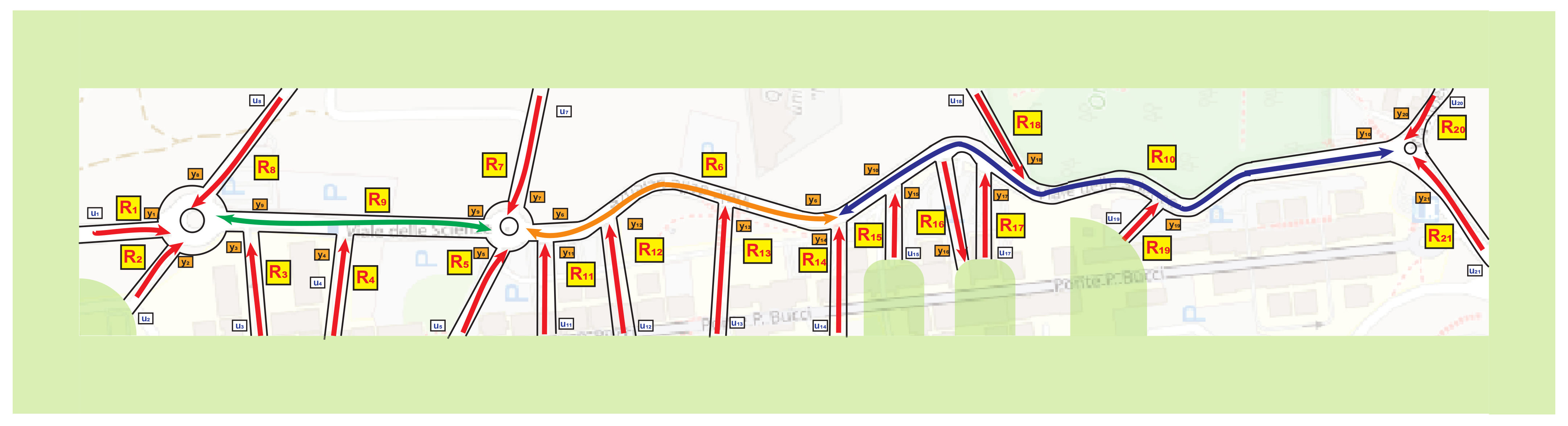
2. System Specifications and Problem Definition

A road network can be seen as a Wireless Sensor Network (WSN), where a collection of sensors like cameras, radar, and motion sensors provide traffic insights for each road sector. This section addresses the observability-based sensor selection issue, focusing on smart lighting, pollutant monitoring, and similar applications. The overarching design methodology is described, encompassing considerations of urban network topology and the state-space representation of the traffic model. This comprehensive approach facilitates the identification of potential sensor placement locations. Subsequently, a judiciously chosen minimum subset is selected to formulate the design of a state observer. This observer is tasked with providing accurate estimations of traffic flow within the specified urban area.

In summary, the system under consideration is a smart urban infrastructure incorporating a network of sensors, such as cameras, radar, and motion sensors. This network is designed to monitor vehicular traffic within distinct sectors of the road network. The ultimate goal is to leverage these traffic data for intelligent applications, particularly in the realm of smart lighting and traffic pollutant monitoring. The central challenge addressed in this study revolves around the observability-based sensor selection problem. Given the urban network’s topology and a state-space representation of the traffic model, the objective is to strategically position a subset of sensors within the network. This subset should be carefully chosen to optimize the design of a state observer capable of accurately estimating the traffic flow across the urban area. The key components of the problem are as follows:

• Urban network topology: the layout and connectivity of the urban road network, defining the spatial relationships between different sectors and links.
• State-space representation: a mathematical representation of the traffic model in state-space form, capturing the dynamics and interactions within the system.
• Sensor placement locations: identification of potential locations within the urban network where sensors (cameras, radar, motion sensors) can be strategically placed.
• Observer design: formulation of a state observer that utilizes the selected subset of sensors to estimate the traffic flow accurately.

The goal is to develop a sensor placement strategy that optimizes urban network coverage for traffic monitoring by carefully choosing sensors and designing an observer to improve system observability and provide accurate traffic estimates.

2.1. Model Design

A compartmental traffic model is a mathematical or conceptual representation used to analyze and understand the flow of traffic in a transportation system [29]. These models break down the transportation system into different compartments or segments, each representing a specific aspect of the overall traffic dynamics. The purpose of compartmental models is to simplify the complexity of real-world traffic systems for analysis and simulation. There are various types of compartmental traffic models, and they may focus on different aspects of traffic behavior. In general, it is possible to refer to three main categories of compartmental traffic models:

• Macroscopic traffic models encompass traffic flow models, which analyze overarching traffic patterns by considering factors like density, speed, and flow, often employing fluid dynamics’ principles for a macro-level perspective. They also include queuing models that investigate the dynamics of traffic queue formation and dissipation, focusing on critical points such as intersections, toll booths, and traffic signals.
• Mesoscopic traffic models examine traffic dynamics at an intermediate level. Link-based models focus on the specific dynamics of individual links or segments within a transportation network, capturing the traffic flow on particular road sections. Cell transmission models, on the other hand, segment the roadway into discrete cells, simulating vehicle movement from one cell to another while accounting for variables such as speed limits and traffic signals, offering a granular view of traffic behavior.
• Microscopic traffic models delve into the intricate behaviors of individual vehicles and drivers. Car-following models closely simulate the actions of individual vehicles, focusing on driver responses to preceding vehicles and including considerations such as acceleration, deceleration, and safe following distances. Meanwhile, agent-based models treat each driver as an independent decision-maker, exploring their unique decision-making processes, interactions with other drivers, and reactions to surrounding traffic conditions, providing a detailed analysis of driver behavior within the traffic system.

In what follows, a traffic compartment model is initially established following the approach outlined in [30]. The conceptual design of the compartmental model is straightforward: the system is divided into homogeneous compartments, and the flow between these compartments is tracked. For a more general discussion, refer to Figure 1, illustrating a basic example of a compartmental system. In this figure, the compartments (representing road sectors) are depicted as boxes, and the flows are indicated by arrows. Additionally, $u_i$ indicates the number of cars entering the ith road sector, while $y_i$ denotes the number of vehicles exiting the ith road sector ($i=1,\dots ,5$). It is important to note that some cars leaving the ith road sector may become an input for the jth road sector ($i=1,\dots ,5$, $j=1,\dots ,5$, $j\ne i$); for instance, $y_3$ becomes an input for $R_4$.

Figure 1 illustrates the structural configuration of the compartmental system, which can be visualized as a directed graph. In this representation, the compartments correspond to vertices, and the flows between them are depicted as arcs.

This paper presents a simplified traffic model using the following discrete-time Linear Time-Invariant (LTI) state-space framework:

$$\begin{array}{cc}\hfill x(t+1)& \hfill =Ax\left(t\right)+Bu\left(t\right),x\left(0\right)=x_0\hfill \end{array}$$

(1)

$$\begin{array}{cc}\hfill y\left(t\right)& \hfill =Cx\left(t\right)+Du\left(t\right)\hfill \end{array}$$

(2)

where $x\left(t\right)\in {\mathbb{R}}^n$ is the system state, $u\left(t\right)\in {\mathbb{R}}^m$ is the system input, $y\left(t\right)\in {\mathbb{R}}^p$ is the measurable output, A, B, C, and D are matrices with appropriate dimensions. In the road network model, $x_i\left(t\right)$ represents the number of vehicles in the ith compartment, assuming each compartment meets the specified condition:

$$x_i\left(t\right)\ge 0,\forall t\ge 0$$

(3)

The flow $f_{ji}$ from the ith to the jth compartment is proportional to $x_i\left(t\right)$, dictated by a non-negative constant splitting ratio $a_{ji}$:

$$f_{ji}=a_{ji}{x}_i\left(t\right),j\ne i,a_{ji}\ge 0$$

(4)

The compartmental road network is modeled as an LTI system, Equations (1) and (2) [26], in which the system state $x\left(t\right)\in {\mathbb{R}}^n$ is defined such that $x_i\left(t\right)$ denotes the traffic flow (vehicles per unit time) in the ith road sector; the elements of the state matrix $A\in {\mathbb{R}}^{n\times n}$ represent splitting ratios, determined by the roads’ importance ranks from OSM; the system input $u\left(t\right)$ is such that $u_i$ indicates the number of cars entering the ith road sector; the system output $y\left(t\right)$ is defined such that $y_i\left(t\right)$ indicates the number of vehicles exiting the ith road sector. Further details about the model definition can be found in [23].

 Remark 1. 

It is important to highlight that although the traffic flow is not well described by LTI dynamical models, here, it is supposed to work on a specific equilibrium point, where linearization procedures can be applied [26].

2.2. Improving the Model

In order to enhance the quality of the adopted model (1) and (2) and make it applicable in a real case study, it is necessary to use identification techniques that can reduce the error between the model and real data. Prediction error minimization (PEM) is a method that uses optimization to reduce the error between the output of the model and the measurement data. In this respect, the PEM algorithm must have knowledge of the mathematical structure of the model. This includes understanding parameters such as matrix elements in the state-space model (1) and (2), allowing for an effective optimization. The problem is defined in the form of a cost function that includes the error between the model and the predicted output. PEM employs a numerical optimization to minimize the cost function, which is a weighted norm of the prediction error. PEM is defined as follows for scalar outputs:

$$V_N(G,H)=\sum _{t=1}^N{e}^2\left(t\right)$$

(5)

where $e\left(t\right)$ is the difference between the measured output and the predicted output of the model. We introduce the backward shift operator $q^{-1}$:

$$q^{-1}u\left(t\right)=u(t-1)$$

(6)

so that the linear model can be written as

$$y\left(t\right)=G\left(q\right)u\left(t\right)+H\left(q\right)e\left(t\right)$$

(7)

where

$$G\left(q\right)=\sum _{i=1}^{\infty }g\left(i\right)q^{-i};H\left(q\right)=\sum _{i=1}^{\infty }h\left(i\right)q^{-i}.$$

(8)

are the transfer functions of the linear system in (7). For the linear model in (7), the error is defined as:

$$e\left(t\right)=H^{-1}\left(q\right)\left[y\left(t\right)-G\left(q\right)u\left(t\right)\right]$$

(9)

Note that:

• $e\left(t\right)$ is a vector;
• The cost function $V_N(G,H)$ is a scalar value;
• The subscript N means that the cost function is dependent on the number of data samples and becomes more accurate as N increases.

Further details about PEM can be found in [31].

2.3. Observability Metric

Observability, a key structural property of dynamic systems, pertains to the ability to estimate the initial state $x\left(t_0\right)$ using given data $\left(u\right(t),y(t\left)\right)$ for all $t\ge t_0$ and $t_0\ge 0$. This property is satisfied if and only if the observability matrix

$$\mathcal{O}={\left[\begin{array}{c}{C}^T,{\left(CA\right)}^T,\dots ,{\left(C{A}^{n-1}\right)}^T\end{array}\right]}^T$$

(10)

has full $rank\left(\mathcal{O}\right)=n$. The observability matrix (10) falls short for the sensor selection problem as it merely offers a binary “on/off” indication without insights into the quality of observability. A more appropriate performance criterion for observability involves employing the condition number of W:

$$\mathcal{K}\left(W\right)=\frac{\overline{\sigma }\left(W\right)}{\underline{\sigma }\left(W\right)}$$

(11)

where

• W is the observability Gramian defined as

  $$W=\sum _{k=1}^{n-1}{\left(A^T\right)}^k{C}^{T}C{A}^k$$

  (12)
• $\overline{\sigma }\left(W\right)$ and $\underline{\sigma }\left(W\right)$ represent the largest and smallest singular values of the observability Gramian, respectively.

It is noteworthy that the Gramian’s association with the energy of the natural response, triggered by the initial state $x\left(0\right)$, implies that a higher energy level enhances the observability of the initial state. In particular [26],

• The trace of the Gramian $tr\left(W\right)$ is directly related to the average energy and can be interpreted as the average observability in all directions in the state space.
• In Equation (11), the smallest singular value $\underline{\sigma }\left(W\right)$ of the Gramian is related to the energy of the least observable mode, while the largest $\overline{\sigma }\left(W\right)$ is related to the energy of the most observable one; hence, the condition number K measures how balanced the observability is among all the modes.
• The rank of the Gramian $rank\left(W\right)$ is the dimension of the observable subspace.

Moreover, the eigenvalues/vectors of the observability Gramian W provides much information on the quality of the state reconstruction error as a function of sensor placement and selection. In particular, the minimum eigenvalue of this matrix is critical and should not be too small to avoid large reconstruction errors. Among various ways to measure the “size” of W, a recent study [26] suggests to use the condition number as a performance sensor selection criterion because it usually leads to a smaller number of sensors selected than other criteria, such as the trace or the rank of W.

2.4. Problem Definition

Consider a designated monitoring area $\mathcal{T}$, with $\mathcal{R}$ representing the main roads within $\mathcal{T}$. Utilizing the road network model (1) and (2), and the condition number (11) as an observability metric, we define $\mathcal{S}$ as the set of all n potential sensor locations, where each ${\xi }_i\in \mathcal{S}$ corresponds to the ith sensor position. The goal is to develop a sensor selection strategy that identifies a minimal subset of p sensors from the n available locations, optimizing the performance criterion (11) and ensuring system observability.

3. Observability-Based Sensor Selection

Within the framework of the road network model (1) and (2), the sensor selection process aims to find a subset $\mathcal{J}\subseteq \mathcal{S}$, containing p sensors from the n available, to enhance observability. Thus, the challenge of selecting sensors based on observability is tackled by optimizing the observability Gramian. The sensor selection issue is framed as solving a mixed-integer constrained optimization problem, as detailed in [10]:

$$\begin{array}{cc}\hfill & \hfill \underset{\beta }{min}\mathcal{K}\left[W\left(\beta \right)\right]\hfill \\ \hfill s.t.& \hfill \sum _{i=1}^n{\beta }_i=p\hfill \\ \hfill & \hfill {\beta }_i\in \left\{0,1\right\},i=1\dots ,n\hfill \end{array}$$

(13)

In this context, $\mathcal{K}[·]$ represents a convex scalar measure of the observability Gramian, such as the condition number, as outlined in [10]. Furthermore, the budget constraint (13) mandates the selection of precisely p sensors. It is important to emphasize that in the context of the sensor selection problem being addressed, we have the following:

• Referring to the model (1), the subsequent output equation is taken into account.

  $$y^{*}\left(t\right)=C\left(\mathcal{J}\right)x\left(t\right)$$

  (14)

  in which $C\left(\mathcal{J}\right)\in {\mathbb{R}}^{p\times n}$ represents the matrix corresponding to the road sectors where sensors are to be installed, comprising p rows selected from the $n\times n$ identity matrix based on the index set $\mathcal{J}={\xi }_1,\dots ,{\xi }_p$.
• The observability Gramian (12) is thus reformulated as

  $$W\left(\beta \right)=\sum _{i=1}^n{\beta }_i\sum _{k=1}^{n-1}{\left(A^T\right)}^{k}C{\left(\mathcal{J}\right)}^{T}C\left(\mathcal{J}\right)A^k$$

  (15)

  where ${\beta }_i$, $i=1,\dots ,n$ (where n is the maximum number of streets contained in the road network, or equivalently, the maximum number of sensors that can be installed) are binary “‘activation variables”’ whose meaning can be summarized by the function

  $$\Lambda \left(\mathcal{J}\right)=\left\{\begin{array}{c}{\beta }_i=1,\mathrm{the}\mathrm{sensor}{\xi }_i\mathrm{is}\mathrm{selected}\hfill \\ \hfill {\beta }_i=0,\mathrm{the}\mathrm{sensor}{\xi }_i\mathrm{is}\mathrm{NOT}\mathrm{selected}\hfill \end{array}\right.$$

  (16)

The optimization problem (13) is inherently combinatorial, requiring the selection of a finite set of sensor locations that meet certain criteria. While the exhaustive search method (also known as brute-force method) can identify the global optimum ${\mathcal{S}}^{opt}$ by evaluating all combinations, its NP-hard nature and high computational complexity make it impractical for large networks. Therefore, more practical, albeit suboptimal, strategies like heuristic procedures are recommended to find a suitable sensor set ${\mathcal{S}}^{*}\subseteq S$ with $\left|{\mathcal{S}}^{*}\right|=p$, acknowledging that these methods may not guarantee the optimal selection. Due to the problem’s nonlinear, non-convex characteristics, using global optimization solvers like simulated annealing (SA) and genetic algorithms is crucial for identifying feasible solutions. These heuristic outcomes are then compared with those from exhaustive searches to evaluate their effectiveness.

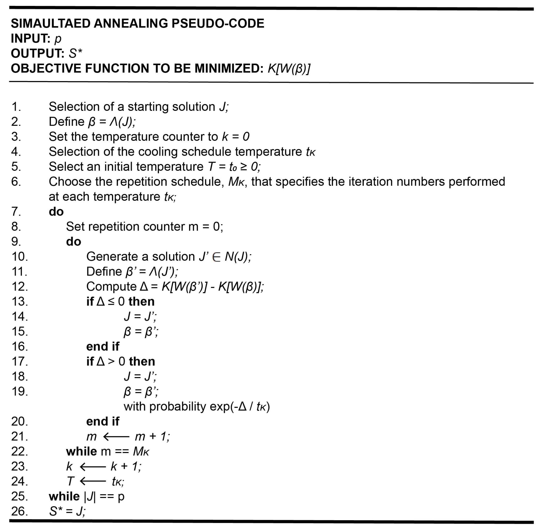
4. Simulated Annealing Heuristic

SA is a local search algorithm employed for seeking a global optimum within a vast search space, particularly in optimization problems with discrete solutions. Its name draws an analogy from the metallurgical process of annealing, involving the controlled heating and cooling of solids. Unlike classical local search algorithms, such as gradient descent, which may get stuck in local minima, SA aims to mitigate this risk by occasionally accepting moves that increase the cost, thus exploring a broader solution space [27].

In the context of discrete optimization problems, each iteration of the simulated annealing procedure involves comparing the values of two solutions: the current solution and a newly selected one. While improving solutions are always accepted, a fraction of non-improving (inferior) solutions is also accepted. This acceptance of non-improving solutions is a strategic move to avoid getting stuck in local optima and enhances the algorithm’s chances of finding a global optimum. The probability of accepting non-improving solutions is governed by a temperature parameter, which typically decreases at each iteration of the procedure. As the temperature drops, the likelihood of accepting suboptimal solutions decreases, allowing the algorithm to gradually converge towards an optimal solution.

To outline the simulated annealing (SA) algorithm, the following components are introduced:

• The solution space $\Omega$ (i.e., the set of all possible solutions):

  $$\Omega =\left\{\mathcal{J}\subseteq \mathcal{S}:rank\left(W\right(\beta \left)\right)=n;\beta =\Lambda \left(\mathcal{J}\right)\right\}$$

  (17)
• The objective function $\mathcal{K}\left[W\right(\beta \left)\right]$ defined on the solution space.

The objective is to identify the global minimum, ${\mathcal{S}}^{*}$, such that ${\mathcal{S}}^{*}\subseteq \Omega$ and $\mathcal{K}\left[W\left({\beta }^{*}\right)\right]\le \mathcal{K}\left[W\left(\beta \right)\right]$ for every $\mathcal{J}\in \Omega$. Define $N\left(\mathcal{J}\right)$ as the neighborhood set of $\mathcal{J}$, implying that for each solution $\mathcal{J}\in \Omega$, there exist neighboring solutions ${\mathcal{J}}^{\prime }\in N\left(\mathcal{J}\right)$ accessible in one local search iteration. The SA algorithm initiates with a solution $\mathcal{J}\in \Omega$, generating a neighboring solution ${\mathcal{J}}^{\prime }\in N\left(\mathcal{J}\right)$ through random selection or a defined rule. The transition from the current solution $\mathcal{J}$ to a candidate ${\mathcal{J}}^{\prime }$ follows the Metropolis acceptance criterion, which simulates thermodynamic transitions aiming to minimize energy. The acceptance of ${\mathcal{J}}^{\prime }$ as the new current solution is determined by a specified acceptance probability:

$$P\left({\mathcal{J}}^{\prime }\right)=\left\{\begin{array}{cc}exp(-(\Delta /t_k))& if\Delta >0\\ 1& otherwise\end{array}\right.$$

(18)

The acceptance probability is calculated using $\Delta =\mathcal{K}\left[W\left({\beta }^{\prime }\right)\right]-\mathcal{K}\left[W\left(\beta \right)\right]$, where $\Delta$ represents the change in the performance measure due to the transition from the current solution $\beta$ to a candidate solution ${\beta }^{\prime }$. The parameter $t_k$

$$t_k:=\left\{t_k>0,\forall k,\underset{k\to \infty }{lim}{t}_k=0\right\}$$

(19)

denotes the “temperature” at iteration k, influencing the likelihood of accepting solutions with higher $\Delta$ values, thereby allowing exploration of the solution space and aiding in avoiding local minima.

This acceptance probability is the basic element of the search mechanism in simulated annealing. If the temperature is reduced sufficiently slowly, then the system can reach an equilibrium (steady state) at each iteration k. Let $\mathcal{K}\left[W\right(\beta \left)\right]$ and $\mathcal{K}\left[W\left({\beta }^{\prime }\right)\right]$ denote the energies (objective function values) associated with solutions $\mathcal{J}\in \Omega$ and ${\mathcal{J}}^{\prime }\in N\left(\mathcal{J}\right)$, respectively. This equilibrium follows the Boltzmann distribution, which can be described as the probability of the system being in state $\mathcal{J}\in \Omega$ with energy $\mathcal{K}\left[W\right(\beta \left)\right]$ at temperature T, such that the probability the system is in state $\mathcal{J}$ at temperature T is

$$P(\mathcal{J},T)=\frac{exp(-\mathcal{K}\left[W\left(\beta \right)\right]/t_k)}{{\sum }_{{\mathcal{J}}^{″}\in \Omega exp\left(\mathcal{K}\left[W\left(\beta \right)\right]\right)/t_k)}}$$

(20)

for all possible neighbor solutions ${\mathcal{J}}^{\prime \prime }\in N\left(\mathcal{J}\right)$. If the probability of generating a candidate solution ${\mathcal{J}}^{\prime }$ from the neighbors of solution $\mathcal{J}\in \Omega$ is $g_k(\mathcal{J},{\mathcal{J}}^{\prime })$ where

$$\sum _{{\mathcal{J}}^{\prime }\in N\left(\mathcal{J}\right)g_k(\mathcal{J},{\mathcal{J}}^{\prime })}=1,\forall \mathcal{J}\in \Omega ,k=1,2,\dots ,$$

(21)

then a non-negative, square, stochastic matrix ${\mathbf{P}}_k$ can be defined with transition probabilities

$${\mathbf{P}}_k(\mathcal{J},{\mathcal{J}}^{\prime })\left\{\begin{array}{ccc}{g}_k(\mathcal{J},{\mathcal{J}}^{\prime })exp(-{\Delta }_{\mathcal{J},{\mathcal{J}}^{\prime }}/t_k)& {\mathcal{J}}^{\prime }\in N\left(\mathcal{J}\right)& {\mathcal{J}}^{\prime }\ne \mathcal{J}\\ 0& {\mathcal{J}}^{\prime }\notin N\left(\mathcal{J}\right)& {\mathcal{J}}^{\prime }\ne \mathcal{J}\\ 1-\sum _{{\mathcal{J}}^{″}\in N\left(\mathcal{J}\right),{\mathcal{J}}^{\prime \prime }\ne \mathcal{J}}{\mathbf{P}}_k(\mathcal{J},{\mathcal{J}}^{\prime \prime })& {\mathcal{J}}^{\prime }=\mathcal{J}\end{array}\right.$$

(22)

for all solutions $\mathcal{J}\in \Omega$, all iterations $k=1,2,\dots$, and with ${\Delta }_{\mathcal{J},{\mathcal{J}}^{\prime }}=\mathcal{K}\left[W\left({\beta }^{\prime }\right)\right]-\mathcal{K}\left[W\left(\beta \right)\right]$.

Note that this formulation for simulated annealing requires executing a total of $M_0+\dots +M_k$ iterations, where k is the value of $t_k$ at which a stopping criterion is met (e.g., a pre-specified total number of iterations or a solution of a certain quality has been found). If $M_k=1$ for all k, the temperature changes at each iteration. The SA pseudocode referring to the sensor selection procedure is reported in Figure 2.

 Remark 2. 

The solution of the optimization problem (13) can be easily obtained by customizing the built-in MATLAB 2021a function simulannealbnd that allows one to find the minimum of a function using the simulated annealing algorithm.

5. Genetic Algorithms

GA reproduces the evolutionary behavior of biological systems [32]. GA provides a population (also called generation) of candidate solutions to an underlying optimization problem, which is evolved toward better solutions. The GA template used for the sensor selection purpose is reported in Figure 3. Each generation has a set of properties which can be mutated and altered. Genetic algorithms are designed to search the optimal solution via weeding out the worst gene strings (individual) based on a fitness function that is usually defined as the value of the objective function of the optimization problem being solved [33]. In particular, an iterative process involving an initial population of randomly generated individuals (e.g., an initial set of sensors) transforms each population of candidate solutions into a descendant population. At each iteration, the fitness of every individual (e.g., sensor) belonging to the generation is evaluated. The fitter individuals are stochastically selected from the current population, and each individual’s genome is modified to form a new generation. The new generation of candidate solutions is then used in the next iteration of the algorithm. The algorithm ends when either a maximum number of generations has been produced or a satisfactory fitness level has been reached.

 Remark 3. 

The solution of the optimization problem (13) can be easily obtained by properly using the built-in MATLAB function ga that allows one to find the minimum of a function using a genetic algorithm.

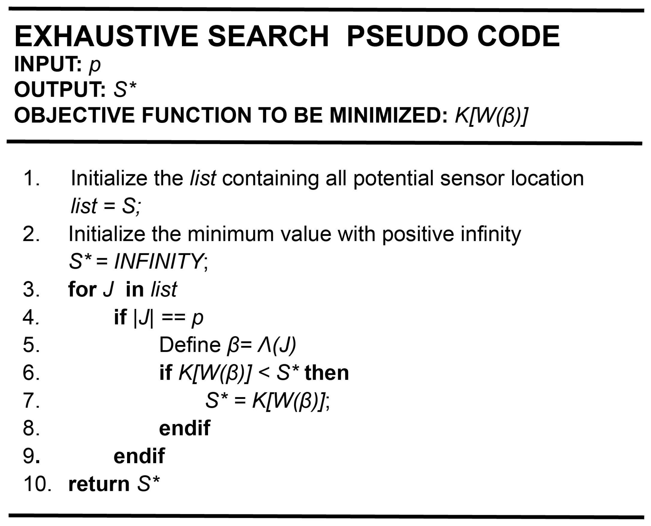
6. Exhaustive Search Algorithms

An exhaustive search algorithm is a method used to find the optimal solution to a problem by systematically exploring all possible solutions. It works by considering every possible combination of solutions within a given search space [34]. A brief description of the steps involved in an exhaustive search algorithm is as follows:

• Generate candidates: create a list of all possible solutions within the defined search space.
• Evaluate candidates: evaluate the objective function or cost associated with each candidate solution.
• Select optimal solution: identify the solution with the minimum or maximum objective function value, depending on whether you are minimizing or maximizing.
• Repeat: continue this process until all possible solutions have been considered.

While exhaustive search guarantees finding the optimal solution, it can be computationally expensive, especially for large search spaces, as it explores every combination. As a result, it may not be the most efficient approach for complex problems, and more sophisticated algorithms like dynamic programming or heuristic methods are often preferred for larger-scale optimization tasks. Figure 4 reports an example of pseudocode for an exhaustive search algorithm to find the minimum value of condition number $\mathcal{K}\left[W\right(\beta \left)\right]$ in a list of possible sensor configurations. In particular, this pseudocode represents a basic algorithm that goes through each element in a list, compares it with the current minimum value, and updates the minimum value if a smaller element is found.

7. Results

This section demonstrates the feasibility of the proposed simulated annealing-based sensor selection method through a case study that accounts for a traffic network comprising 21 road sections (a road layout around the University of Calabria), $\mathcal{R}=R_1,\dots ,R_{21}$, as depicted in Figure 5.

The initial phase involved establishing the road network model (1) and (2), which entailed calculating the state matrices A, B, C, and D. A solution to the sensor selection problem was obtained by properly customizing the built-in MATLAB functions simulannealbnd for integer/discrete optimization. This was accomplished by truncating generated floating-point numbers within sensible integral windows [35]. With $n=21$, the problem remained manageable, and we successfully identified the minimal subset ${\mathcal{S}}_{sa}^{*}$ within $\mathcal{S}$ that guaranteed the complete observability of the system (1)–(14):

$$\begin{array}{ccc}\hfill rank\left(O(A,C\left({\mathcal{S}}_{sa}^{*}\right))\right)\hfill & =& \hfill 21\hfill \end{array}$$

(23)

Specifically, for the accounted case study, the solution to the simulated-annealing sensor selection problem yielded the following results:

• Computation time (i.e., the duration required to execute the sensor selection algorithm and obtain the solution): 94.5 [s].
• Cardinality $\left|S_{sa}^{*}\right|=6$;
• $\mathcal{K}\left(W\right)=4.1102\times {10}^3$.
• ${\mathcal{S}}_{sa}^{*}=\left[{\xi }_3,{\xi }_{13},{\xi }_{15},{\xi }_{17},{\xi }_{19},{\xi }_{20}\right]$.

Additional tests were conducted to determine whether the solution obtained from the simulated annealing (SA) process was the smallest possible sensor set ensuring system observability. For this purpose, two approaches were examined: (1) a genetic algorithm (GA) sensor selection method as described in [26], and (2) a brute-force (exhaustive) search. The GA approach yielded the following outcomes:

• Computation time (i.e., the duration required to execute the sensor selection algorithm and obtain the solution): 89.6 [s].
• Cardinality $\left|S_{ga}^{*}\right|=7$;
• $\mathcal{K}\left(W\right)=7.6840\times {10}^4$.
• ${\mathcal{S}}_{ga}^{*}=\left[{\xi }_3,{\xi }_5,{\xi }_{12},{\xi }_{15},{\xi }_{17},{\xi }_{19},{\xi }_{20}\right]$.

On the other hand, Table 1 reports the exhaustive search outcomes. Recall that the exhaustive search procedure systematically checks every possible candidate to reliably find solutions to problems with a limited set of options. With reference to our case study in Table 1, we highlight several key points:

• The exhaustive search identified 12 sensor sets that ensured system observability;
• These solutions exhibited varying condition numbers (11);
• Sensor set number three coincided with the simulated annealing (SA) procedure’s solution and had the lowest condition number $\mathcal{K}\left(W\right)$ value, indicating optimal observability.

The results obtained indicated that both simulated annealing (SA) and genetic algorithm (GA) procedures were effective in identifying a sensor set that ensured system observability. The primary distinction between them lay in the cardinality of the sensor set and the computation time. Notably, the simulated annealing procedure tended to identify a smaller sensor set compared to the genetic algorithm, albeit at the cost of a slightly longer computational time (approximately +5% compared to the genetic algorithm). In the context of our case study, this difference was deemed acceptable. However, in more extensive application scenarios with a substantial number of sensors to be considered, the selection of an efficient local search heuristic becomes critical. The trade-off between sensor set size and computational efficiency should be carefully considered for larger-scale applications to ensure an optimal and practical solution.

Table 1. Sensor sets determined through exhaustive search procedure.

#	Sensor Sets	$\mathcal{K}\left(\mathit{W}\right)$
1	$\left[{\xi }_3,{\xi }_{13},{\xi }_{16},{\xi }_{17},{\xi }_{19},{\xi }_{20}\right]$	$4.1208\times {10}^3$
2	$\left[{\xi }_3,{\xi }_{12},{\xi }_{16},{\xi }_{17},{\xi }_{19},{\xi }_{20}\right]$	$4.1509\times {10}^3$
3	$\left[{\xi }_3,{\xi }_{13},{\xi }_{15},{\xi }_{17},{\xi }_{19},{\xi }_{20}\right]$	$4.1102\times {10}^3$
4	$\left[{\xi }_3,{\xi }_{12},{\xi }_{15},{\xi }_{17},{\xi }_{19},{\xi }_{20}\right]$	$4.1509\times {10}^3$
5	$\left[{\xi }_3,{\xi }_{13},{\xi }_{15},{\xi }_{16},{\xi }_{19},{\xi }_{20}\right]$	$4.1719\times {10}^3$
6	$\left[{\xi }_3,{\xi }_{12},{\xi }_{15},{\xi }_{16},{\xi }_{19},{\xi }_{20}\right]$	$4.1891\times {10}^3$
7	$\left[{\xi }_3,{\xi }_{13},{\xi }_{16},{\xi }_{17},{\xi }_{18},{\xi }_{20}\right]$	$4.2209\times {10}^3$
8	$\left[{\xi }_3,{\xi }_{12},{\xi }_{16},{\xi }_{17},{\xi }_{18},{\xi }_{20}\right]$	$4.3519\times {10}^3$
9	$\left[{\xi }_3,{\xi }_{13},{\xi }_{15},{\xi }_{17},{\xi }_{18},{\xi }_{20}\right]$	$4.1369\times {10}^3$
10	$\left[{\xi }_3,{\xi }_{12},{\xi }_{15},{\xi }_{17},{\xi }_{18},{\xi }_{20}\right]$	$4.1869\times {10}^3$
11	$\left[{\xi }_3,{\xi }_{13},{\xi }_{15},{\xi }_{16},{\xi }_{18},{\xi }_{20}\right]$	$4.4511\times {10}^3$
12	$\left[{\xi }_3,{\xi }_{12},{\xi }_{15},{\xi }_{16},{\xi }_{18},{\xi }_{20}\right]$	$4.1519\times {10}^3$

Table 1. Sensor sets determined through exhaustive search procedure.

#	Sensor Sets	$\mathcal{K}\left(\mathit{W}\right)$
1	$\left[{\xi }_3,{\xi }_{13},{\xi }_{16},{\xi }_{17},{\xi }_{19},{\xi }_{20}\right]$	$4.1208\times {10}^3$
2	$\left[{\xi }_3,{\xi }_{12},{\xi }_{16},{\xi }_{17},{\xi }_{19},{\xi }_{20}\right]$	$4.1509\times {10}^3$
3	$\left[{\xi }_3,{\xi }_{13},{\xi }_{15},{\xi }_{17},{\xi }_{19},{\xi }_{20}\right]$	$4.1102\times {10}^3$
4	$\left[{\xi }_3,{\xi }_{12},{\xi }_{15},{\xi }_{17},{\xi }_{19},{\xi }_{20}\right]$	$4.1509\times {10}^3$
5	$\left[{\xi }_3,{\xi }_{13},{\xi }_{15},{\xi }_{16},{\xi }_{19},{\xi }_{20}\right]$	$4.1719\times {10}^3$
6	$\left[{\xi }_3,{\xi }_{12},{\xi }_{15},{\xi }_{16},{\xi }_{19},{\xi }_{20}\right]$	$4.1891\times {10}^3$
7	$\left[{\xi }_3,{\xi }_{13},{\xi }_{16},{\xi }_{17},{\xi }_{18},{\xi }_{20}\right]$	$4.2209\times {10}^3$
8	$\left[{\xi }_3,{\xi }_{12},{\xi }_{16},{\xi }_{17},{\xi }_{18},{\xi }_{20}\right]$	$4.3519\times {10}^3$
9	$\left[{\xi }_3,{\xi }_{13},{\xi }_{15},{\xi }_{17},{\xi }_{18},{\xi }_{20}\right]$	$4.1369\times {10}^3$
10	$\left[{\xi }_3,{\xi }_{12},{\xi }_{15},{\xi }_{17},{\xi }_{18},{\xi }_{20}\right]$	$4.1869\times {10}^3$
11	$\left[{\xi }_3,{\xi }_{13},{\xi }_{15},{\xi }_{16},{\xi }_{18},{\xi }_{20}\right]$	$4.4511\times {10}^3$
12	$\left[{\xi }_3,{\xi }_{12},{\xi }_{15},{\xi }_{16},{\xi }_{18},{\xi }_{20}\right]$	$4.1519\times {10}^3$

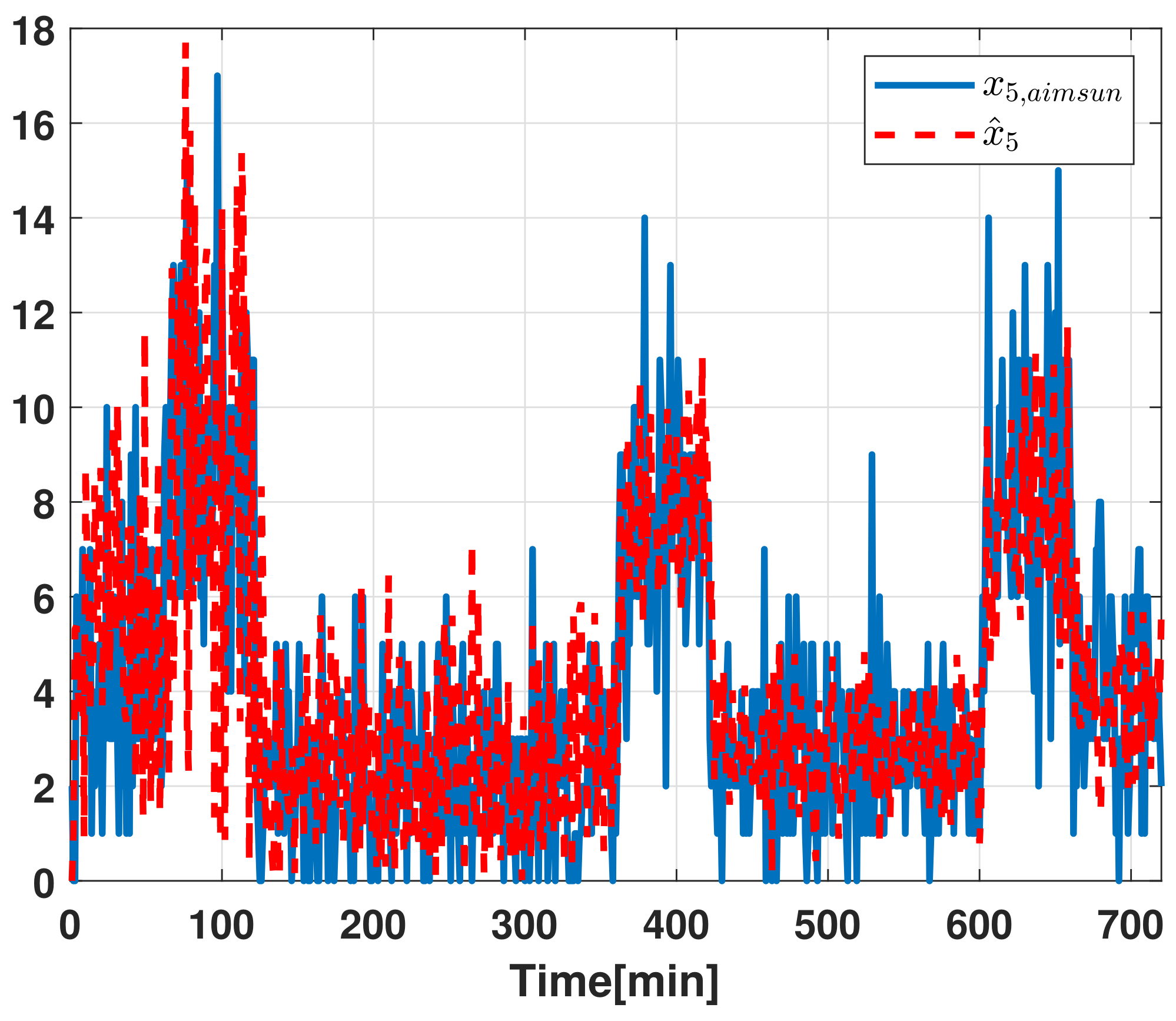
7.1. State Reconstruction Error

Luenberger state observers were configured for sensor sets $\left(S_{sa}^{*}\right)$ and $\left(S_{ga}^{*}\right)$ to compare their state (traffic flow) reconstruction accuracy. The design of observer matrix gains in the $H_2$ sense minimized the expected mean-square error (MSE) in response to a white-noise input, acknowledging sensor data could be distorted by exogenous disturbance $v\left(t\right)=WN(0,\sigma )$. The analysis, considering traffic inputs $u_i\left(t\right)$ for $i=1,\dots ,21$ as illustrated in Figure 6, noted that inputs for sectors $R_6$, $R_9$, $R_{10}$, and $R_{16}$ were zero due to their disconnection from external roads. Figure 7 reports the traffic estimation provided by the two Luenberger state observers configured for sensor sets $\left(S_{sa}^{*}\right)$ and $\left(S_{ga}^{*}\right)$, respectively. In particular, Figure 7 delves into the evolution of states ($x_1$, $x_2$, $x_{12}$, $x_{18}$) under these inputs, contrasting true states (blue line) with estimates from $\left(S_{sa}^{*}\right)$ (green dashed line) and $\left(S_{ga}^{*}\right)$ (red dashed line), highlighting the superior accuracy of $\left(S_{sa}^{*}\right)$’s estimates. Note that for the sake of clarity, Figure 7 refers to the first 100 [s] of the simulation. This pattern of superior estimation accuracy by $\left(S_{sa}^{*}\right)$ extended to all system states ($x_i$, $i=1,\dots ,21$, $i\ne 1,2,12,18$).

Further analysis were performed by considering two error metrics: the mean absolute error (MAE), a measure of errors between paired observations expressing the same phenomenon, and the root-mean-square error (RMSE), which shows how far predictions fall from measured true values using the Euclidean distance. Furthermore, Figure 8 and Figure 9 present the MAE and RMSE of state reconstructions, respectively, computed across the entire simulation period for all states ($x_i$), providing a comprehensive evaluation of observer performance. In particular, from these two figures, it is evident that the MAE (mean absolute error) and the RMSE (root-mean-square error) were always lower in the case of traffic flow reconstruction obtained through the design of a Luenberger observer based on the sensor set calculated via simulated annealing. The results demonstrate that the observer configured for the sensor set $\left(S_{sa}^{*}\right)$ achieved superior performance compared to the observer designed for the sensor set $\left(S_{ga}^{*}\right)$.

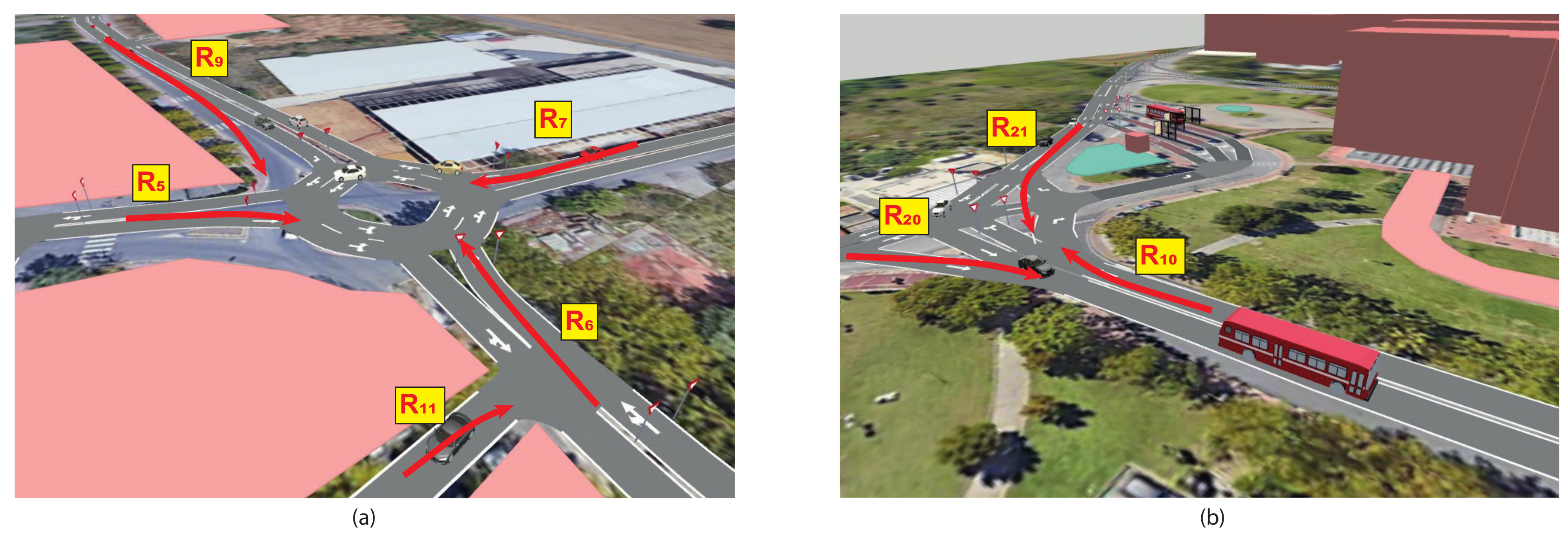
7.2. Validation

To validate the presented approach, a further study was performed by accounting Aimsun Next which is a traffic simulation software designed for modeling and analyzing transportation systems [36]. Developed by TSS-Transport Simulation Systems, Aimsun Next is widely used by transportation engineers, planners, and researchers to simulate and evaluate the performance of traffic networks. Here are some key features and aspects of Aimsun Next:

• Microsimulation: Aimsun Next uses microsimulation, allowing for a detailed modeling of individual vehicles and their interactions within a traffic network. This level of detail is crucial for understanding how traffic behaves in various scenarios.
• Network modeling: the software enables users to create realistic models of road networks, including various types of intersections, signalized and unsignalized junctions, and different road types.
• Traffic demand modeling: Aimsun Next can simulate various traffic demand scenarios, helping users analyze the impact of changes in demand on the transportation system. This includes different modes of transportation such as private vehicles, public transit, pedestrians, and cyclists.
• Dynamic traffic assignment (DTA): the software supports dynamic traffic assignment, allowing for the modeling of real-time traffic conditions and the dynamic adaptation of routes by individual vehicles based on changing conditions.
• Simulation output and analysis: Aimsun Next provides detailed output data, including traffic flow, travel times, delays, and other performance metrics. This information helps users assess the effectiveness of different traffic management strategies and infrastructure improvements.
• Calibration and validation: the software allows users to calibrate and validate their models against real-world data, ensuring that the simulation results accurately reflect the observed behavior of the transportation system.
• Pollutant emission evaluation: Aimsun Next can model pollutant emissions for all vehicles in the simulation. The vehicle state (idling, cruising, accelerating, or decelerating) and the vehicle speed/acceleration are used to evaluate the emission from each vehicle for each simulation time step. This is done by referencing look-up tables for each pollutant, which give emissions for every relevant combination of vehicle behaviors and speed/acceleration.
• Integration with other tools: Aimsun Next may offer integration capabilities with other transportation planning and modeling tools, allowing for a more comprehensive analysis of the entire transportation planning process.

In reference to our case study (the road layout around the University of Calabria), the Aimsun Next software was utilized to generate a digital twin, as depicted in Figure 10a,b for the road network shown in Figure 5. The validation of the proposed architecture involved two primary steps. Firstly, an identification procedure was established to recognize the traffic model (1) and (2) based on the traffic data supplied by the designed digital-twin traffic network. This identification process utilized the prediction error minimization (PEM) algorithm, which refines linear and nonlinear models provided by the Matlab System Identification Toolbox. The PEM algorithm was specifically employed to update the matrices A, B, C, and D of the initial model (1) and (2). Secondly, the SA procedure was applied to determine the subset of sensors ${\mathcal{S}}^a$ for use. Notably, the same sensor subset ${\mathcal{S}}^a$ identified in Section 7 was obtained. Finally, the subset ${\mathcal{S}}^a$ was used to design the $H_2$ Luenberger state observer in charge of providing the estimation of the system state.

The validation process encompassed a 12 h traffic data collection test. The results of the validation test are showcased in Figure 11, Figure 12 and Figure 13 and

Table 2. Experimental validation using Aimsun Next software: traffic flow estimation quality evaluated via root-mean-square errors.

${\mathbf{e}}_1$	3.9	${\mathbf{e}}_8$	3.2	${\mathbf{e}}_{15}$	1.9
${\mathbf{e}}_{\mathbf{2}}$	2.6	${\mathbf{e}}_{\mathbf{9}}$	9.4	${\mathbf{e}}_{\mathbf{16}}$	1.4
${\mathbf{e}}_{\mathbf{3}}$	0.1	${\mathbf{e}}_{\mathbf{10}}$	0.5	${\mathbf{e}}_{\mathbf{17}}$	0.7
${\mathbf{e}}_{\mathbf{4}}$	1.6	${\mathbf{e}}_{\mathbf{11}}$	1.5	${\mathbf{e}}_{\mathbf{18}}$	0.7
${\mathbf{e}}_{\mathbf{5}}$	2.9	${\mathbf{e}}_{\mathbf{12}}$	0.9	${\mathbf{e}}_{\mathbf{19}}$	5.7
${\mathbf{e}}_{\mathbf{6}}$	4.6	${\mathbf{e}}_{\mathbf{13}}$	1.2	${\mathbf{e}}_{\mathbf{20}}$	0.2
${\mathbf{e}}_{\mathbf{7}}$	2.7	${\mathbf{e}}_{\mathbf{14}}$	1.5	${\mathbf{e}}_{\mathbf{21}}$	13.7

, where the traffic flow estimation capabilities and root-mean-square errors are reported, respectively. Specifically, the figures compare the system state (traffic flow) estimation (${\widehat{x}}_1$, ${\widehat{x}}_2$, and ${\widehat{x}}_5$) obtained using the sensor subset ${\mathcal{S}}^a$ (red dashed line) with the Aimsun Next data ($x_{1,aimsun}$, $x_{2,aimsun}$, and $x_{5,aimsun}$—blue line). Finally, Table 2 presents the root-mean-square errors computed over the 12 h test period. The obtained results confirm the satisfactory performance of the proposed estimation architecture in this scenario.

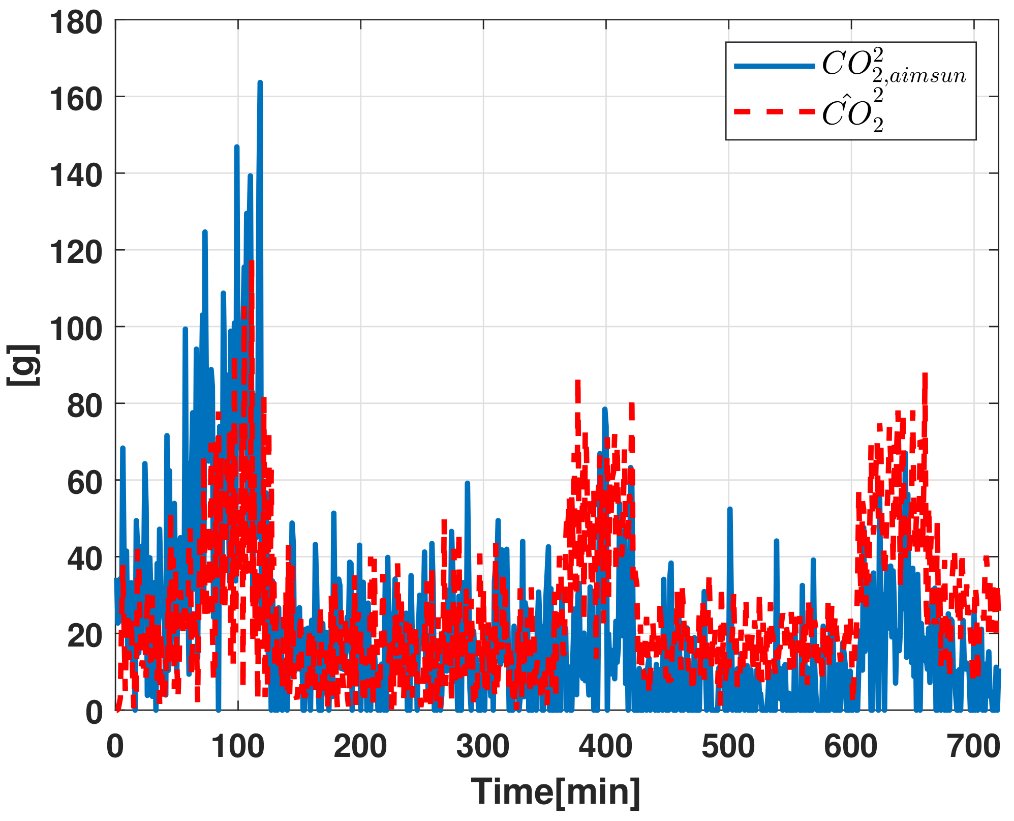
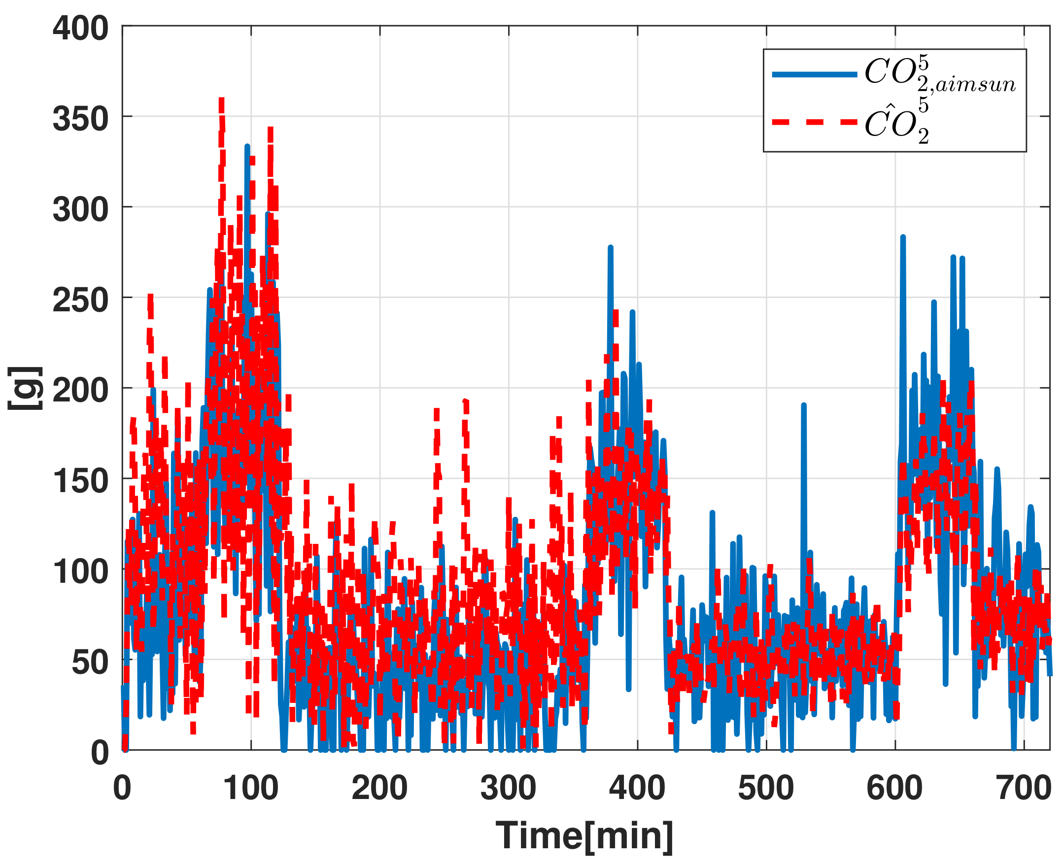
Pollutant Emission Evaluation

The Aimsun Next validation software was used to conduct a preliminary assessment of pollutant emissions caused by the presence of traffic within the considered road network. In particular, to provide a pollutant emissions estimate, the following variables were utilized:

• The vehicle traffic estimate provided by the Luenberger state observer.
• The Aimsun Next “Pollutant Emission” data to reconstruct the information related to carbon dioxide ($C{O}_2$) based on the estimated vehicle traffic.

The obtained results are shown in Figure 14, Figure 15 and Figure 16 where the pollutant emission estimation performance are reported. In particular, these figures report, for the road sectors $R_1$, $R_2$, and $R_4$, a comparison between $C{O}_2$ emissions provided by the “Pollutant Emission” Aimsun Next module (blue line) and the $C{O}_2$ estimate obtained by accounting for the proposed estimation architecture (red dashed line). The outcomes presented indicate that our procedure effectively approximated pollutant emissions in the traffic network. From these initial findings, it is plausible to suggest that the proposed methodology could be a promising solution for the estimation of pollutant emissions in traffic networks.

8. Conclusions

This paper addressed a sensor selection problem for traffic monitoring in road network systems. Using a compartmental network traffic model, the problem was transformed into a mixed-integer nonlinear programming problem. The global minimizer was determined by minimizing the condition number of the observability Gramian while adhering to a budget constraint on the maximum number of sensors. Simulated annealing was employed to find the global minimizer. Numerical simulations validated the approach, comparing favorably with heuristics based on genetic algorithms and exhaustive searches. The proposed approach is simple, yielding a minimal set of sensors with effective observability and state reconstruction performance. Results were used to estimate pollutant emissions in the road network, showing promise but warranting further investigation in future work. In conclusion, we want to emphasize that this study primarily sought to innovate in vehicular traffic estimation by employing a limited set of sensors. Additionally, we aimed to estimate traffic-induced emissions, recognizing that these emissions are influenced by various vehicle attributes, including type and engine specifics. Given the limitations of our current approach in addressing these variables, our ongoing efforts are focused on integrating traffic diversity into our models. This includes the adoption of cutting-edge video processing algorithms for comprehensive traffic classification, promising to elevate the accuracy of our traffic and emissions’ estimations.

References

- Harmon, R.R.; Castro-Leon, E.; Bhide, S. Smart cities and the Internet of Things. In Proceedings of the 2015 Portland International Conference on Management of Engineering and Technology (PICMET), Portland, OR, USA, 2–6 August 2015; pp. 485–494. [Google Scholar] [CrossRef]
- Monzon, A. Smart cities concept and challenges: Bases for the assessment of smart city projects. In Proceedings of the 2015 International Conference on Smart Cities and Green ICT Systems (SMARTGREENS), Lisbon, Portugal, 20–22 May 2015; pp. 1–11. [Google Scholar]
- Kumar, B.; AbuAlhaija, M.; Alqasmi, L.; Dhakhri, M. Smart Cities: A New Age of Digital Insecurity. In Proceedings of the 2020 9th International Conference System Modeling and Advancement in Research Trends (SMART), Moradabad, India, 4–5 December 2020; pp. 267–272. [Google Scholar] [CrossRef]
- Ali, M.; Scandurra, P.; Moretti, F.; Blaso, L. Architecting a big data-driven software architecture for smart street lighting. In Proceedings of the 2023 IEEE 20th International Conference on Software Architecture Companion (ICSA-C), L’Aquila, Italy, 13–17 March 2023; pp. 1–10. [Google Scholar] [CrossRef]
- Manyake, M.K.; Mathaba, T.N.D. An Internet of Things Framework for Control and Monitoring of Smart Public Lighting Systems: A Review. In Proceedings of the 2022 International Conference on Artificial Intelligence, Big Data, Computing and Data Communication Systems (icABCD), Durban, South Africa, 4–5 August 2022; pp. 1–9. [Google Scholar] [CrossRef]
- Casavola, A.; Franzé, G.; Gagliardi, G.; Tedesco, F. Improving Lighting Efficiency for Traffic Road Networks: A Reputation Mechanism Based Approach. IEEE Trans. Control Netw. Syst. 2022, 9, 1743–1753. [Google Scholar] [CrossRef]
- Georges, D. The use of observability and controllability gramians or functions for optimal sensor and actuator location in finite-dimensional systems. In Proceedings of the 1995 34th IEEE Conference on Decision and Control, New Orleans, LA, USA, 13–15 December 1995; Volume 4, pp. 3319–3324. [Google Scholar] [CrossRef]
- Ru, Y.; Hadjicostis, C.N. Optimal sensor selection for structural observability in discrete event systems modeled by Petri Nets. IFAC Proc. Vol. 2007, 40, 223–228. [Google Scholar] [CrossRef]
- Joshi, S.; Boyd, S. Sensor Selection via Convex Optimization. IEEE Trans. Signal Process. 2009, 57, 451–462. [Google Scholar] [CrossRef]
- Hinson, B.T. Observability-Based Guidance and Sensor Placement. Ph.D. Dissertation, University of Washington, Seattle, WA, USA, 2014. Available online: https://digital.lib.washington.edu/researchworks/bitstream/handle/1773/27387/Hinson_washington_0250E_14008.pdf?sequence=1 (accessed on 1 November 2023).
- Lee, B.H.; Deininger, R.A. Optimal locations of monitoring stations in water distribution system. J. Environ. Eng. 1992, 118, 4–16. [Google Scholar] [CrossRef]
- Watson, J.P.; Greenberg, H.J.; Hart, W.E. A multipleobjective analysis of sensor placement optimization in water networks. In Proceedings World Water and Environment Resources; ASCE: New York, NY, USA, 2004. [Google Scholar]
- Ostfeld, A.; Salomons, E. Optimal layout of early warning detection stations for water distribution systems security. J. Water Resour. Plan. Manag. 2004, 130, 377–385. [Google Scholar] [CrossRef]
- Kessler, A.; Ostfeld, A.; Sinai, G. Detecting accidental contaminations in municipal water networks. J. Water Resour. Plan. Manag. 1998, 124, 192–198. [Google Scholar] [CrossRef]
- Kumar, A.; Kansal, M.L.; Arora, G. Discussion of ‘detecting accidental contaminations in municipal water networks’ by A. Kessler, A. Ostfeld, and G. Sinai. J. Water Resour. Plan. Manag. 1999, 125, 308–309. [Google Scholar] [CrossRef]
- Muller, H.H.; Castro, C.A. Genetic algorithm-based phasor measurement unit placement method considering observability and security criteria. IET Gener. Transm. Distrib. 2016, 10, 270–280. [Google Scholar] [CrossRef]
- Yuan, P.; Ai, Q.; Zhao, Y. Research on multi-objective optimal PMU placement based on error analysis theory and improved GASA. Proc. CSEE 2014, 34, 2178–2187. [Google Scholar]
- Prasad, S.; Kumar, D.M.V. Trade-offs in PMU and IED deployment for active distribution state estimation using multi-objective evolutionary algorithm. IEEE Trans. Instrum. Meas. 2018, 67, 1298–1307. [Google Scholar] [CrossRef]
- Chepuri, S.P.; Leus, G. Sensor selection for estimation, filtering, and detection. In Proceedings of the 2014 International Conference on Signal Processing and Communications (SPCOM), Bangalore, India, 22–25 July 2014; pp. 1–5. [Google Scholar] [CrossRef]
- Fu, Y.; Ling, Q.; Tian, Z. Distributed sensor allocation for multi-target tracking in wireless sensor networks. IEEE Trans. Aerosp. Electron. Syst. 2012, 48, 3538–3553. [Google Scholar] [CrossRef]
- Hernandez, M.L.; Kirubarajan, T.; Bar-Shalom, Y. Multisensor resource deployment using Posterior Cramer-Rao bounds. IEEE Trans. Aerosp. Electron. Syst. 2004, 40, 399–416. [Google Scholar] [CrossRef]
- Zhan, P.; Casbeer, D.W.; Swindlehurst, A.L. Adaptive mobile sensor positioning for multi-static target tracking. IEEE Trans. Aerosp. Electron. Syst. 2010, 46, 120–132. [Google Scholar] [CrossRef]
- Gagliardi, G.; Casavola, A.; D’Angelo, V. Traffic Sensors Selection for Complete Link Flow Observability through Simulated Annealing. IFAC-PapersOnLine 2023, 56, 10540–10545. [Google Scholar] [CrossRef]
- Gagliardi, G.; Casavola, A.; D’Angelo, V. Reliable Traffic Sensor Networks Via Fault-Tolerant Sensor Reconciliation Schemes. IFAC-PapersOnLine 2023, 56, 10558–10563. [Google Scholar] [CrossRef]
- Schizas, I.D. Distributed Informative-Sensor Identification via Sparsity-Aware Matrix Decomposition. IEEE Trans. Signal Process. 2013, 61, 4610–4624. [Google Scholar] [CrossRef]
- Varotto, L.; Zampieri, A.; Cenedese, A. Street Sensors Set Selection through Road Network Modeling and Observability Measures. In Proceedings of the 2019 27th Mediterranean Conference on Control and Automation (MED), Akko, Israel, 1–4 July 2019; pp. 392–397. [Google Scholar] [CrossRef]
- Gendreau, M.; Potvin, J.-Y. (Eds.) Handbook of Metaheuristics; International Series in Operations Research & Management Science 146; Springer Science+Business Media, LLC: Berlin/Heidelberg, Germany, 2010. [Google Scholar] [CrossRef]
- Crosson, E.; Harrow, A.W. Simulated Quantum Annealing Can Be Exponentially Faster Than Classical Simulated Annealing. In Proceedings of the 2016 IEEE 57th Annual Symposium on Foundations of Computer Science (FOCS), New Brunswick, NJ, USA, 9–11 October 2016; pp. 714–723. [Google Scholar] [CrossRef]
- Coogan, S.; Arcak, M. A Compartmental Model for Traffic Networks and Its Dynamical Behavior. IEEE Trans. Autom. Control 2015, 60, 2698–2703. [Google Scholar] [CrossRef]
- Walter, G.G.; Contreras, M. Compartmental Modeling with Networks, 1st ed.; Birkhauser Boston, Inc.: Secaucus, NJ, USA, 1998. [Google Scholar]
- Ljung, L. System Identification: Theory for the User, 2nd ed.; Prentice Hall PTR: Lebanon, IN, USA, 1999. [Google Scholar]
- Liepins, G.E.; Hilliard, M.R. Genetic algorithms: Foundations and applications. Ann. Oper. Res. 1989, 21, 31–58. [Google Scholar] [CrossRef]
- Yang, M.D.; Yang, Y.F.; Su, T.C.; Huang, K.S. An Efficient Fitness Function in Genetic Algorithm Classifier for Landuse Recognition on Satellite Images. Sci. World J. 2014, 2014, 264512. [Google Scholar] [CrossRef] [PubMed]
- Tsai, C.-W.; Chiang, M.-C. Handbook of Metaheuristic Algorithms. In From Fundamental Theories to Advanced Applications; Elsevier Inc.: Amsterdam, The Netherlands, 2023. [Google Scholar] [CrossRef]
- Lingber, I. Adaptive simulated annealing (ASA): Lessons learned. Control Cybern. 1996, 25, 33–54. [Google Scholar] [CrossRef]
- Gallelli, V.; Guido, G.; Vitale, A.; Vaiana, R. Effects of calibration process on the simulation of rear-end conflicts at roundabouts. J. Traffic Transp. Eng. (Engl. Ed.) 2019, 6, 175–184. [Google Scholar] [CrossRef]