Analyzing the Impacts of Land Use and Network Features on Passenger Flow Distribution at Urban Rail Stations from a Classification Perspective

Abstract

This study employed big data analytics to investigate the impacts of land use and network features on passenger flow distribution at urban rail stations. The aim was to provide decision support for differentiated operational management strategies for various types of rail stations, thereby achieving refined operation and the sustainable development of urban rail systems. First, this study compared clustering results using different similarity measurement functions within the K-means algorithm framework, selecting the optimal similarity measurement function to construct clustering models. Second, factors influencing passenger flow distribution were selected from land use and network features, forming a feature set that when combined with clustering model results, served as input for the XGBoost model to analyze the relationship between various features and the station passenger flow distribution. The case study showed that (1) the clustering results using a dynamic time-warping distance as the similarity measurement function was optimal; (2) the results of the XGBoost model highlighted commercial services and closeness centrality as the most important factors that affected rail station passenger flow distribution; (3) urban rail stations in Nanjing could be categorized into four types: “strong traffic attraction stations”, “balanced traffic attraction stations”, “suburban strong traffic occurrence stations”, and “distant suburban strong traffic occurrence stations”. Differentiated operational and management strategies were developed for these station types. This paper offers a novel approach for enhancing the operational management of urban rail transit, which not only boosts operational efficiency but also aligns with the goals of sustainable development by promoting resource-efficient transportation solutions.

1. Introduction

In recent years, the global scale of urban rail transit networks has continued to grow, and an increasing number of cities have entered the urban rail transit network operation stage [1]. Wikipedia data indicate that as of December 2023, a total of 215 cities worldwide are operating urban rail transit systems. Among them, 41 cities have constructed 100 or more stations, 75 cities operate three or more rail lines, and 61 cities have urban rail networks exceeding 100 km in size [2]. Especially in China, where urban rail transit is developing rapidly, by the end of 2022, 26 cities had entered the urban rail transit network operation stage. A total of 50 cities are implementing urban rail transit network construction plans, and the total length of the planned construction lines in progress is 6675.57 km. It can be seen that as more new lines are put into operation, more new stations will be put into use [3,4]. Studying the classification of urban rail transit stations based on passenger flow distribution characteristics, as well as analyzing the relationship between passenger flow distribution, land use, and network features, helps to clarify resource allocation strategies for different types of stations. This aids in reducing the operational costs of urban rail transit and achieving refined operation, thereby contributing to the broader goals of sustainable development.

Research indicates a widespread interest in exploring various facets of rail transit station passenger flow characteristics, particularly in China, where the rapid development of rail transit has prompted significant contributions from Chinese scholars in this field. Scholars have extensively investigated the passenger flow features of rail transit stations, examining aspects such as boarding and alighting passenger flows [5,6], peak hours passenger flows [7,8,9,10], and weekday versus weekend passenger flows [11,12]. While discrepancies in research conclusions regarding the influencing factors of urban rail station passenger flow exist, they primarily result from variations in study cases, data sources, and adopted models. However, with advancements in information technology, research data have shifted from conventional survey data to big data, leading to more precise expressions of influencing factor indicators [10,11,13,14,15,16]. In terms of research methodologies, linear regression models have been widely utilized to analyze the relationship between urban rail station passenger flow characteristics and influencing factors [5,6,8,16,17]. To better discern commonalities between stations, many scholars employ clustering algorithms to classify stations before delving into the passenger flow characteristics and influencing factors of different station types [9,18,19].

Although there has been extensive research on the characteristics and influencing factors of urban rail station passenger flow, studies that specifically focused on the distribution of passenger flow at urban rail stations during operational phases are relatively scarce. Furthermore, existing research on station classification often relies on simplistic clustering algorithms, overlooking the significant impact of the clustering quality on subsequent analyses, and many analyses of influencing factors still heavily lean on linear regression models, neglecting potential nonlinear relationships between station passenger flow characteristics and influencing factors, as well as the limitations of linear regression models in addressing classification challenges.

Therefore, this study examined the factors that influenced passenger flow distribution at urban rail transit stations from the perspective of station classification. Understanding these factors is crucial for optimizing station management and enhancing service quality, which, in turn, contributes to the sustainability of urban transportation systems by promoting efficient resource utilization and reducing operational costs. In the station classification module, a time-series clustering approach was utilized to categorize stations, alongside the selection of appropriate similarity measurement functions to enhance the clustering effectiveness. Within the analysis of the influencing factors module, the outstanding classification capabilities and capacity to learn nonlinear relationships of the XGBoost model were leveraged to analyze the impact of factors on station passenger flow distribution. Finally, integrating the results from both modules, the temporal and spatial characteristics of different station types were analyzed to furnish decision-making foundations for the refined operational management of rail transit stations. The remaining part of this paper is organized as follows. A literature review is conducted in Section 2. The research data and method are presented in Section 3. Section 4 details the empirical results and Section 5 provides a discussion. Section 6 presents the conclusions.

2. Literature Review

2.1. Passenger Flow Characteristics

Previous studies investigated station-level passenger flow characteristics from various perspectives: some scholars studied the characteristics of boarding and alighting passenger flows [5,6,15,17,20,21,22]; some scholars intercepted the peak passenger flow at stations during peak hours to study the peak characteristics of passenger flow at urban rail stations [7,8,9,10]; An and Li et al. subdivided daily passenger flow into weekdays and weekends based on whether the main purpose of travel was commuting [7,11,12]; Yang et al. extracted passenger flow data with commuting characteristics from the travel chain and conducted research on it [9]; Yin et al. extracted statistical characteristic values, such as maximum value, kurtosis, skewness, and peak coefficient, from daily passenger flow data to study the characteristics of urban rail station passenger flow [18]; in order to explore more fine-scale features, Wang et al. studied the hourly changes in passenger flow on weekdays and weekends [16]; although there were studies on the passenger flow at urban rail stations from different perspectives, there has been relatively little research on the distribution of passenger flow at urban rail stations. For the networked operation of urban rail transit, it is necessary to grasp the characteristics of passenger flow distribution at different stations to develop refined management strategies and improve the operational management efficiency.

2.2. Influence Factors and Research Data

Early research on the influencing factors of passenger flow at urban rail stations is mainly based on survey and statistical data, for example, built environment factors, such as population, employment, and land use, as well as network factors, such as road networks, bus networks, and rail networks [17,20,23,24]. Research on Seoul metro stations indicates that population, employment, office spaces, and commercial land use are significant factors influencing station passenger flow [20]. Research on Nanjing metro stations revealed that factors such as the length of roads within the pedestrian catchment area, the number of connecting bus routes, park and ride (P&R) spaces, and whether the rail transit station serves as a transfer station also have significant impacts on station passenger flow [24]. The survey and statistical data have the disadvantages of high cost and coarse scale, as they are mainly derived from government statistical data at the administrative district level or travel surveys conducted at the traffic analysis zone (TAZ) level.

With the development of information and communication technology (ICT), big data, especially spatiotemporal data, has been widely utilized in various studies [25], including social media data, OpenStreetMap, points of interest (POIs), and automatic fare collection (AFC) data. OpenStreetMap can provide more accurate data on road traffic infrastructure, allowing for the computation of features such as road lengths within the PCA [10]. POI data have advantages such as easy accessibility and more accurate identification of land-use types [13]. Therefore, in recent research, POI data have been widely used to calculate land use characteristic indicators. However, due to the detailed classification of POI data (for example, Amap categorizes POIs into 19 classes), many scholars perform further processing on POI data to better represent land-use characteristics, select several types of POI data with strong correlation to represent a certain land type [15], or reclassify POI data [10,11].

With the use of big data, further discoveries have been made regarding the factors influencing urban rail station passenger flow. A case study of the Beijing metro system demonstrated that land-use entropy has a significant impact on both boarding and alighting passenger flows [21]. An et al. found that factors such as betweenness centrality, whether a station is a terminal station, and the number of bus stops have a significant impact on urban rail station passenger flow. Simultaneously, the study emphasized that land use is the most crucial factor [11]. Residential, commercial, service, scientific research education area ratio, the number of bus stations, use diversity, the number of entrances at a station, and whether it serves as a transfer station are key factors influencing passenger flow on both weekdays and weekends [7]. Li et al. also demonstrated the importance of bus station density, land-use entropy, and land-use characteristics for station passenger flow [12].

Previous studies fully demonstrated the importance of land use and rail network features on station passenger flow, but some features need further optimization, such as whether rail stations are terminal stations and whether transfer stations often use dummy variables. The degree centrality in complex network indicators can be used for characterization, where the edge connected to the terminal station is 1 and the edge connected to the transfer station is greater than 2. Second, some features are expressed repeatedly. For example, the statistics of traffic facilities in POIs have included the number of bus stops and parking lots.

2.3. Methodology

In terms of research methodologies, the primary approach has been linear regression analysis; in particular, early studies predominantly employed global regression models, like ordinary least squares (OLS) [11,17,24,26,27], Bayesian negative binomial regression (BNBR) [21], and multinomial logistic regression (MLR) [12]. However, global regression models overlooked the spatial heterogeneity of rail stations. Subsequent research often utilized geographically weighted regression (GWR) models to analyze the relationship between the station passenger flow and the influencing factors while considering spatial variations [6,7,28]. To solve the problem that using the same bandwidth for all variables in the GWR model cannot reflect the spatial action scale of different variables, allowing each variable to have its own different spatial smoothing level of multiscale geographically weighted regression (MGWR) makes the fitting results better [8,10]. The geographically and temporally weighted regression (GTWR) model considers both the spatial and temporal heterogeneity in variables. Its application in the case of the Beijing subway demonstrated superior fitting performance compared with the GWR model [16]. Some scholars also improved the explanatory power of GWR models for temporal–spatial heterogeneity by combining them with other models, such as the multimodal logistic (MNL) model [29]. Linear regression models can only capture linear relationships between variables, making it challenging to obtain ideal results for some nonlinear structures. Machine learning models, like XGBoost, effectively address this issue and have achieved favorable results in various publicly available datasets [30]. Liu et al. combined XGBoost regression analysis to study the factors influencing station passenger flow. The results indicate that the XGBoost regression outperformed the OLS model [15].

To better enhance the operational efficiency of urban rail stations based on the factors influencing passenger flow, it is necessary to further analyze the factors for different types of stations. This enables the provision of differentiated operational strategies for different station types. Many scholars started using clustering algorithms to classify rail stations. The commonly used clustering algorithm is K-means [9,18,19], but to avoid the issue of having to predefine the number of clusters, Li et al. employed expectation maximization (EM) clustering for station classification [12]. Previous station classification studies often utilized the Euclidean distance (ED), which lacks a comparison of data shape similarity. However, for time-series clustering, selecting an appropriate similarity measure function can effectively improve the clustering results [31,32]. Therefore, similarity measurement functions, like shape-based distance (SBD) [33], dynamic time warping (DTW) [34,35], and spatiotemporal similarity [36], have gradually been applied to time-series clustering analysis.

In short, the current research faces the following challenges. First, there is still insufficient exploration into the distribution patterns of passenger flow at stations, with previous studies primarily concentrated on statistical characteristics of flows. However, understanding the passenger flow distribution at stations is crucial for effective operational management. Second, previous research demonstrated the significant influence of land use and rail network features on passenger flow at stations. Nonetheless, issues such as redundancy and inaccuracy in feature representation require further refinement to enhance the accuracy and interpretability of models. Third, despite many scholars utilizing big data sources, such as POIs and AFC, for research, data processing methods need refinement to improve the data quality and reliability. Additionally, current research methods primarily rely on the line regression model, neglecting potential nonlinear relationships between station flows and influencing factors, thus limiting model-fitting capabilities. With the rapid expansion of urban rail networks and the increasing number of stations in operation, scholars are increasingly focusing on station classification studies to formulate more targeted management strategies and operational plans. Therefore, constructing composite models and studying the factors influencing passenger flow distribution from a station classification perspective can better elucidate the effects of various factors on the distribution of passenger flows at different stations, thereby enhancing the operational efficiency and service levels at stations.

3. Data and Methodology

3.1. Research Data

3.1.1. Data Source

This study took the urban rail transit system of Nanjing as the research example. The involved data included the following:

• Passenger flow data

Passenger flow data were for Nanjing urban rail stations from 19 September 2022 (Monday) to 25 September 2022 (Sunday). The data covered 11 urban rail lines (excluding trams) and 175 urban rail stations (excluding transfer stations without repetition). A data sample is provided in

Table 1. Example of passenger flow data at Nanjing urban rail station.

Line Name	Station Name	Before 6:00				23:00–24:00
		Entry Count *	Exit Count *	Subtotal	……	Entry Count	Exit Count	Subtotal
Line 1	Zhushan Road	66	6	72		17	133	150
Line 2	Xinjiekou	29	17	46		225	59	284
Line 3	Daxingong	11	3	14		35	19	54
Line 4	Longjiang	73	3	76		2	109	111
……

* Entry (exit) count indicates the number of passengers entering (leaving) the station during this period.

.

2.

POI data

POI data within the 800 m PCA were obtained from the Amap Development Platform. The POI data were categorized into 19 types, such as business and residence, accommodation services, and catering services, totaling 222,147 points of interest. A data sample is presented in

Table 2. Example of POI data.

POI_NAME	POI_ID	WGS84		Type
		Longitude	Latitude
Jiuxinglou Tavern	B0FFL87K4W	118.6224	32.4880	Catering services
Lingfeng Temple	B0FFF3557D	119.0232	31.5590	Tourist attractions
Shengxiang Hotel	B00190COI9	118.9905	31.3962	Lodging services
……

.

3.1.2. Data Preprocessing

The big data processing in this study mainly consisted of two parts: restructuring the entry and exit passenger flow data into time series, standardizing it, and reclassifying the POI data.

• Passenger flow data

According to the requirements of the time-series clustering method for the dataset, the entry and exit passenger flow data of urban rail stations were reconstructed based on “weekday entry—weekday exit—weekend entry—weekend exit.” This restructuring was performed to create a 1-dimensional time series for each rail station, with a length of 76, as shown in Equation (1):

$${\mathrm{X}}_{\mathrm{j}}=\left\{{\mathrm{x}}_{\mathrm{j}}^1,\dots ,{\mathrm{x}}_{\mathrm{j}}^{\mathrm{n}}\right\}$$

(1)

where ${\mathrm{X}}_{\mathrm{j}}$ represents the time series corresponding to the urban rail station j, and ${\mathrm{x}}_{\mathrm{j}}^{\mathrm{n}}$ represents the passenger flow data at the n-th time point for rail station j, where n = 76.

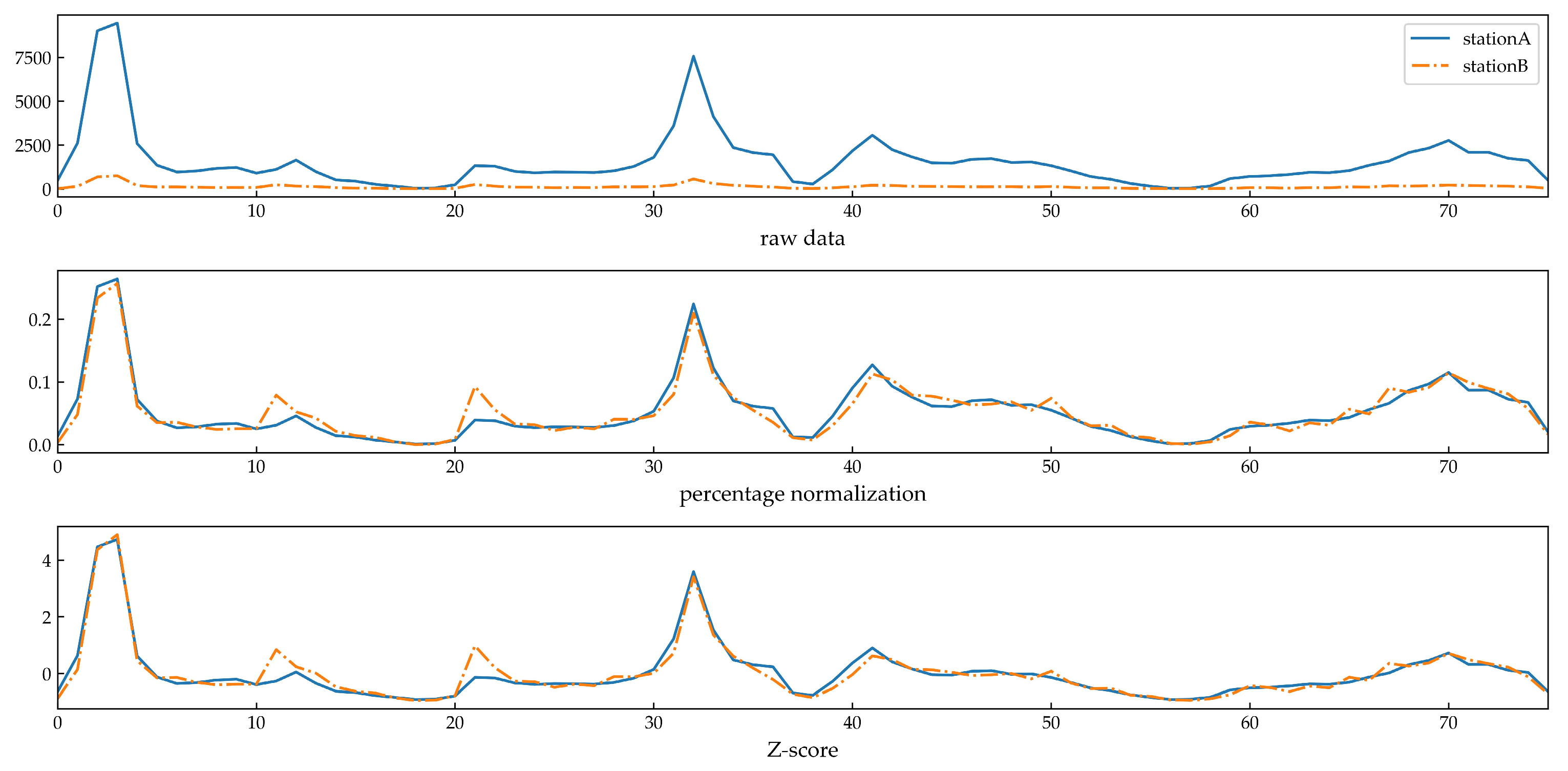
Due to the low passenger flow at some urban rail stations in the initial stages of construction, and to avoid the influence of occasional changes in passenger flow, urban rail stations with a daily passenger flow below 500 people per day were excluded from the dataset. To reduce the impact of random factors, the average entry and exit passenger flow for urban rail stations on weekdays (Monday to Friday) and weekends (Saturday to Sunday) were calculated. This provided the average passenger flow for weekdays and weekends at each station. In the end, 172 valid time series were obtained. Due to significant differences in passenger flow at different urban rail stations, and to mitigate the impact of passenger flow magnitudes on the data waveforms, this study used percentage normalization to standardize the data. The calculation method for the percentage normalization was

$${\mathrm{p}}_{\mathrm{j}}^{\mathrm{i}}=\frac{{\mathrm{x}}_{\mathrm{j}}^{\mathrm{i}}}{{\displaystyle \sum _{\mathrm{i}=1}^{\mathrm{m}}{\mathrm{x}}_{\mathrm{j}}^{\mathrm{i}}}}$$

(2)

where ${\mathrm{p}}_{\mathrm{j}}^{\mathrm{i}}$ represents the proportion of entry (exit) passenger flow during the i-th operational hour to the total entry (exit) passenger flow on the j-th day, ${\mathrm{x}}_{\mathrm{j}}^{\mathrm{i}}$ represents the entry (exit) passenger flow during the i-th operational hour, n represents the total number of operational hours per day for the rail station, and m = 19.

Comparing Figure 1, it can be observed that by removing the influence of the data magnitudes, percentage normalization had the same effect as Z-score normalization. Z-score normalization assigns no practical meaning to the numerical values corresponding to each time point, whereas percentage normalization represents the contribution of each operational hour to the total daily entry (exit) passenger flow. The utilization of percentage normalization preserves the substantive meaning of the data, thereby augmenting the interpretability of the clustering outcomes.

2.

POI data

To comprehensively represent land features, a reclassification of the POI data was performed based on the specific attributes of the land. As delineated in

Table 3. Reclassification of POI data.

New Category Names	Amap Categories	Example Names for POI Data
Commercial services	Car services	Ping An Car Rental
	Car sales	Wuling Baojun Automobile
	Car maintenance	Longteng Automobile Maintenance Service Center
	Motorcycle services	Wuji Moto Service
	Catering services	Bao Family Restaurant
	Retail services	Lao San Convenience Store
	Lifestyle services	China Sports Lottery
	Recreation	Gaochun Cinema and Theater
	Lodging services	Mingfa Jiangwan Hot Spring Hotel
Public services	Healthcare	Gubai Central Health Center
	Government agencies and social organizations	Guihua Village Committee
	Scientific, educational, and cultural services	Xilian Primary School
	Public facilities	Banqiao New Town Emergency Shelter
Tourist attractions	Tourist attractions	Wuxiang Temple Scenic Area
Residential areas	Commercial residential	Wujiang Community
Office spaces	Financial institutions	China Construction Bank
	Companies	Jiangsu Gangxia Group
Transportation services	Transportation facilities	Sichakou Bus Stop
	Roadside infrastructure	Cuiping Mountain Service Area

, the POI data obtained from the Amap development platform were systematically categorized into 6 distinct classes, namely, commercial services, public services, tourist attractions, residential areas, office spaces, and transportation services.

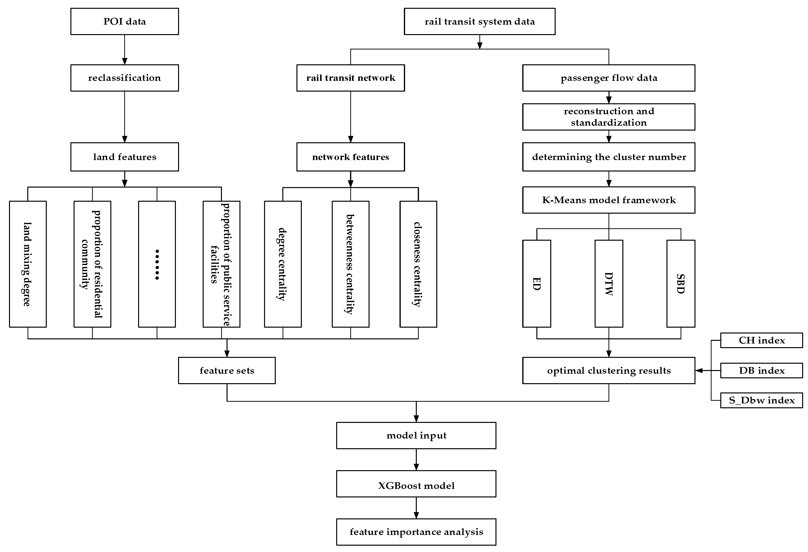
3.2. Research Framework

This study transformed the station entry and exit passenger flow data into time-series data, preprocessed the data using percentage normalization as a standardization method, and then conducted cluster analysis within the framework of the K-means clustering algorithm. The different clustering effects of the ED, DTW, and SBD were compared using evaluation indices: the Calinski–Harabasz (CH) index, Davies–Bouldin (DB) index, and S_Dbw index. The optimal clustering result was selected to label the station categories. This result, along with a feature set comprising 6 land features characterized by POI data and 3 network features calculated from the rail transit network, formed the input for the XGBoost model. The feature importance calculated by the model was then used to analyze the impact of each feature on the station categorization. The research framework is illustrated in Figure 2.

3.3. Methodology

3.3.1. Time-Series Clustering Model

The K-means clustering algorithm is a partitioning-based clustering algorithm that relies on a collection of samples. The fundamental steps are as follows: Step 1 involves randomly selecting k samples as the initial cluster centers. In Step 2, each sample is assigned to the cluster whose center is closest in distance. Following this, Step 3 entails recalculating the center of each cluster by taking the average of its samples. Step 4 iteratively repeats these procedures until the cluster centers no longer change or a predefined number of iterations is reached. In K-means clustering, a similarity measurement function is employed to compute the distance between each data point and the cluster center, facilitating the assignment of data points to the nearest cluster center. This study adopted the ED, DTW, and SBD as the similarity measurement functions in the model.

• ED

When employing the ED to assess the similarity of two time series, it is essential to establish a one-to-one correspondence between the time nodes of the two sequences and compute the distance at each corresponding time node, as illustrated in Figure 3. Due to the inherent limitation of the ED in capturing the similarity of time-series shapes, clustering based on this metric may lead to the grouping of two sequences with substantially different curve shapes but a relatively small ED.

2.

DTW

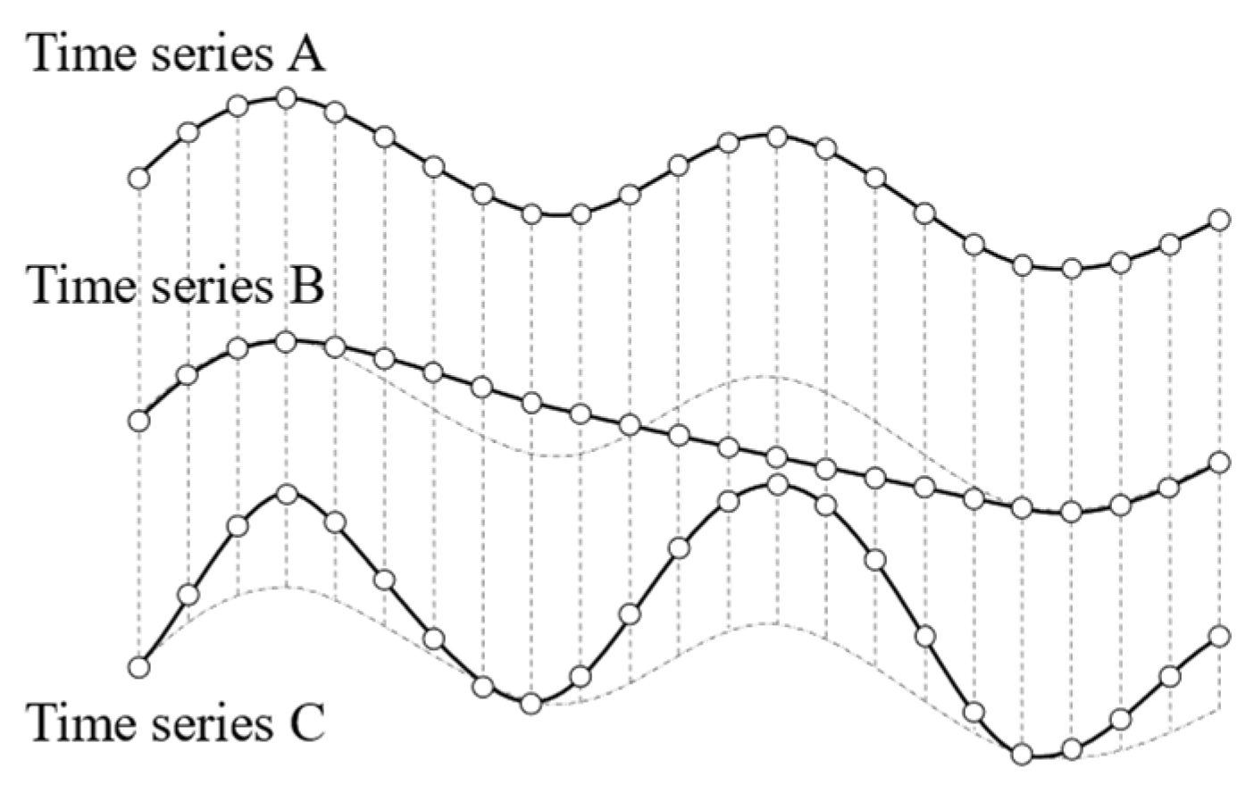
DTW is commonly used to measure the similarity between two time series of different lengths. As shown in Figure 4, when using DTW to measure the similarity between a time series ${\mathrm{A}}_{\mathrm{n}}=({\mathrm{a}}_1,{\mathrm{a}}_2,\dots ,{\mathrm{a}}_{\mathrm{n}})$ of length $n$ and a time series ${\mathrm{B}}_{\mathrm{m}}=({\mathrm{b}}_1,{\mathrm{b}}_2,\dots ,{\mathrm{b}}_{\mathrm{m}})$ of length m, it is necessary to find a continuous correspondence that includes all points in both time series. Initially, a matrix of size n × m is constructed, where the element in the i-th row and j-th column represents the distance ${\mathrm{w}}_{\mathrm{ij}}$ (typically the ED) between the point ${\mathrm{a}}_{\mathrm{i}}$ in time series ${\mathrm{A}}_{\mathrm{n}}$ and the point ${\mathrm{b}}_{\mathrm{j}}$ in time series ${\mathrm{B}}_{\mathrm{m}}$. Then, the objective is to find a monotonically increasing, continuous diagonal path in the matrix with the minimum sum of distances (${\mathrm{D}}_{\mathrm{dtw}}$), which represents the optimal alignment. The calculation formula ${\mathrm{D}}_{\mathrm{dtw}}$ is as follows:

$${\mathrm{D}}_{\mathrm{dtw}}=\frac{{\displaystyle \sum _{\mathrm{k}=1}^{\mathrm{p}}{\mathrm{w}}_{\mathrm{ij}}^{\mathrm{k}}}}{\mathrm{p}}$$

(3)

where ${\mathrm{D}}_{\mathrm{dtw}}$ represents the DTW, ${\mathrm{w}}_{\mathrm{ij}}^{\mathrm{k}}$ represents the matrix element value corresponding to the k-th point in the path, and p represents the number of points in the path.

3.

SBD

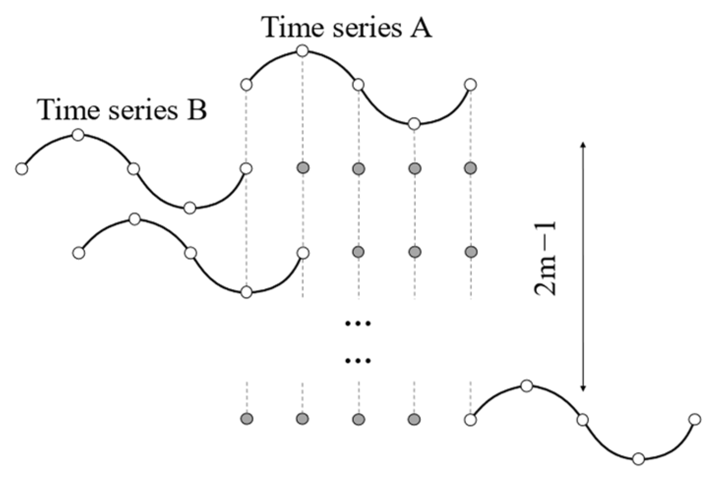
The SBD is an improvement proposed based on the ED, taking into account the characteristic that amplitude scaling and translation do not alter the waveform trend of time series. As shown in Figure 5, when measuring the similarity between time series ${\mathrm{A}}_{\mathrm{m}}=({\mathrm{a}}_1,{\mathrm{a}}_2,\dots ,{\mathrm{a}}_{\mathrm{m}})$ and time series ${\mathrm{B}}_{\mathrm{m}}=({\mathrm{b}}_1,{\mathrm{b}}_2,\dots ,{\mathrm{b}}_{\mathrm{m}})$ using the SBD, ${\mathrm{B}}_{\mathrm{m}}$ is progressively slid over ${\mathrm{A}}_{\mathrm{m}}$ at each time point. The inner product between ${\mathrm{A}}_{\mathrm{m}}$ and ${\mathrm{B}}_{\mathrm{m}}$ is calculated at each step, resulting in a sequence of inner product values denoted as $\begin{array}{cc}{\mathrm{C}}_{\mathsf{\omega }}=({\mathrm{c}}_1,\dots ,{\mathrm{c}}_{\mathsf{\omega }}),& \mathsf{\omega }\in (1,2\mathrm{m}-1)\end{array}$, with a length of 2m − 1. Finally, the maximum value in the sequence ${\mathrm{C}}_{\mathsf{\omega }}$ is selected to calculate the SBD, as expressed in Formula (6):

$${\mathrm{B}}_{\left(\mathrm{s}\right)}=\left\{\begin{array}{cc}(\stackrel{\left|\mathrm{s}\right|}{\overbrace{0,\dots ,0}},{\mathrm{b}}_1,{\mathrm{b}}_2,\dots ,{\mathrm{b}}_{\mathrm{m}-\mathrm{s}}),& \mathrm{s}\ge 0\\ ({\mathrm{b}}_{\mathrm{m}+\mathrm{s}},\dots ,{\mathrm{b}}_{\mathrm{m}-1},{\mathrm{b}}_{\mathrm{m}},\stackrel{\left|\mathrm{s}\right|}{\overbrace{0,\dots ,0}})& \mathrm{s}<0\end{array}\right.$$

(4)

In the equation, ${\mathrm{B}}_{\left(\mathrm{s}\right)}$ represents the time series when sliding with a step size s: s denotes the number of sliding steps from the alignment start point, where a positive value indicates rightward sliding, a negative value indicates leftward sliding, and $\mathrm{s}\in \left[1-\mathrm{m},\mathrm{m}-1\right]$.

$$\mathrm{SBD}=1-\frac{\max ({\mathrm{C}}_{\mathsf{\omega }})}{\sqrt{{\displaystyle \sum _{\mathrm{i}=1}^{\mathrm{m}}{\mathrm{a}}_{\mathrm{i}}^2\times {\displaystyle \sum _{\mathrm{i}=1}^{\mathrm{m}}{\mathrm{b}}_{\mathrm{i}}^2}}}}$$

(5)

In the equation, the SBD is the shape-based distance, ${\mathrm{C}}_{\mathsf{\omega }}$ is the sequence of inner product values, and ${\mathrm{a}}_{\mathrm{i}}$ and represents the i-th elements of the time series ${\mathrm{B}}_{\mathrm{m}}$.

4.

Evaluation Indices

This study utilized the CH index, DB index, and S_Dbw index as evaluation metrics to assess the clustering performance of various time-series clustering models.

The CH index measures the clustering effectiveness by calculating the ratio of the between-cluster covariance to the within-cluster covariance. A higher CH index indicates a better clustering performance, where a smaller within-cluster covariance and larger between-cluster covariance contribute to a higher CH index.

The DB index measures the clustering effectiveness by calculating the ratio of the average distance between two points within a cluster to the distance between the cluster centers. A smaller DB index indicates better clustering performance, with smaller average distances between points within a cluster and larger distances between cluster centers contributing to a smaller DB index.

The S_Dbw index measures the clustering effectiveness by calculating the sum of compactness within clusters and the density between clusters. A smaller S_Dbw index indicates a better clustering performance, and the clustering results are independent of the algorithm used. The equations for calculating the S_Dbw index are as follows:

$${\mathrm{S}}_{\mathrm{S}\_\mathrm{Dbw}}=\mathrm{Scat}+\mathrm{Dens}\_\mathrm{bw}$$

(6)

$$\mathrm{Scat}=\frac{1}{\mathrm{k}}{\displaystyle \sum _{\mathrm{i}=1}^{\mathrm{k}}\frac{{‖\mathsf{\sigma }({\mathrm{A}}_{\mathrm{i}})‖}_2}{{‖\mathsf{\sigma }\left(\mathrm{E}\right)‖}_2}}$$

(7)

$$\mathrm{Dens}\_\mathrm{bw}=\frac{1}{\mathrm{k}(\mathrm{k}-1)}{\displaystyle \sum _{\mathrm{i}=1}^{\mathrm{k}}{\displaystyle \sum _{\mathrm{j}=1,\mathrm{i}\ne \mathrm{j}}^{\mathrm{k}}\frac{\mathrm{density}({\mathrm{c}}_{\mathrm{ij}})}{\max \left(\mathrm{density}\right({\mathrm{c}}_{\mathrm{i}}),\mathrm{density}({\mathrm{c}}_{\mathrm{j}}\left)\right)}}}$$

(8)

$$\left\{\begin{array}{c}\mathrm{stdev}=\frac{1}{\mathrm{k}}\sqrt{{\displaystyle \sum _{\mathrm{i}=1}^{\mathrm{k}}{‖\mathsf{\sigma }({\mathrm{A}}_{\mathrm{i}})‖}_2}}\\ \mathrm{d}(\mathrm{x},{\mathrm{c}}_{\mathrm{i}})={‖\mathrm{x}-{\mathrm{c}}_{\mathrm{i}}‖}_2\\ \mathrm{f}(\mathrm{x},{\mathrm{c}}_{\mathrm{i}})=\left\{\begin{array}{c}0\hspace{1em}\mathrm{d}(\mathrm{x},{\mathrm{c}}_{\mathrm{i}})>\mathrm{stdev}\hfill \\ 1\hspace{1em}\mathrm{d}(\mathrm{x},{\mathrm{c}}_{\mathrm{i}})\le \mathrm{stdev}\hfill \end{array}\right.\\ \mathrm{density}({\mathrm{c}}_{\mathrm{i}})={\displaystyle \sum _{\mathrm{x}\in {\mathrm{A}}_{\mathrm{i}}}\mathrm{f}(\mathrm{x},{\mathrm{c}}_{\mathrm{i}})}\\ \mathrm{density}({\mathrm{c}}_{\mathrm{ij}})={\displaystyle \sum _{\mathrm{x}\in ({\mathrm{A}}_{\mathrm{i}}\cup {\mathrm{A}}_{\mathrm{j}})}\mathrm{f}(\mathrm{x},{\mathrm{c}}_{\mathrm{ij}})}\end{array}\right.$$

(9)

In these equations, ${\mathrm{S}}_{\mathrm{S}\_\mathrm{Dbw}}$ is the S_Dbw index, $\mathrm{Scat}$ is the compactness within clusters, $\mathrm{Dens}\_\mathrm{bw}$ is the density between clusters, k is the number of clusters, ${\mathrm{A}}_{\mathrm{i}}$ is the dataset of cluster i, E is the dataset of samples, ${\mathrm{c}}_{\mathrm{i},\mathrm{j}}$ is the centroid of clusters i and j, and ${\mathrm{c}}_{\mathrm{ij}}$ is the midpoint of the centroids of clusters i and j.

3.3.2. XGBoost Model

This study placed a significant emphasis on feature extraction from both the rail network and station land use. The goal was to construct a comprehensive feature set to delve deeply into the relationship between the passenger flow distribution at urban rail stations and these features. To meet the requirements of supervised learning on the dataset, the urban rail stations underwent labeling using clustering algorithms.

In terms of the network features, three key metrics were selected: degree centrality, betweenness centrality, and closeness centrality. Degree centrality gauges the importance of nodes directly within the network, while betweenness centrality reflects station usage frequency through the shortest path count. Closeness centrality unveils the proximity of nodes to other nodes.

In the realm of land-use features, the focus centers on two crucial elements: the land-mixing degree derived from POI data and the proportional representation of distinct land-use categories. The quantification of the land-mixing degree utilizes information entropy, providing valuable insights into the heterogeneous composition of land use in the vicinity of stations. Additionally, detailing the percentage distribution of diverse land-use types offers a comprehensive overview of the spatial arrangement of various land uses surrounding these stations.

The choice of the XGBoost model for feature analysis was rooted in its exceptional performance with complex datasets and its ability to capture intricate inter-feature relationships. As a gradient-boosting algorithm, XGBoost assembles a robust ensemble model by combining multiple weak learners, making it well-suited for high-dimensional data and nonlinear associations. The introduced regularization terms prevent overfitting, contributing to its outstanding performance on the medium-sized dataset in this study. Furthermore, XGBoost’s built-in feature importance evaluation enhances the understanding of each feature’s impact on model predictions, thereby improving the model interpretability.

4. Results

4.1. Selection of Similarity Measurement Functions

The K-means clustering algorithm required determining the number of clusters beforehand. The silhouette coefficient method was employed to determine the number of clusters. As shown in Figure 6, the silhouette coefficient was relatively ideal when the number of clusters was 4. Therefore, the number of clusters was chosen as 4.

In the analysis of the Nanjing rail system data, evaluation indices for clustering results using various similarity measurement functions were computed. As shown in

Table 4. Result of model.

Indexes	K-Means Algorithm Framework
	DTW	ED	SDB
CH index	64.779	63.981	62.899
DB index	1.446	1.461	1.476
S_Dbw index	0.664	0.681	0.670

, clustering results based on DTW outperformed other similarity measurement functions, exhibiting superior values in the CH index, DB index, and S_Dbw index compared with the ED and SBD. Consequently, the preference was for the K-means clustering model using DTW as the similarity measure function for station clustering in this case data.

4.2. Spatiotemporal Features

4.2.1. Temporal Features

The clustering results, which are illustrated in Figure 7, reveal distinct temporal patterns in passenger flows for the four clusters. Notably, weekdays showed a greater fluctuation in the flow curves compared with weekends. Additionally, variations existed in the temporal distribution of entering and exiting passenger flows.

Cluster 1: On weekdays, the distribution curves of entering and exiting passenger flows exhibited a “balanced” double-peak pattern. The morning peak for entering the passenger flow was from 7:00 to 8:00, and the evening peak was from 17:00 to 18:00. For the exiting passenger flow, the morning peak was from 7:00 to 9:00, and the evening peak was from 18:00 to 19:00. The contribution of each peak’s passenger flow was around 20%. On weekends, there were no distinct peak values in the distribution curves for the entering and exiting passenger flows.

Cluster 2: On weekdays, the distribution curves of the entering and exiting passenger flows showed a “size” double-peak pattern. The morning and evening peaks for the entering and exiting passenger flows were the same as in cluster 1, but compared with cluster 1, the morning peak for the exiting passenger flow and the evening peak for the entering passenger flow had higher peak values. The contribution of the morning peak in the exiting passenger flow was around 25%. On weekends, there were no distinct peak values in the distribution curves for the entering and exiting passenger flows, and compared with cluster 1, there was greater fluctuation in the passenger flows.

Cluster 3: On weekdays, the distribution curves of the entering and exiting passenger flows showed a single-peak pattern. The peak for the entering passenger flow was from 7:00 to 8:00, and the peak for the exiting passenger flow was from 18:00 to 19:00. The contribution of the passenger flow during peak hours was around 25%. On weekends, the distribution curves of the entering and exiting passenger flows showed a skewed peak pattern, similar to weekdays. The entering passenger flow was concentrated in the morning peak, and the exiting passenger flow was concentrated in the evening peak. The contribution of passenger flow during peak hours was around 10%.

Cluster 4: On weekdays, the distribution curves of the entering and exiting passenger flows was somewhat similar to cluster 3, but the peak for the entering passenger flow was from 6:00 to 7:00, 1 h earlier than in cluster 3, and the peak value was lower than in cluster 3. On weekends, the distribution of entering and exiting passenger flows showed a certain double-peak trend, with the passenger flows mainly concentrated in the morning and evening peak periods. The contribution of the passenger flow during peak hours was around 10%.

4.2.2. Spatial Features

According to the information shown in Figure 8, the spatial distribution of the four types of urban rail stations can be observed as follows: The stations in cluster 2 were mainly concentrated in the central area of the rail network, i.e., the core region of the city. The stations in cluster 1, on the other hand, were primarily distributed in the peripheral area of cluster 2. Even when the stations from both cluster 2 and cluster 1 appeared in the outer regions of the rail network, they were still in relatively central parts. The stations in cluster 3 were mainly found in the suburban areas of the city, while the stations in cluster 4 were primarily situated in the outermost regions of the rail network, i.e., the far outskirts of the city. Overall, the four types of stations exhibited a characteristic spatial distribution, gradually transitioning from the city’s core to its outskirts.

4.3. Feature Importance

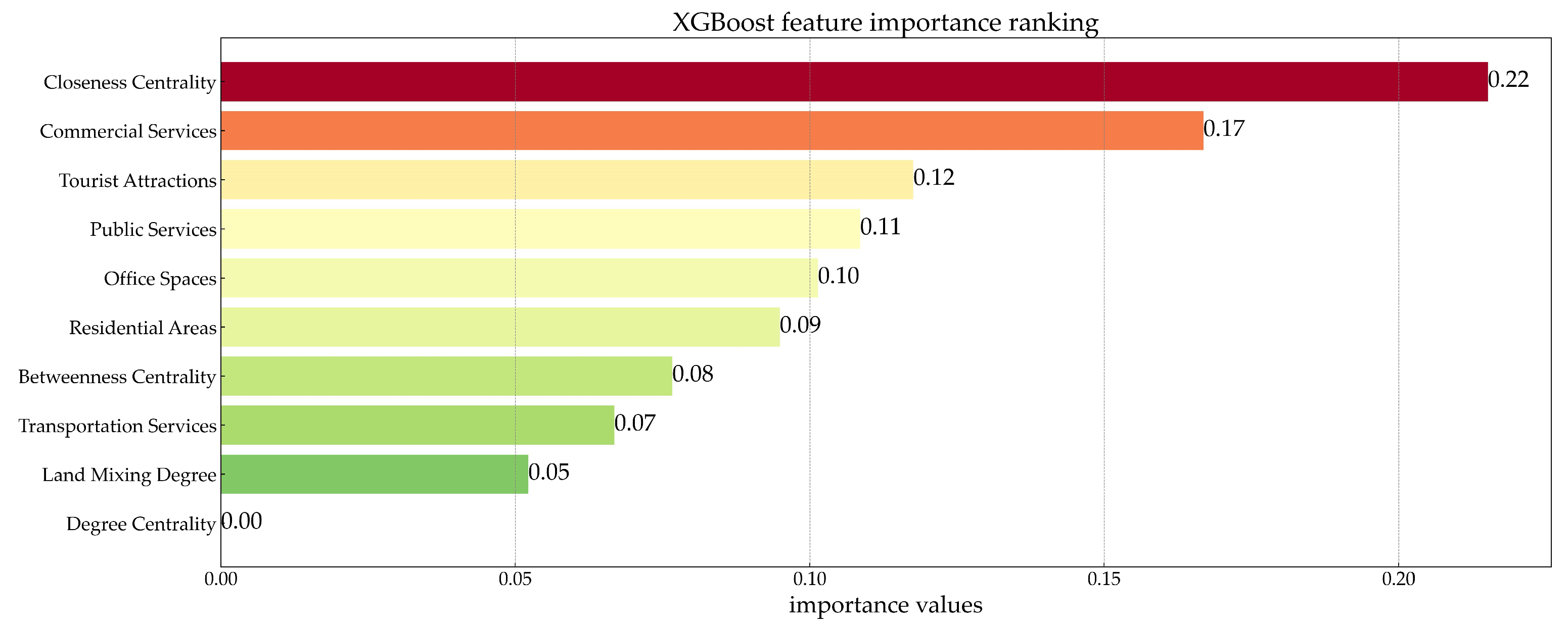
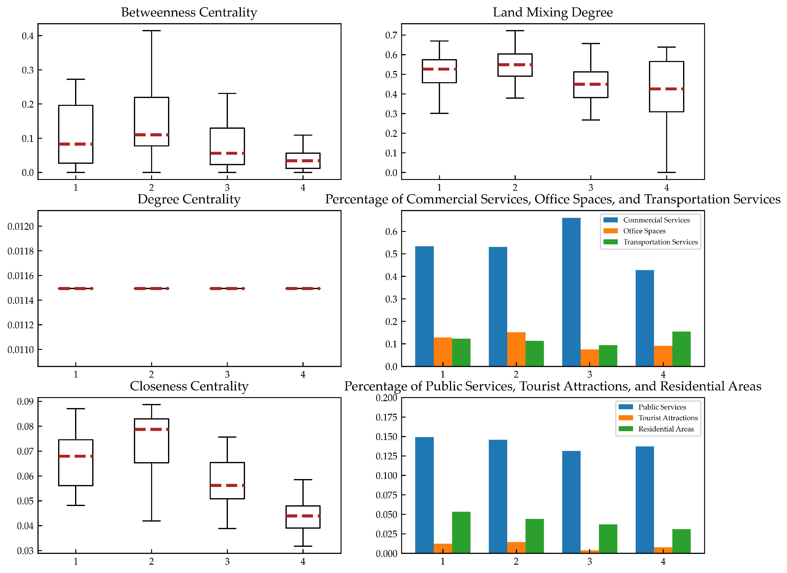
XGBoost model’s feature importance analysis results are shown in Figure 9, and the statistical analysis results of the feature values for each cluster of stations are illustrated in Figure 10. Regarding the network features, the cluster-to-cluster differences were most significant for the feature with the highest importance, which was the closeness centrality. It exhibited a decreasing trend in the order of cluster 2, cluster 1, cluster 3, and cluster 4, indicating that stations in cluster 2 had the shortest average distance to other network stations, followed by cluster 1 and cluster 3, while the stations in cluster 4 had the longest average distance to other network stations. The betweenness centrality with a feature importance of 0.08 showed relatively small inter-cluster differences, following a similar trend to the closeness centrality. The degree centrality had a feature importance of 0, and the average degree centrality was essentially the same for all four cluster types of stations.

In terms of the land features, the inter-cluster variability was highest for the feature with an importance of 0.17, which was the proportion of commercial services. The stations in cluster 3 had the highest average proportion of commercial services, followed by cluster 1 and cluster 2, while the stations in cluster 4 had the lowest average proportion of commercial services. The features with an importance around 0.1, such as the proportions of tourist attractions, public services, office spaces, and residential areas, exhibited relatively large inter-cluster differences. The stations in cluster 2 had the highest proportions of tourist attractions and office spaces, while the stations in cluster 1 had the highest proportions of public services and residential areas. The features of the transportation service proportion and land-mixing degree had a lower importance, and their inter-cluster differences were also smaller. The stations in cluster 4 had the highest transportation service proportion, and the stations in clusters 1 and 2 had higher average land-mixing degrees.

The statistical analysis of different cluster features validated the rationality of the XGBoost model feature importance analysis and provided explanations for the impact of each feature on the station classification. In terms of the network features, the importance of the closeness centrality was the highest, indicating its significant influence on the station classification. The trend of closeness centrality variations for the four clusters of stations was also validated in the spatiotemporal characteristics of stations. The stations in cluster 2, which had the highest closeness centrality, were mainly located in the core area of the rail network, while the stations in cluster 4, which had the lowest closeness centrality, were situated in the outermost regions. Additionally, their maximum average distance to other stations explained why the peak entry of this cluster occurred one hour earlier on weekdays compared with the other clusters. The betweenness centrality had a lower importance, with a variation pattern similar to the closeness centrality, but with smaller inter-cluster differences. The degree centrality had an importance of 0, indicating that whether a rail station was a transfer station did not affect the station classification.

In terms of the land-use features, various features had a certain impact on the station classification: the stations in cluster 2 and cluster 1 had the highest proportions of office services and public services, which explained why these two types of stations exhibited peaks in the morning outbound passenger flow and evening inbound passenger flow. The double-peak trend in the weekend passenger flow for stations in cluster 4 may have been related to their lowest proportion of commercial services. However, unlike the network features, the relationships between the land-use features were more complex, requiring further in-depth research into their impact on the classification of stations. Moreover, due to the lack of consideration for area in the POI data, the proportion of the POI data for a certain land-use attribute may not necessarily reflect the true land-use proportion. For example, the stations in cluster 4 and cluster 3 were located in the outskirts where land prices were relatively lower than in the core area. The same type of POI in the outskirts could occupy a larger area compared with the core area. Perhaps this was why the proportion of residential areas was lower for the stations in cluster 3 and cluster 4, but the peak values during the weekday morning rush hour were higher compared with the stations in cluster 2 and cluster 1.

5. Discussion

Through the analysis of the clustering results, it was observed that different types of urban rail stations exhibited variations in passenger flow distribution characteristics. Additionally, urban rail stations of the same type showed differences in passenger flow distribution patterns on weekdays and weekends. Due to the diverse network and land-use characteristics of urban rail stations, the passenger flow presented distinct distribution features. Essentially, these differences arose from variations in urban spatial layout and land development intensity, leading to the phenomenon of separation between work and residence. Therefore, the urban rail stations were classified into the following four categories:

“High traffic attraction stations” (cluster 2): This type of rail station was mainly located in the core area of the city, surrounded by mature land development and a significant number of office spaces. It had a certain volume of traffic and high traffic attraction. The weekday passenger flow distribution exhibited a “dual peak” characteristic, with significant peaks in the morning and evening rush hours. Due to the high mix of land use around the urban rail station, the overall passenger flow on weekends was relatively stable. Operational strategies for these stations should prioritize efficient passenger flow management during peak hours. In the morning, efforts should focus on streamlining exit routes from the station, while in the evening, entrance facilitation should be emphasized. Given the weekend stability, a consistent but adaptable management resource allocation is necessary to cater to varying demands. Incorporating real-time data analytics can optimize resource distribution, ensuring swift adjustments to passenger flow changes. Additionally, enhancing station accessibility and connectivity with surrounding areas will further improve the passenger experience and station efficiency.

“Balanced station” (cluster 1): This type of urban rail station was predominantly situated in the peripheral regions surrounding the city’s core area. The land development exhibited a certain level of maturity, featuring both office spaces and residential areas. These urban rail stations demonstrated a balanced traffic attraction and occurrence volume. On weekdays, their passenger flow distribution displayed “balanced” bimodal characteristics, while remaining relatively stable during holidays. Management strategies should equally distribute focus between morning and evening peaks by ensuring resource availability that matched the balanced passenger flow. The introduction of flexible staffing and dynamic signage can help to manage the fluctuation in passenger numbers. During weekends, maintaining a steady level of operational management will accommodate the consistent traffic, with special attention to facilitating community events or leisure activities that might influence station use.

“Suburban strong traffic occurrence stations” (cluster 3): This type of urban rail station was mainly located in the suburbs of the city, with the surrounding land primarily consisting of residential areas and supporting commercial facilities. There were fewer office spaces compared with the first two types of stations, but the occurrence of traffic was higher. The weekday passenger flow distribution exhibited a single-peak characteristic. Although there were numerous supporting commercial facilities, the absence of tourist attractions resulted in a more skewed distribution of passenger flow on weekends. For such stations, we can learn from the resource allocation strategy of road traffic for tidal traffic flow and provide more entering service facilities in the morning peaks on weekdays and more exiting service facilities in the evening peaks. At the same time, we should also strengthen the development of plots around the stations; increase the office spaces, tourist attractions, and commercial services; improve the traffic attraction ability; and lift the operational efficiency of the stations.

“Distant suburban strong traffic occurrence stations” (cluster 4): Predominantly located in the city’s outskirts, these stations were surrounded by residential land and bolstered by nearby commercial facilities. Despite having fewer office spaces, they witnessed higher traffic occurrences. On weekdays, the passenger flow distribution displayed a single-peak characteristic. Compared with the “suburban strong traffic occurrence stations”, the more distant location and longer commuting distances led to an earlier morning peak. This station type exhibited the lowest average land-mixing degree, lacking nearby commercial and tourist attractions, resulting in a somewhat dual-peak trend in passenger flow on weekends. Such stations need to pay attention to the early arrival in the morning peak when allocating operational and management resources. The challenge of lower land-mixing degrees and the lack of commercial and tourist attractions necessitates a focused strategy on community and commercial development to stimulate weekend and off-peak usage. Initiatives could include establishing park-and-ride facilities, enhancing connectivity with local transit options, and promoting the station area as a destination through the development of leisure and retail complexes.

The differences in the characteristics of passenger flow changes between weekdays and weekends were mainly due to the different purposes of passenger travel on these days. On weekdays, the peak passenger flows for various types of stations were mostly in the morning and evening rush hours, with the morning peak higher than the evening peak. This was because the primary purpose of weekday passenger travel was commuting, and the commuting times to work were relatively fixed, while the times for returning home were more dispersed. On weekends, there were no significant features in the changes in the passenger flow at stations. This was because the primary purpose of weekend passenger travel was leisure and entertainment, and the travel times were more flexible. However, due to the different rail networks and land-use characteristics of various station types, there were variations in the passenger flow changes on weekends. Therefore, when allocating resources for station operation management, it is necessary to select different resource allocation strategies according to the passenger flow distribution of rail stations, to realize the efficient utilization of rail station resources and the sustainable development of rail transit.

6. Conclusions

This study was based on the AFC data of the Nanjing urban rail system, which were turned into time-series data. This study then utilized the K-means clustering algorithm for cluster analysis and employed the XGBoost model to analyze the feature importance. The main conclusions of this study are as follows:

First, this study conducted a comparative analysis of clustering results using different similarity measurement functions within the K-means framework. The results demonstrate that selecting an appropriate similarity measure function was crucial for enhancing the clustering performance. Specifically, when applied to the AFC data of the Nanjing Metro system, the DTW method emerged as the most suitable for this dataset. This was evidenced by its superior performance in terms of the CH index, DB index, and S_Dbw index. These metrics not only evaluated the quality of clustering but also indicate that the time series extracted from AFC data were well-suited for clustering analysis, with the DTW method yielding more optimal results.

Second, this study delved into station features from the dual perspectives of rail network and land use, resulting in the construction of a comprehensive feature set. By integrating the classification results of the clustering model, a feature analysis was conducted using the XGBoost model. This analytical approach facilitated a systematic evaluation of the importance of each feature, enabling a clear understanding of its impact on station classification. In comparison with other studies, the proportion of commercial services was also identified as a significant factor affecting station classification. However, with the inclusion of network feature analysis, this study uncovered a more critical feature, closeness centrality, which had a greater impact on the passenger flow distribution at the stations. Furthermore, the importance score of the degree centrality being zero indicated that being a transfer or terminal station was not a significant factor that influenced the distribution of passenger flow at urban rail stations. This finding provided a deeper insight into the relationship between these features and the distribution patterns of passenger flow at the stations, highlighting how specific characteristics influenced station categorization and passenger flow distribution.

Finally, the analysis of the instance results, as supported by comprehensive AFC data and feature analysis derived from POI and rail network data, reveals that the 171 urban rail stations could be classified into four distinct categories based on the distribution characteristics of the passenger flow entering and exiting the stations. These categories were “high traffic attraction stations”, which were characterized by a high volume of incoming and outgoing passengers and located in the city’s core area with mature land development; “balance stations”, where the incoming and outgoing passenger flows were relatively balanced and were typically situated in the peripheral regions surrounding the city’s core; “suburban strong traffic occurrence stations”, which were predominantly located in suburban areas with a strong influx of passengers, featuring residential areas and supporting commercial facilities; and “distant suburban strong traffic occurrence stations”, which were further away from the city center and exhibited a significant concentration of passenger traffic and primarily surrounded by residential land. The classification was validated by the features calculated from the POI and rail network data, demonstrating the rationality of this categorization. Based on the unique passenger flow distribution patterns observed in each category, targeted operational management strategies were proposed to address the specific needs and challenges of each station type, thereby contributing to the efficient utilization of rail station resources and the sustainable development of rail transit.

The contribution of this study is to enhance the clustering effect of urban rail stations by selecting appropriate similarity measurement functions and to analyze the influencing factors of station passenger flow distribution in terms of both land use and network features. Leveraging big data, this study employed time-series clustering algorithms and the XGBoost model to provide a comprehensive understanding of how these factors impacted the passenger flow distribution. This research offers targeted operational and management strategies based on the distinct characteristics of station passenger flow distribution, thereby contributing to the optimization of urban rail systems. By enhancing the efficiency and reducing resource waste, these strategies support the sustainable development of urban transportation networks.

In this study, POI data were mainly used, but there was a lack of consideration for land area. At the same time, only rail-network-related features were selected for the influencing factors of network features, and there were no road-network-related indicators, such as the number of intersections and road length, which can be considered in subsequent research.

References

- Han, B.M.; Xi, Z.; Sun, Y.J.; Lu, F.; Niu, S.Q.; Wang, C.X.; Xu, K.L.; Yao, Y.F. Statistical Analysis of Urban Rail Transit Operation in the World in 2022: A Review. Urban Rapid Rail Transit 2023, 36, 1–8. [Google Scholar]
- List of Metro Systems. Available online: https://en.wikipedia.org/wiki/List_of_metro_systems (accessed on 20 January 2024).
- China Urban Rail Transit 2022 Annual Statistical and Analysis Report. Available online: https://www.camet.org.cn/tjxx/11944 (accessed on 22 January 2024).
- Mao, B.H.; Zhang, Z.H.; Chen, Z.J.; Jia, W.Z.; Ho, T.K. A Review on Operational Technologies of Urban Rail Transit Networks. J. Transp. Syst. Eng. Inf. Technol. 2017, 17, 155–163. [Google Scholar] [CrossRef]
- Wang, J.P.; Zhao, M.; Ai, T.; Wang, Q.S.; Liu, Y.F. Revealing the Influence of the Fine-Scale Built Environment on Urban Rail Ridership with a Semiparametric GWPR Model. ISPRS Int. J. Geo-Inf. 2023, 12, 17. [Google Scholar] [CrossRef]
- Zhu, Z.J.; Zhang, Y.; Qiu, S.C.; Zhao, Y.P.; Ma, J.X.; He, Z.P. Ridership Prediction of Urban Rail Transit Stations Based on AFC and POI Data. J. Transp. Eng. Part A-Syst. 2023, 149, 7. [Google Scholar] [CrossRef]
- Li, S.Y.; Lyu, D.J.; Huang, G.P.; Zhang, X.H.; Gao, F.; Chen, Y.T.; Liu, X.P. Spatially varying impacts of built environment factors on rail transit ridership at station level: A case study in Guangzhou, China. J. Transp. Geogr. 2020, 82, 102631. [Google Scholar] [CrossRef]
- Gao, D.H.; Xu, Q.; Chen, P.W.; Hu, J.J.; Zhu, Y.T. Spatial Characteristics of Urban Rail Transit Passenger Flows and Fine-scale Built Environment. J. Transp. Syst. Eng. Inf. Technol. 2021, 21, 25–32. [Google Scholar] [CrossRef]
- Yang, J.; Wu, K.; Zhang, H.L.; Dai, S.X.; Wang, Y.L. Classification of Subway Stations Based on Land Use and Passenger Flow Characteristics. J. Transp. Syst. Eng. Inf. Technol. 2021, 21, 228–234. [Google Scholar] [CrossRef]
- Ma, Z.l.; Yang, X.; Hu, D.W.; Tan, X.W. Influence degree analysis of ridership characteristics at urban rail transit stations. J. Tsinghua Univ. 2023, 63, 1428–1439. [Google Scholar] [CrossRef]
- An, D.D.; Tong, X.; Liu, K.; Chan, E.H.W. Understanding the impact of built environment on metro ridership using open source in Shanghai. Cities 2019, 93, 177–187. [Google Scholar] [CrossRef]
- Li, Q.J.; Peng, J.D.; Yang, H. Research on Relationship Analysis between Passenger Flow Characteristics of Rail Transit Stations and Built Environment of Different Station Areas in Wuhan. J. Geo-Inf. Sci. 2021, 23, 1246–1258. [Google Scholar] [CrossRef]
- Sun, L.S.; Wang, S.W.; Yao, L.Y.; Rong, J.; Ma, J.M. Estimation of transit ridership based on spatial analysis and precise land use data. Transp. Lett. 2016, 8, 140–147. [Google Scholar] [CrossRef]
- Martí, P.; Serrano-Estrada, L.; Nolasco-Cirugeda, A. Social Media data: Challenges, opportunities and limitations in urban studies. Comput. Environ. Urban Syst. 2019, 74, 161–174. [Google Scholar] [CrossRef]
- Liu, X.; Chen, X.H.; Tian, M.S. Effects of Built Environment on Metro Ridership Considering Stage of Growth. J. Transp. Syst. Eng. Inf. Technol. 2023, 23, 121–127. [Google Scholar] [CrossRef]
- Wang, J.; Wan, F.; Dong, C.J.; Yin, C.Y.; Chen, X.Y. Spatiotemporal effects of built environment factors on varying rail transit station ridership patterns. J. Transp. Geogr. 2023, 109, 15. [Google Scholar] [CrossRef]
- Liu, C.; Erdogan, S.; Ma, T.; Ducca, F.W. How to Increase Rail Ridership in Maryland: Direct Ridership Models for Policy Guidance. J. Urban Plan. Dev. 2016, 142, 04016017. [Google Scholar] [CrossRef]
- Yin, Q.; Meng, B.; Zhang, L.Y. Classification of subway stations in Beijing based on passenger flow characteristics. Prog. Geogr. 2016, 35, 9. [Google Scholar]
- Jiang, Y.S.; Yu, G.S.; Hu, L.; Li, Y. Refined Classification of Urban Rail Transit Stations Based on Clustered Station’s Passenger Traffic Flow Features. J. Transp. Syst. Eng. Inf. Technol. 2022, 22, 106–112. [Google Scholar] [CrossRef]
- Sohn, K.; Shim, H. Factors generating boardings at metro stations in the Seoul metropolitan area. Cities 2010, 27, 358–368. [Google Scholar] [CrossRef]
- Zhu, Y.D.; Chen, F.; Wang, Z.J.; Deng, J. Spatio-temporal analysis of rail station ridership determinants in the built environment. Transportation 2018, 46, 2269–2289. [Google Scholar] [CrossRef]
- Pang, L.; Ren, L.J.; Zhang, Z.H.; Yun, Y.X. Metro Station Classification Based on Boarding and Alighting Passenger Flows and Ridership Impact Factors. J. Transp. Syst. Eng. Inf. Technol. 2023, 23, 184–193. [Google Scholar] [CrossRef]
- Cervero, R. Linking urban transport and land use in developing countries. J. Transp. Land Use 2013, 6, 7–24. [Google Scholar] [CrossRef]
- Zhao, J.B.; Deng, W.; Song, Y.; Zhu, Y.R. What influences Metro station ridership in China? Insights from Nanjing. Cities 2013, 35, 114–124. [Google Scholar] [CrossRef]
- Xiao, G.N.; Chen, L.; Chen, X.Q.; Jiang, C.M.; Ni, A.N.; Zhang, C.Q.; Zong, F. A hybrid visualization model for knowledge mapping: Scientometrics, SAOM, and SAO. IEEE Trans. Intell. Transp. Syst. 2023, 25, 2208–2221. [Google Scholar] [CrossRef]
- Kuby, M.; Barranda, A.; Upchurch, C. Factors influencing light-rail station boardings in the United States. Transp. Res. Part A-Policy Pract. 2004, 38, 223–247. [Google Scholar] [CrossRef]
- Sung, H.; Oh, J.T. Transit-oriented development in a high-density city: Identifying its association with transit ridership in Seoul, Korea. Cities 2011, 28, 70–82. [Google Scholar] [CrossRef]
- Cardozo, O.D.; García-Palomares, J.C.; Gutiérrez, J. Application of geographically weighted regression to the direct forecasting of transit ridership at station-level. Appl. Geogr. 2012, 34, 548–558. [Google Scholar] [CrossRef]
- Yue, Y.F.; Chen, J.J.; Feng, T.; Ma, X.W.; Wang, W.; Bai, H. Classification and determinants of high-speed rail stations using multi-source data: A case study in Jiangsu Province, China. Sustain. Cities Soc. 2023, 96, 104640. [Google Scholar] [CrossRef]
- Chen, T.Q.; Guestrin, C. Xgboost: A scalable tree boosting system. In Proceedings of the 22nd ACM SIGKDD International Conference on Knowledge Discovery and Data Mining, San Francisco, CA, USA, 13–17 August 2016; pp. 785–794. [Google Scholar]
- Li, H.L.; Jia, R.Y.; Tan, G.Y. Fuzzy Classification for Time Series Data Based on K-Shape. J. Univ. Electron. Sci. Technol. China 2021, 50, 899–906. [Google Scholar] [CrossRef]
- Li, H.L.; Zhang, L.P. Summary of Clustering Research in Time Series Data Mining. J. Univ. Electron. Sci. Technol. China 2022, 51, 416–424. [Google Scholar]
- Paparrizos, J.; Gravano, L. k-shape: Efficient and accurate clustering of time series. In Proceedings of the 2015 ACM SIGMOD International Conference on Management of Data, Melbourne, VIC, Australia, 31 May–4 June 2015; pp. 1855–1870. [Google Scholar]
- Nagy, V.; Balázs, H. Hidden content of passenger data in public transport. Procedia Comput. Sci. 2017, 109, 506–512. [Google Scholar] [CrossRef]
- Nagy, V.; Horváth, B.; Horváth, R. Land-use zone estimation in public transport planning with data mining. Transp. Res. Procedia 2017, 27, 1050–1057. [Google Scholar] [CrossRef]
- Jiao, H.Z.; Huang, S.B.; Zhou, Y. Understanding the land use function of station areas based on spatiotemporal similarity in rail transit ridership: A case study in Shanghai, China. J. Transp. Geogr. 2023, 109, 103568. [Google Scholar] [CrossRef]