Landscape Evaluation for Restoration Planning on the Okanogan-Wenatchee National Forest, USA

Hessburg, Paul F.; Reynolds, Keith M.; Salter, R. Brion; Dickinson, James D.; Gaines, William L.; Harrod, Richy J.

doi:10.3390/su5030805

Open AccessArticle

Landscape Evaluation for Restoration Planning on the Okanogan-Wenatchee National Forest, USA

¹

USDA Forest Service, Pacific Northwest Research Station, Forestry Sciences Laboratory, 1133 North Western Ave., Wenatchee, WA 98801, USA

²

USDA Forest Service, Pacific Northwest Research Station, Forestry Sciences Laboratory, 3200 SW Jefferson Way, Corvallis, OR 97331, USA

³

USDA Forest Service, Okanogan-Wenatchee National Forest, Wenatchee, WA 98801, USA

^*

Author to whom correspondence should be addressed.

Sustainability 2013, 5(3), 805-840; https://doi.org/10.3390/su5030805

Submission received: 21 November 2012 / Revised: 5 February 2013 / Accepted: 8 February 2013 / Published: 25 February 2013

(This article belongs to the Special Issue Terrestrial Ecosystem Restoration)

Download

Browse Figures

Versions Notes

Abstract

:

Land managers in the western US are beginning to understand that early 20th century forests displayed complex patterns of composition and structure at several different spatial scales, that there was interplay between patterns and processes within and across scales, and that these conditions have been radically altered by management. Further, they know that restoring integrity (see Definition of Terms) of these conditions has broad implications for the future sustainability (see Definition of Terms) of native species, ecosystem services, and ecological processes. Many are looking for methods to restore (see Definition of Terms) more natural landscape patterns of habitats and more naturally functioning disturbance regimes; all in the context of a warming climate. Attention is turning to evaluating whole landscapes at local and regional scales, deciphering recent changes in trajectories, and formulating landscape prescriptions that can restore ecological functionality and improve landscape resilience (see Definition of Terms). The business of landscape evaluation and developing landscape prescriptions is inherently complex, but with the advent of decision support systems, software applications are now available to conduct and document these evaluations. Here, we review several published landscape evaluation and planning applications designed with the Ecosystem Management Decision Support (EMDS) software, and present an evaluation we developed in support of a landscape restoration project. We discuss the goals and design of the project, its methods and utilities, what worked well, what could be improved and related research opportunities. For readability and compactness, fine and broad-scale landscape evaluations that could be a part of multi-scale restoration planning, are not further developed here.

Keywords:

wildland fire; insect outbreaks; sustainability; landscape restoration; landscape planning; EMDS system; climate change; ecological patterns; ecological processes

List of Acronyms

AHP	Analytic Hierarchy Process
CDP	Criterium Decision Plus
CT x SC	Combined cover type and structural class feature
DEM	Digital Elevation Model
DSS	Decision Support System
EMDS	Ecosystem Management Decision Support (system)
ESR	Ecological Subregion
FRV	Future Range of Variation
LSOF	Late-Successional Old Forest
NRV	Natural range of Variation
PLTA	Potential Landscape Treatment Area
PVG x CT x SC	Combined Potential Vegetation Type, Cover Type, and Structural Class Feature
RCF	Risk of Crown Fire
ROS	Rate of Spread
RV	Reference Variation
SMART	Simple Multi-Attribute Rating Technique
SPOW	Spotted owl
WSBW	Western Spruce Budworm

Definition of Terms

Integrity	A landscape has integrity when its ecosystems are fully functional, with all of their biotic and abiotic processes intact.
Sustainability	Conditions that support native species, ecosystem services, and ecological processes are sustainable when influences on them have not resulted in significant depletion or permanent damage.
Restoration	The applied practice of renewing degraded and damaged landscapes, habitats and ecosystems with active human intervention.
Resilience	The inherent capacity of a landscape or ecosystem to maintain its basic structure and organization in the face of disturbances, both common and rare.

Summary

Over the last several centuries, human settlement, development and management have altered the ecological patterns and processes of forested landscapes across the US such that nearly all ecosystems have been touched by at least one of these influences. For example, wildfire suppression and exclusion via road and rail construction and domestic livestock grazing have even altered the structure and processes of wilderness and roadless areas. In the U.S. Inland Northwest, these influences occurred in the late 19th and 20th centuries. Today, few forests on these vast public lands fully support their native flora and fauna, and large and severe wildfires and insect outbreaks are relatively common occurrences. In response, there is public mistrust of foresters and land managers and a succession of environmental laws constraining forest management.

A fair litmus test for the level of mistrust can be seen in the hundreds of legal appeals of Forest- and project-level management plans on public lands, and in the seemingly endless supply of lawsuits brought to bear on timber sales (also known as vegetation management projects) by conservation and forest products organizations, embattled by decades of struggle. Conservation organizations desire less management overall and more environmentally friendly management where occurring, while forest products organizations call for larger timber harvests and more predictable and non-declining timber supplies to sawmills and local economies. Both sides represent valuable stakeholder perspectives, but blending them has proven difficult. In short, there is little shared insight as to methods or philosophies that could guide landscape restoration and maintenance in a manner that both cooperates with native ecosystem structure and function and maintains local economies.

Toward a shared vision and goals, stakeholders in eastern Washington State are beginning to develop a common language, understanding, and appreciation of the consequences of past forest management, and future trajectories of forests with climatic warming. A shared view of ecologically and socially desirable forest restoration goals and methods may be slowly emerging. Here, we discuss recent progress to (1) develop a decision support tool, that (2) evaluates key landscape pattern and process departures from historical and climate change reference conditions, and (3) enables managers and others to evaluate landscape restoration prescriptions as alternative scenarios, before they are implemented. The tool gives managers, and their collaborators, the ability to jointly and graphically consider key changes in landscape patterns, processes, and interactions, and puts these changes in the context of current and future climatic conditions. It also enables formulation and comparison of a variety of landscape prescriptions that can restore, to varying degrees, ecological patterns and functionality, in the context of human social values and preferences.

1. Introduction

1.1. Background

Subsistence agriculture, hunting, and intentional burning activities dominated early Native American management of the Holocene North American landscape. These activities enabled colonization of the continent and cultural development over thousands of years, but not without attendant landscape impacts [1,2,3,4,5]. Native American burning created new and expanded existing herblands, meadows, and open wooded expanses, enhancing harvest of edible plants, nuts, and berries. It also increased sighting distances in the event of sneak-attacks by marauding tribes, and improved forage for wild ungulates, which enhanced hunting both near and away from encampments. Burning along major travel routes improved food supplies and increased ease and safety of travel, but it lacked direct spatial controls on burned area or fire effects, and burns often travelled further and killed more forest than intended. Nonetheless, Native Americans were the first fire managers, and their use of intentionally lighted fires greatly aided their culture and lifestyle.

In the mid-19th century, settlement and management of the Great Plains, and the Pacific, Rocky Mountain, and Intermountain West by Euro-American settlers greatly accelerated with the discovery of lush and productive prairies on the plains and in the intermountain valleys, rich gold and silver ore deposits, and abundant acres for homesteading [1,3,6,7,8,9,10]. With settlement, came land clearing and expansion of agriculture, timber harvesting, and early attempts at wildfire suppression, which were highly effective after the 10 a.m. rule was enacted as federal policy between 1934 and 1935 [1,11]. This policy of suppression, by 10 a.m. of the next burn period after detection, forever changed the role of wildfire, especially as it applied to primeval western landscapes. The rule was formally removed in the early 1970s, but aggressive wildfire suppression is still practiced.

Natural variability in wildfire frequency, duration, severity, seasonality, and extent were unavoidably transformed by decades of fire exclusion and wildfire suppression, and broadly popularized fire prevention campaigns. Wildfire exclusion by cattle grazing, road and rail construction, wildfire prevention and suppression policies, and industrial-strength selective logging, beginning in the 1930s and continuing for more than 50 years, contributed not only to extensive alteration of natural wildfire regimes, but also to forest insect and pathogen disturbance regimes, causing them to shift significantly from historical analogues. For example, the duration, severity, and extent of conifer defoliator and bark beetle outbreaks increased substantially [12], becoming more chronic and devastating to timber and habitat resources [13].

Selective logging accelerated steadily during and after the Second World War. Fire exclusion and selective logging advanced the seral status and reduced fire tolerance of affected forests with the removal of large, thick-barked, old trees of the most fire tolerant species [9]. It increased the density and layering of the forests that remained because selection cutting favored regeneration and release of shade-tolerant and fire-intolerant tree species such as Douglas-fir, grand fir, and white fir [14]. Recent warming and drying of the western U.S. climate has greatly exacerbated these changes [15,16,17].

Changes from pre-settlement era variability of structural and compositional conditions affected regional landscapes as well. Prior to the era of management, regional landscape resilience to wildfires naturally derived from mosaics of previously burned and recovering vegetation patches from prior wildfire events, and a predictable distribution of prior fire event sizes [18]. This resilience yielded a finite and semi-predictable array of pattern conditions [19,20,21,22] that supported other ecological processes, at several scales of observation.

As a result of these many changes, US land managers face substantial societal and scientific pressure to improve habitat conditions and viability of native species, and the food webs that support them. Because alternatives to managing for historical analogue or related conditions are as yet untested [23,24], public land managers have been required to restore a semblance of the natural abundance and spatial variability of habitats. This has been reinforced by endangered species and environmental laws, but such an approach is incomplete in a rapidly warming climate.

Public mistrust over decades of commodity-driven management on public lands paralyzes most attempts at large-scale landscape restoration, and with good reason. Restoration prescriptions for thinning, underburning, and slash disposal have sometimes been applied (and are often seen as) blanket remedies, and another form of landscape oversimplification by management, which is the current problem. The time is ripe for more transparent landscape evaluation and restoration planning, and for management to be conducted experimentally, with scientific methods, monitoring, and adaptive learning. Native Americans burned the primeval landscape, learning while doing. In planning and implementation, landscape restoration could be richly informed using a similar approach.

1.2. Overview of the Ecosystem Management Decision Support (EMDS) System

EMDS is a spatially enabled decision support application development framework for integrated landscape evaluation and planning [25]. We describe EMDS as a framework, because it is not a decision-support system (DSS) in the conventional sense; i.e., it is not ready to run “out of the box”. Instead, it is a set of tools that can be used to build customized DSS applications. At version 4.2, the system provides decision support for landscape-level analyses through logic and decision engines integrated with the ArcGIS^® 10.0 geographic information system (GIS, Environmental Systems Research Institute, Redlands, CA). (The use of trade or firm names is for reader information and does not imply endorsement by the U.S. Department of Agriculture of any product or service.)

The NetWeaver logic engine (Rules of Thumb, Inc., North East, PA) evaluates landscape data using formally specified logic supplied by the user (e.g., a knowledge base in the strict sense) designed in NetWeaver Developer^® [26]. A knowledge base developed in NetWeaver can be customized by the user to derive any number of simultaneous, integrated interpretations of ecosystem conditions they desire, regardless of the layering or complexity. In the current study, we use NetWeaver to evaluate departure of a variety of landscape patterns of a current landscape from two sets of climate reference conditions—one representing variability of the pre-management era (the NRV, or “natural range of variability”), and one representing the variability associated with future climatic warming (the FRV, or “future range of variability”).

The decision engine of EMDS is designed to evaluate NetWeaver outcomes, along with data pertinent to land management actions (e.g., feasibility, efficacy, cost, social acceptability) inside a decision model for prioritizing landscape features built with its development system, Criterium DecisionPlus^® (CDP, InfoHarvest, Seattle, WA). Decision models developed in CDP implement the analytical hierarchy process (AHP) [27,28]. The AHP is one method used in multi-criteria decision analysis to derive ratio scales from a matrix of all possible paired comparisons of a finite set of decision criteria. The input for these comparisons can be obtained from objective measurements or from subjective opinions and preferences. The AHP allows for a measure of inconsistency in judgment or imprecision in data. The ratio scales are obtained from principal eigenvectors derived from matrices of pairwise comparisons of decision criteria.

A NetWeaver logic model { XE “NetWeaver: logic model” } graphically represents a problem to be evaluated as networks of topics, each of which evaluates a proposition. The formal specification of each topic is graphically constructed, and composed of other topics (e.g., premises) related by logic operators such as union, and, or, and not. NetWeaver topics { XE “NetWeaver:topics” } and operators return a continuous-valued “truth value”, that expresses the strength of evidence that the operator and its arguments provide to a topic or to another logic operator [26]. The specification of an individual NetWeaver topic supports potentially complex reasoning because both topics and logic operators may be specified as arguments to an operator. Considered in its entirety, the complete logic specification for a problem can be thought of as a mental map of the logical dependencies among propositions. The resulting model amounts to a formal logical argument in the classical sense [27].

A primary motivation behind incorporating the NetWeaver engine into the EMDS framework is that it enables reasoning about large, complex, and abstract problems, which is an underlying feature of the logic models described subsequently, and which can be extremely difficult to model otherwise. Equally important, however, the NetWeaver environment provides an intuitive graphical interface so that the derived solutions are transparent to users; users can explore what drives evaluation results.

Environmental assessments implemented in logic models as described above, provide essential background information about ecosystem states and processes, and are thus a useful starting point for applying adaptive ecosystem management to management areas or regions. As a logical follow‑up to ecological assessment, managers may wish to identify and set priorities for ecosystem maintenance and restoration activities. Decision models such as those derived while using the Analytic Hierarchy Process [28,29] and the Simple Multi-Attribute Rating Technique (SMART) [30,31] provide a bridge from assessment to planning by helping managers to rationally prioritize management activities.

The design features of EMDS facilitate an explicit two-phase, integrated approach to evaluation and strategic planning. Data are first evaluated with a logic engine to assess system state; strategic planning is subsequently performed with a decision engine. This approach teases apart two fundamental planning questions, “What is the state of the system?” and “What are reasonable options to maintain or restore the system?” The latter distinction is important because landscape elements in the worst condition are not necessarily the best candidates for restoration activities when practical logistical considerations of managers are also taken into account.

Logic models have been described as goal oriented [26], and the model design process generally proceeds from the topmost logic topic, which may be relatively abstract (e.g., tests a proposition about ecosystem resilience), through successive levels of supporting topics (also known as premises) that test propositions about progressively more concrete subjects. The design process is often iterative, with successively deeper levels of model logic revealing topic dependencies that may prompt reconfiguration of higher level logic structure. Lowest level logic topics have been described as elementary topics in the sense that they terminate a line of reasoning by direct evaluation of data [25].

Elementary topics can be evaluated in various ways in NetWeaver. However, in the present study, all data in elementary topics are evaluated by fuzzy membership functions [26] that map observed data values into a measure of strength of evidence for the particular proposition. Each fuzzy membership function in our application is defined by a data range subtended by an observed value indicative of no evidence, and an observed value indicative of full (or complete) evidence for the proposition. All other values fall in between. Subsequently, we refer to the latter data values as reference conditions. In effect, each fuzzy membership function in our application defines a simple ramp function. Although NetWeaver can represent more complex types of membership functions, the simple ramp (or sometimes trapezoidal) functions are often consistent with the precision of ecological knowledge about phenomena being modeled.

Whereas model design proceeds from the top down, as described above, logic processing proceeds from the bottom up. Processing is initiated by interpretation at the level of elementary topics. Evidence values generated at the level of elementary topics are then synthesized into a measure of evidence for the next higher level of logic, by use of fuzzy operators, as described above. Topic evaluations propagate upward through the logic structure until the highest level logic topics are evaluated. Thus, the overall execution of a NetWeaver logic model involves data interpretation and synthesis.

Decision models in CDP, which implement the AHP [28,29], are similarly goal-oriented. For example, in the current study, they are used to select landscape elements that are a high priority for restoration, using subordinate criteria, and sometimes successive levels of subcriteria. With implementation of CDP models in EMDS, lowest level criteria (also known as attributes) are evaluated by utility functions that map observed data values into a measure of utility with respect to satisfying the goal [30,31]. As with evidence values in NetWeaver, utilities in an AHP model are propagated upward through the decision hierarchy to the goal level as a weighted average of the attributes. Weights on decision model criteria may be assigned directly by managers (the decision makers in this context), or by using Saaty’s pairwise comparison methods [28,29].

Given the apparent similarity in the functionality of logic and decision models, some readers may wonder about the rationale for the use of both these tools in the EMDS framework. Earlier, we alluded to part of the answer: the two types of models can be used in complementary fashion to tease apart issues of system state versus priorities for management action. In the process of doing so, this makes it possible to develop two smaller and simpler models. In effect, we can use the logic models to distill a lot of detailed ecological information, and avoid designing very large decision models, which in our experience can become cumbersome and impractical. Perhaps more importantly though, logic models can easily model large, complex problems in which at least some of the dependencies modeled may be nonlinear, and thus difficult to handle in a decision model, which is intrinsically linear.

In the next section, we highlight several examples in which the EMDS system [25] was used to conduct landscape evaluations for decision-making, in a variety of planning contexts. In these examples, tools within the EMDS modeling framework were used to develop evaluations that considered the effects of various management strategies or tactics on the natural or developed environment, or to select specific lands or man-made features for management, management avoidance, or modification. These examples are included to illustrate how EMDS may be used at a variety of scales, with varied goals in mind. Moreover, these examples show that where management goals and contexts are clearly articulated, a logical application can be developed to represent it.

1.3. Examples of Landscape Evaluations Using EMDS

Stolle et al. [32] developed an EMDS application to evaluate natural resource impacts that might be caused by conventional management practices (site preparation, planting, and harvesting) in a forest plantation. Using logical dependency networks designed with the NetWeaver developer tool [26], they evaluated the effects of management activities on ambient soil and site conditions as a means of presenting the inherent risks associated with standard management practices of commercial plantation forestry. They mapped “fragility areas” on a forest property that were sensitive to standard forestry practices (according to an established set of criteria), which enabled them to implement low impact management of the natural resources, while producing an economic return.

Givertz and Schilling [33] used EMDS to build a knowledge base that evaluated the environmental impact of an extensive road network on the Tahoe National Forest, CA, USA. Using spatial data for natural and human processes, the authors evaluated the hypothesis that any road has a high potential for impacting the environment. They used modeled potential environmental impact to negatively weight roads for a least-cost path network analysis to more than 1500 points of interest in the Forest. They were able to make solid recommendations for providing access to key points of interest, while streamlining and reducing the road network and its environmental impacts.

Janssen et al. [34] developed an EMDS model to provide decision support for wetland management in a highly managed area of the northern Netherlands. Because legislation in the European Union (EU) has mandated the importance of preserving wetland ecosystems, they funded development and implementation of an operational wetland evaluation decision-support system to support European policy objectives of providing ongoing agriculture, expanding recreational opportunities, maintaining residential opportunities, and conserving wetland habitats. They compared three possible management alternatives: (1) modern peat pasture (current), (2) historical peat pasture and (3) dynamic mire, for their influence on water quality and quantity, the local climate and biodiversity, and social and economic values. The model adequately framed management options and provided needed context for decisions about future land allocations.

Wang et al. [35] developed an integrated assessment framework and a spatial decision-support system in EMDS to support land-use planning and local forestry decisions concerning carbon sequestration. The application integrated two process-based carbon models, a spatial decision module, a spatial cost-benefit analysis module, and an analytic hierarchy process (AHP) module [28,29]. The integrated model provided spatially explicit information on carbon sequestration opportunities and sequestration-induced economic benefits under various scenarios of the carbon-credit market. The modeling system is demonstrated for a case study area in Liping County, Guizhou Province, China. The study demonstrated that the tool can be successfully applied to determine where and how forest land uses may be manipulated in favor of carbon sequestration.

Staus et al. [36] developed an EMDS application to evaluate terrestrial and aquatic habitats across western Oregon, USA, for their suitability of meeting the ecological objectives spelled out in the Northwest Forest Plan [37,38,39]. These objectives included maintenance of late-successional and old-growth forest, recovery and maintenance of Pacific salmon (Oncorhynchus spp.), and restored viability of northern spotted owls (Strix caurina occidentalis). Areas of the landscape that contained habitat characteristics that supported these objectives were modeled as having high conservation value. The authors used their model to evaluate ecological condition of 36,180 Sections (U.S. government land survey compartments, ~260 ha in area) across their study domain. They identified that about 18% of the study area Sections provided habitats of high conservation value. The model provided information that could be considered in future land management decisions to spatially allocate owl habitats in the western Oregon portion of the Northwest Forest Plan area. Furthermore, their results illustrated how decision support applications can help land managers develop strategic plans for managing large areas across multiple ownerships.

Finally, White et al. [40] developed an EMDS knowledge base for evaluating the conservation potential of forested Sections in the checkerboard ownership area of the central Sierra Nevada in California, USA. Four primary topics were evaluated including each Section’s (1) existing and potential terrestrial and aquatic biodiversity value, (2) existing and potential mature forest connectivity, (3) recreation access and passive use resource opportunities, and (4) risks of exurban development, unnatural fire, and management incompatible with mature forest management. Results of evaluations of each primary topic were networked in a summary knowledge base. The knowledge base allowed a team of scientists to recommend spatial arrangements of Sections within the ownership area that showed the highest promise of conserving important habitats in the long-term.

Hopefully these examples have illustrated the broad utility of using EMDS to logically frame and map both simple and complex decision analyses. In the next section, we begin presentation of the current study, an exploration of important changes within a watershed, attendant consequences to processes, and what might be done about it.

1.4. Study Objectives

In the present work, we present an EMDS application that provides decision support for restoring a mixed coniferous forest landscape on the Naches Ranger District of the Okanogan-Wenatchee National Forest in eastern Washington, USA. The project (hereafter, “Nile Creek”) was the first landscape restoration project developed under a newly minted, peer-reviewed, forest-wide restoration strategy (hereafter, “the strategy”) [41]. Under the strategy, the objectives of landscape evaluations are to: (1) transparently display how projects move landscapes towards drought, wildfire, and climate resilient conditions; (2) describe and spatially allocate desired ecological outcomes (e.g., adequate habitat networks for focal wildlife species; disturbance regimes consistent with major vegetation types); (3) logically identify project areas, treatment areas, and the associated rationale; and (4) spatially allocate desired ecological outcomes and estimate outputs from implemented projects.

Landscape evaluations under the strategy assemble and examine information in five topic areas: (i) patterns of vegetation structure and composition; (ii) potential for spread of large wildfires, insect outbreaks, and disease pandemics across stands and landscapes given local weather, existing fuel and host conditions; (iii) damaging interactions between road, trail, and stream networks; (iv) wildlife habitat networking and sustainability; and (v) minimum roads analysis, (i.e., which of the existing roads are essential and affordable for administrative and recreation access). Over time and as needed, additional topics will be added to this working prototype.

2. Materials and Methods

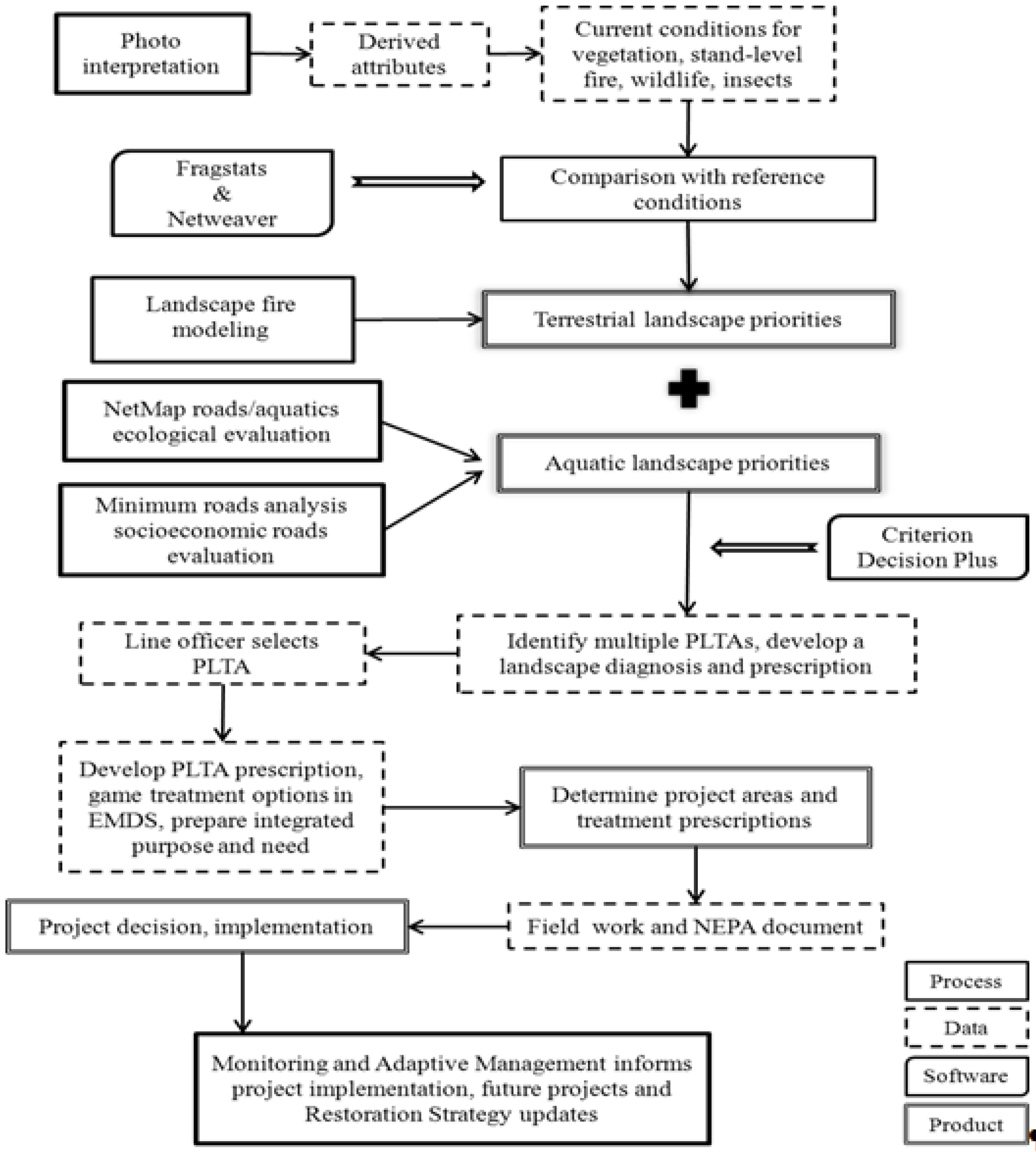
2.1. Overview of the Strategy

For simplicity, the strategy for landscape evaluation was implemented in approximately eight steps:

Step 1—determine the landscape evaluation area,
Step 2—evaluate landscape patterns and departures,
Step 3—determine landscape and patch scale fire danger,
Step 4—identify key wildlife habitat trends and restoration opportunities,
Step 5—identify aquatic/road interactions,
Step 6—evaluate the existing road network,
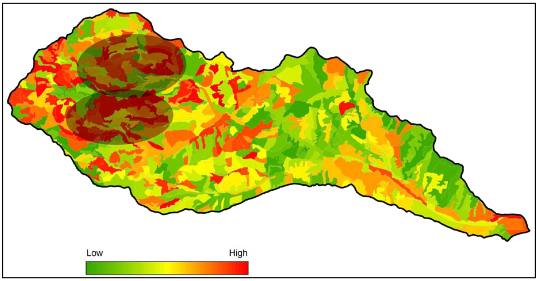
Step 7—identify proposed landscape treatment areas (PLTAs), and
Step 8—refine PLTAs and integrate findings from steps 2–6 into landscape restoration prescriptions.

District specialists from multiple disciplinary fields (see Acknowledgments) worked in partnership to complete each of the steps. Steps 1–6 occurred concurrently and were completed prior to Steps 7 and 8. These steps were applied in the Nile Creek analysis area; we present the landscape-evaluation model for that area.

2.2. Foundations of the Current Study

The present study builds on a body of work by the three senior authors and numerous colleagues over the past 20 years. To avoid burdening this section with great detail on methodologies, descriptions of foundational work on evaluating landscape vegetation patterns and departures can be found in Supplementary Information. Topics covered in the latter include:

(1): A theoretical basis for hierarchical patch dynamics in landscapes (Section 1);
(2): Tool development work for evaluating departures in landscape-level spatial patterns of vegetation with respect to reference variation (NRV, also known as RV), based on hierarchical patch dynamics theory (Section 2); and
(3): An approach to analyzing potential vegetation impacts associated with climate change, based on the concept of reference conditions for analogue climate conditions (Section 3).

In the remainder of this section, we refer the reader to Supplementary Information for detailed accounts of the concepts and methods.

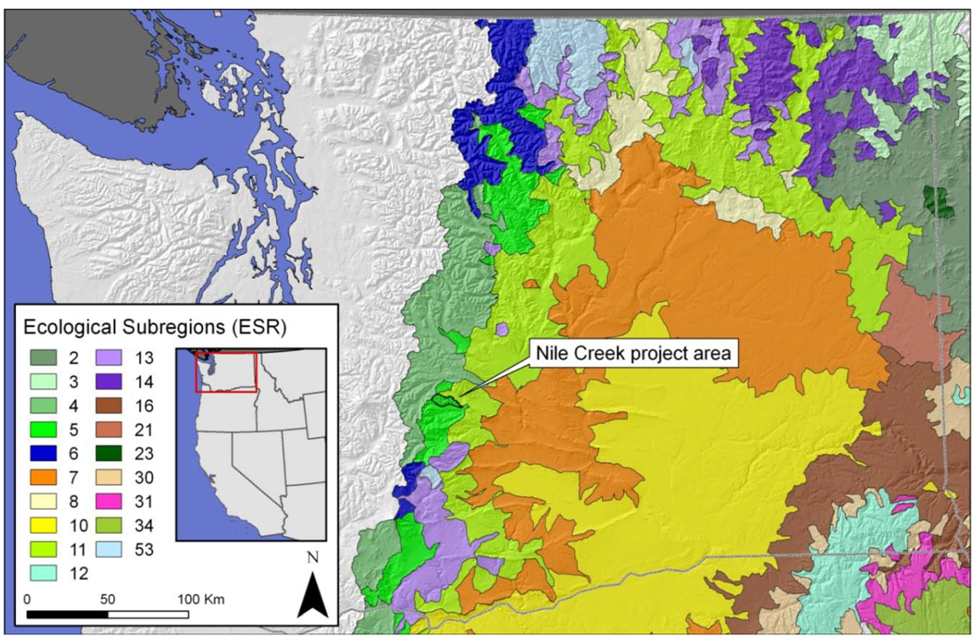
2.3. Determining the Landscape Evaluation Area

Determining the size of the evaluated area had implications for ecological and planning efficiency. Evaluating one or more subwatersheds (12 digit, 6th-field hydrologic unit code, 4000 to 12,000 ha each) was recommended by Reynolds and Hessburg [42], Hessburg et al. [14], and Lehmkuhl and Raphael [43], who showed that some spatial pattern attributes are influenced by the size of the analysis area, especially when areas are too small. We used subwatersheds larger than 4000 ha to avoid this bias. Watershed size also provided a representative range of ecological gradients, elevations, and forest types, and was useful to evaluating the influence of anticipated forest restoration treatments on aquatic habitats and species.

Watershed size was large enough to evaluate many cumulative effects, but wide-ranging wildlife, and most salmonids species required much larger analysis areas than subwatersheds [44,45,46]. Numerous future project areas could be planned via a multi-subwatershed analysis, thereby increasing efficiency, decreasing costs, and increasing rigor of environmental analysis leading to more effective project implementation. The actual project area included three subwatersheds covering an area of ~29,000 ha (Figure 1). For brevity, this paper discusses landscape analysis in just one of these subwatersheds, Nile Creek, which encompasses an area of 8295 ha.

Figure 1. Ecological subregions in eastern Washington, USA, as delineated by Hessburg et al. [47].

2.4. Project Area

The Nile Creek project area is located in ecological subregion (ESR) 5 (Figure 1) of Hessburg et al. [47]. ESR 5 is a relatively warm ecoregion (average annual temperatures range from 5–9 °C), with a moderate solar regime (annual average daylight incident shortwave solar radiative flux ranges from 250–300 W∙m⁻²), a moist but not wet precipitation regime (400–1100 mm/year total annual precipitation), and is predominantly occupied by moist and cold forest types, with dry forests, woodlands, and shrublands in the lowest elevations [47]. The Nile Creek subwatershed lies in the rain shadow east of the crest of the Cascade Mountain Range, where the mean elevation is 1247 m, and elevation ranges from 611 to 1957 m above mean sea level. Most of the precipitation in Nile Creek is derived from snow falling during winter months.

From Figure 2A, it is apparent that the dominant physiognomic condition in the Nile Creek subwatershed is forest, with grass and shrubland patches primarily residing in the lowest elevations, in occasional subalpine meadows, and in subalpine shrub fields remaining after severe historical wildfires not yet recolonized by forest. Shrubland patches are dominated by big sagebrush (Artemisia tridentata) and antelope bitterbrush (Purshia tridentata). Lowland and ridge top dry forests and woodlands are comprised of ponderosa pine (Pinus ponderosa) and Douglas-fir (Pseudotsuga menziesii) in pure or mixed stands (Figure 2B).

Mixed conifer forests reside in the middle elevations, and include ponderosa pine, Douglas-fir, western larch (Larix occidentalis), and western white pine (Pinus monticola) as early seral dominants, and grand fir (Abies grandis), subalpine fir (Abies lasiocarpa), Pacific silver fir (Abies amabilis), and Engelmann spruce (Picea engelmannii) as late successional species (Figure 2B). The uppermost elevations in the watershed support lodgepole pine (Pinus contorta), mountain hemlock (Tsuga mertensiana), subalpine larch (Larix lyalli), and whitebark pine (Pinus albicaulis) forest; however, most of the whitebark pine has been killed by the white pine blister rust fungus (Cronartium ribicola), and only a skeletal remnant remains. Incidental inclusions of western hemlock (Tsuga heterophylla) and western redcedar (Thuja plicata) are found at middle and upper elevations in the watershed, especially in moist to wet, concave landform settings, on small benches, and in valley bottoms.

Figure 2. The Nile Creek Project subwatershed area with maps of existing vegetation conditions by (A) physiognomic type, (B) cover type, (C) structural class, (D) canopy cover (decile) class, (E) late-successional and old forest class (there was no remaining old forest in the subwatershed), (F) western spruce budworm (WSB) vulnerability class, (G) surface fuel loading class, and (H) expected flame length class (90th percentile wildfire burn conditions). Cover types classes are: PIPO = ponderosa pine, LAOC = western larch, PICO = lodgepole pine, PSME = Douglas-fir, ABGR = grand fir, ABAM = Pacific silver fir, ALBA2/PIEN = subalpine fir/Engelmann spruce, TSME = mountain hemlock, PIAL/LALY = whitebark pine/subalpine larch, HDWD = hardwood species, Herbland = grassland species, Shrubland = shrub species, NF/NR = nonforest/non-rangeland cover conditions (rock, water, ice, bare ground). Structural classes are those described and defined in references [14,19,20,22]. Western spruce budworm vulnerability classes were consistent with those defined in [20]. Surface fuel loading classes are: Low (0.0–44.9 Mg/ha), Moderate (45.0–67.3 Mg/ha), High (>67.3 Mg/ha). Flame length classes: Low (0.0–1.2 m), Moderate (1.3–2.4 m), and High (>2.4 m).

The Nile Creek subwatershed was selectively logged several times during the 20th century because historically frequent, low severity fires in the low and middle elevations naturally favored recruitment of abundant large (>63.5 cm dbh) western larch, ponderosa pine, and Douglas-fir. As a result of harvesting, old forest patches have been completely eliminated (Figure 2E), and patches that still retain remnant large trees in the overstory still remain as late-successional structure. As can be seen in Figure 2C, much of the forest structure of the Nile Creek subwatershed is dominated by intermediate-aged (~70–150 yr old) forest conditions displaying open or closed canopy stem exclusion structure, or young multi-story, and understory re-initiation structural conditions. Most stand initiation structures were derived from regeneration harvesting. Canopy cover conditions vary widely as a result of soil moisture and harvest history (Figure 2D), but most of the forest is densely stocked and multi-layered with relatively high canopy cover in comparison with historical conditions. This is the primary signature of eliminating many low and mixed severity fires during the 20th and early 21st centuries.

One of the consequences of repeated selection cutting, fire suppression, and fire exclusion via roads and livestock grazing in Nile Creek has been the effect of those influences on forest succession and disturbance dynamics. Repeated selective logging created canopy gaps with the removal of individual trees and tree groups, enabling a nearly continuous regeneration and release of shade tolerant Douglas-fir, grand fir, and subalpine fir, which are host to the western spruce budworm (Choristoneura occidentalis). The resulting forest structure is dense, multi-layered and highly palatable to this defoliator. Hence, as shown in Figure 2F, the current structure and composition of the Nile Creek forest is vulnerable to ongoing defoliation, top-killing, and mortality losses by budworm. These conditions are also predisposing to tree-killing Scolytid (Coleoptera/Curculionidae/Scolytinae) bark beetles, which are well-adapted to attacking trees stressed and weakened by some other biotic or abiotic agent [12,20,22].

Similarly, selective harvesting created significant slash and surface fuel accumulation after logging (Figure 2G). Likewise, the dense and multi-layered conditions favorable to the budworm also serve as canopy fuels in the event of wildfires. Dense canopies trap heat generated by surface fires, and layered canopies readily convey surface fires to the overstory canopy resulting in both active and passive crown fires. Figure 2H shows the flame lengths (m) that are currently expected under 90th percentile wildfire burn conditions (an average dry summer in the Nile). Under more extreme weather and fuel moisture conditions, some areas of the Nile Creek drainage would burn more severely.

As this narrative suggests, forest conditions in the Nile Creek drainage neither appear nor function as they did even 100 years ago. As a consequence of the current circumstances and a new emphasis by the US Forest Service on restoring vital ecosystem processes and resilience to forest landscapes on public lands [41], The Okanogan-Wenatchee National Forest has refocused its vegetation management efforts on forest restoration [41]. In support of that emphasis, we developed a decision support tool that enables managers to evaluate a myriad of changes to vegetation patterns and associated processes, and use that information to develop landscape prescriptions that would begin the process of landscape restoration.

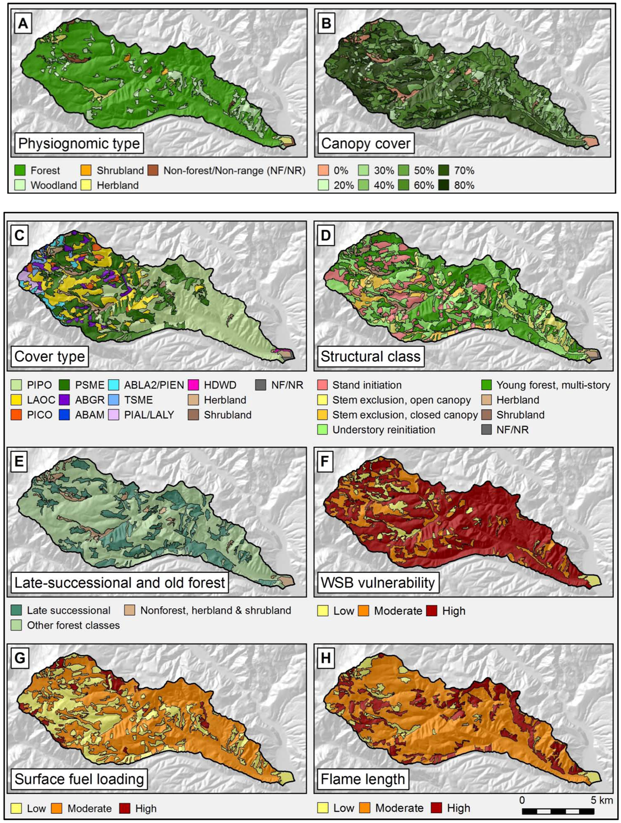
2.5. Evaluating Landscape Vegetation Patterns and Departures

We evaluated vegetation departure of the existing conditions of the Nile Creek subwatershed (a ~8300-ha 12-digit hydrologic unit in the U.S. Geological Survey system [48]) relative to two broad reference ranges of pattern conditions (see Supplementary Information, Section 2, Section 3). One reference range is associated with the early 20th century climate, which we call the NRV or “natural range of variation” conditions. The second reference range is associated with a future warming 21st century climate, which we call the FRV or “future range of variation” conditions. Methods for conducting the departure analysis comparing current conditions to NRV are outlined in Supplementary Information, Section 2. Methods for conducting the departure analysis comparing current conditions to FRV are outlined in Supplementary Information, Section 3, and are analogous to the NRV departure analyses.

The Nile Creek project area (Figure 1) fell in ecological subregion (ESR) 5 of Hessburg et al. [47], and we used the NRV estimates of this ecoregion to represent natural variation in spatial patterns for the pre-management era (~1900, Supplementary Information, Section 1, Section 2). To consider the natural landscape patterns that might occur under a climate-change scenario, we adopted a scenario involving a climatic shift to drier and warmer conditions (FRV), using reasoning described in Gärtner et al. [49], and Supplementary Information, Section 3. Empirical data from the next drier and warmer ecoregion (ESR 11, Figure 1) were used as a reference set to represent the pattern variation of the FRV associated with the analogous climate-change scenario for the project area [47].

Evaluating Landscape Vulnerability to the Western Spruce Budworm

We evaluated the current vulnerability of Nile Creek vegetation to a native defoliating insect, relative to the NRV and FRV ranges, using methods of Hessburg et al. [22,50]. Each patch was assigned a vulnerability class, based on vegetation factors that increased patch vulnerability to the insect. In Nile Creek, we evaluated landscape vulnerability to the western spruce budworm. Western spruce budworm outbreak extent, duration, and severity depend on (1) the amount, structure, quality, and spatial distribution of available host patches, (2) conducive environmental conditions for budworm life stages, and (3) dispersal opportunities to suitable host patches. Large areas that are successionally advanced and have multiple canopy layers of Douglas-fir, grand fir, white fir, and subalpine fir are vulnerable to defoliation by budworm. Warm, dry sites are more vulnerable to budworm outbreaks than are cool mesic sites. Damage associated with this insect had increased over the last several decades and District foresters were interested in understanding the extent and relative severity of the vulnerability increase. The products of this step were maps of patch vulnerability to the western spruce budworm for the current landscapes, which were compared against the two climate reference conditions for these same landscape vulnerabilities.

2.6. Determining Patch and Landscape Scale Fire Danger

Stand or patch-level expected wildfire behavior (90th percentile wildfire burn scenario) was modeled for all current and reference condition patches using methods detailed in Hessburg et al. [22] and Huff et al. [51]. Current wildfire behavior conditions of patches for flame length, rate of spread, fireline intensity, and crownfire potential were evaluated against reference conditions to determine departure from both the NRV and FRV ranges.

We modeled expected landscape-level (compare with patch level) fire behavior consistent with a dry, hot summer wildfire (97th-percentile burn conditions) at the scale of the entire subbasin (8-digit hydrologic unit). In the case of the Nile Creek project area, the Naches subbasin (~180,000 ha), which fully encompasses Nile Creek. Available forest-wide fuels layers were resampled to 90m-resolution rasters and 97th-percentile fuel moisture and weather conditions were used to condition fuels for fire behavior modeling within the FlamMap fire modeling framework ([52] and references therein).

FlamMap is a fire spread model that is used to characterize fire behavior under a constant set of environmental conditions for an entire landscape. Fire behavior calculations are derived from fuel moisture, wind speed, and wind direction data provided in initial model parameterization. FlamMap is designed to examine spatial variability in fire behavior, so fire behavior calculations are performed independently for each cell of a gridded landscape. Spatial inputs to FlamMap include eight GIS raster themes that describe surface and canopy fuels and topography, which are combined into a Landscape (LCP) File. Any raster resolution can be used, but all 8 layers must be co-registered and be identical in resolution and map extent. The user is required to input initial fuel moisture conditions for each standard surface fuel model used, and the fuel model parameters for any customized surface fuel models that are created. Fire behavior is generated for all cells in a landscape using assumed uphill winds, a single constant wind speed and direction combined with slope to produce a fire spread vector, by winds routed in the maximum direction of spread, or by supplying customized wind grids (our chosen method).

There are also options for calculating fuel moistures in FlamMap. One can use a fixed set of fuel moistures for each surface fuel model used (our approach), or fuel moistures can be conditioned by a wind and weather stream that is used to calculate localized moisture contents of 1 and 10-h dead surface fuel size-classes as they are influenced by elevation, slope, aspect, and canopy cover. Basic fire behavior outputs are generated in raster format for surface and crown fire calculations, which can be saved in several image formats. Additionally, the user can request a combined output that displays spread vectors showing the spread rate and maximum spread direction of fires.

Because wind can be highly influential to fireline intensity and the direction of fire spread, we created customized wind grids using WindNinja modeling software [53]. WindNinja is a relatively simple model designed for simulating micro-scale, terrain-influenced winds. WindNinja simulates changes in diurnal wind flow using sensible surface heat flux, distance to ridge top or valley bottom, slope steepness, and surface and entrainment drag parameters to compute diurnal winds. Diurnal wind flow can be combined with the ambient gradient winds.

In consultation with District fire managers, we derived gridded winds in WindNinja for the five most likely prevailing wind directions and used these grids as input to the FlamMap model. We assumed that the likelihood of each prevailing wind direction was approximately equal because the available weather station data were of poor quality and produced results that were contrary to the experience of seasoned local fire managers. For each of the wind directions, the subbasin landscape was ignited with 1000 randomly distributed fire starts 100 times each, and fires were allowed to burn for six hours each until all of the landscape was exposed to ~100,000 total ignitions. Each model run created several raster outputs that were stored for further analysis, including: fireline intensity, active and passive crown fire activity, rate of spread, flame length, and node influence [52].

Node influence is a value assigned to all pixels in FlamMap that represents the number of pixels that burn during the simulations as a result of that pixel burning. Node influence is highly variable, depending on ignition location, fuel arrangement, simulation edge effect, and simulation period. To create a meaningful node influence grid, all of the node influence outputs were composited from all ignitions, and from each wind direction with equal weighting. The layers for flame length and rate of spread were also composited across the five different wind directions.

Finally, the composited node influence layer was combined with the composited flame length and rate of spread layers to create an additive index showing the relative contribution of each pixel to the spread and intensification of fire. Areas with large clusters of high fire danger pixels (i.e., ≥80th percentile scores for combined flame length, node influence, and rate of spread) were identified as priority treatment areas, to strategically interrupt the flow of wildfire across large landscapes. Areas of high fire danger adjacent to the wildland urban interface (WUI) were an especially high priority because of the opportunity to protect human life and property.

2.7. Identifying Wildlife Habitats and Restoration Opportunities for Focal Species

In this evaluation, we: (1) determined the location and amount of habitat for focal wildlife species present within the landscape-evaluation area, (2) compared the current amount and configuration of habitats for focal species to the NRV and FRV reference conditions for these same habitat features, and (3) identified habitat restoration opportunities and priorities that could be integrated with other resource priorities and carried forward into project planning.

The process for selecting focal species is detailed in Suring et al. [54]. In summary, focal wildlife species were selected: (1) from groups of species and represent the habitat associations and risk factors of the group, (2) because of their potential responses to restoration activities, and (3) for this evaluation, as a subset of provincial level species viability assessments [55]. Focal species included the northern spotted owl, the northern goshawk (Accipiter gentilis), the white-headed woodpecker (Picoides albolarvatus), and the American marten (Martes americana). The habitat definitions that were used in the landscape evaluation for these species are detailed in Gaines et al. [56]. The products of this evaluation step were maps showing the location and amount of habitat for each of the focal species, and maps and tabular data showing the degree of departure in habitat amounts and configuration between current and both reference conditions.

2.8. Evaluating Aquatic Ecosystem and Road Interactions

In this step, we identified the road segments that had the greatest impacts on streams, channel features and migration, and in-stream habitats, to determine road restoration priorities. The components of the aquatic/road interactions evaluation were hydrologic connectivity of roads and streams, fish distribution, slope stability and soil properties, and stream channel confinement. These components were evaluated using NetMap [57] and results were incorporated into project planning and alternative comparison. The hydrologic connectivity evaluation ranked the relative importance of flow routes connecting the road system to streams by combining a georeferenced roads layer with a flow-accumulation file generated from a 10-m digital elevation model (DEM). The evaluation of fish distribution linked current in-stream and other survey data with a current streams layer. This would enable later integration in EMDS of potential treatment areas with current fish distributions for listed and sensitive fish species.

Slope and soil stability was modeled by combining an existing soils layer [58,59] with the DEM, and assigning slope breaks of 0–34.9%, 35–60%, and >60%. Unstable soils and steep slopes were located on maps to identify potential slope failure locations and other soil erosion related hazards. Stream-channel confinement was evaluated using a layer developed by the Forest that identified stream channels with <3% gradient within 30-m feet of a road.

2.9. Landscape Analysis and Planning in the EMDS System

2.9.1. Overview of Project Workflow

Figure 3. Project workflow for restoration planning on the Okanogan-Wenatchee National Forest. In the diagram, NetWeaver and Criterium DecisionPlus indicate where these core components of EMDS fit into the overall project workflow. The diagram also indicates how other modeling tools mentioned in the methods section (FRAGSTATS, NetMap, FLAMMAP, and WindNinja) complementary, but external, to EMDS fit into the overall flow.

2.9.2. Logic Processing to Assess Departure

The EMDS application for the Nile Creek project evaluated five primary logic topics in a NetWeaver model. We compared the current landscape to the pre-management era and future warming climate reference conditions (NRV and FRV “reference conditions”, respectively, in Figure 3, Figure 4) in terms of vegetation pattern departure, a major insect vulnerability, patch and landscape level fire behavior attributes, and habitat availability for focal wildlife species. Conditions for NRV were derived from historical reconstructions of vegetation in ESR 5 (Supplementary Information, Section 2, Figure 4). Conditions for FRV (future range of variability) were similarly derived from historical reconstructions, but based on ESR 11, which represented a warmer and drier subregion, whose conditions were analogous to those anticipated with climate warming (Supplementary Information, Section 3, Figure 4). The Landscape Fire topic was evaluated at a subbasin scale. The aquatic-road interactions and minimum roads analysis required Forest-wide modeling efforts, which were in draft at completion time of this project, so abbreviated versions were incorporated in this study, and run outside of the EMDS model.

Combined cover type-structure class (CTxSC) and combined potential vegetation type-cover type-structural class (PVGxCTxSC) conditions were evaluated as subtopics under the primary topic of vegetation pattern departure (Vegetation). These were core vegetation evaluations. The CTxSC evaluation asked—“How have patterns of structural condition across a spectrum of cover types changed as a consequence of management, and how do these changes compare given the historical and future climate conditions as reference”. The PVGxCTxSC evaluation was more complex. It asked the related question—“How are these changes distributed by potential vegetation type?”

The Stand Fire logic network considered contributions to stand-level fire behavior departures; subtopics considered were fuel loading (Loading) and expected 90th percentile wildfire rate of spread (ROS), flame length, risk of crownfire (RCF) and fireline intensity (Intensity) departures. Subtopics considered within the Wildlife logic network were departures in late-successional and old forest abundance (LSOF), and white-headed woodpecker (WHWP) and northern spotted owl (SPOW) habitats. One topic was considered within the Insects and Diseases network; forest vulnerability to the western spruce budworm (WSB). This module in the EMDS tool is currently under expansion to include additional insect and disease vulnerabilities. The Landscape Fire logic network considered contributions to landscape-level fire behavior departures; subtopics included node influence (Sending), fireline intensity (FireInt), and rate of spread considering topography and fuels (Spread).

Figure 4. Five CDP decision models, representing the contributions of logic network evaluations to treatment priority scores (range 0, darkest green to 1, darkest red) in the Nile Creek subwatershed. Acronyms in the figure are as follows: Stand fire = the weighted results of subtopic departure analyses (weights are shown with each topic and subtopic); NRV = the weighted results of all subtopics that evaluate departure from the natural range of variation; ROS = wildfire rate of spread; RCF = risk of crownfire, Loading = surface fuel loading; intensity = fireline intensity; Flame length = flame length; FRV = the weighted results of all subtopics that evaluate departure from the future range of variation; to avoid confusion, an “f” is placed immediately before a subtopic acronym to indicate that it is associated with the FRV portion of a departure analysis; Wildlife = the weighted results of subtopic departure analyses for key wildlife habitat pattern and abundance; LSOF = late successional and old forest; WHWP=white-headed woodpecker; SPOW = northern spotted owl; WSB haz = western spruce budworm hazard departure; CTxSC = departure of combined cover type and structural class conditions; CTxSCxPVG = departure of combined cover type, structural class, and potential vegetation group conditions; Sending, FireInt, and Spread denote the varying degrees of node influence “fire sending”, fireline intensity, and wildfire rate of spread occurring during the FlamMap landscape wildfire simulations.

Each of the NetWeaver subtopics described in the previous paragraph was evaluated with respect to seven class and nine landscape metrics generated by FRAGSTATS [60] (for details on these metrics, see Supplementary Information, Section 2). The class metrics considered each map and asked how patterns within each class, for example, the combined ponderosa pine cover type (CT)-stand initiation structural class (SC), had changed relative to the reference conditions. The landscape metrics asked for each map, how patterns of the entire landscape of all classes had changed in terms of class interspersion, dispersion, contagion, interspersion, juxtaposition, evenness, richness, and the like. Departure of current conditions from the ranges of the two climate reference conditions for the suite of class and landscape metrics formed the basis of vegetation departure analysis.

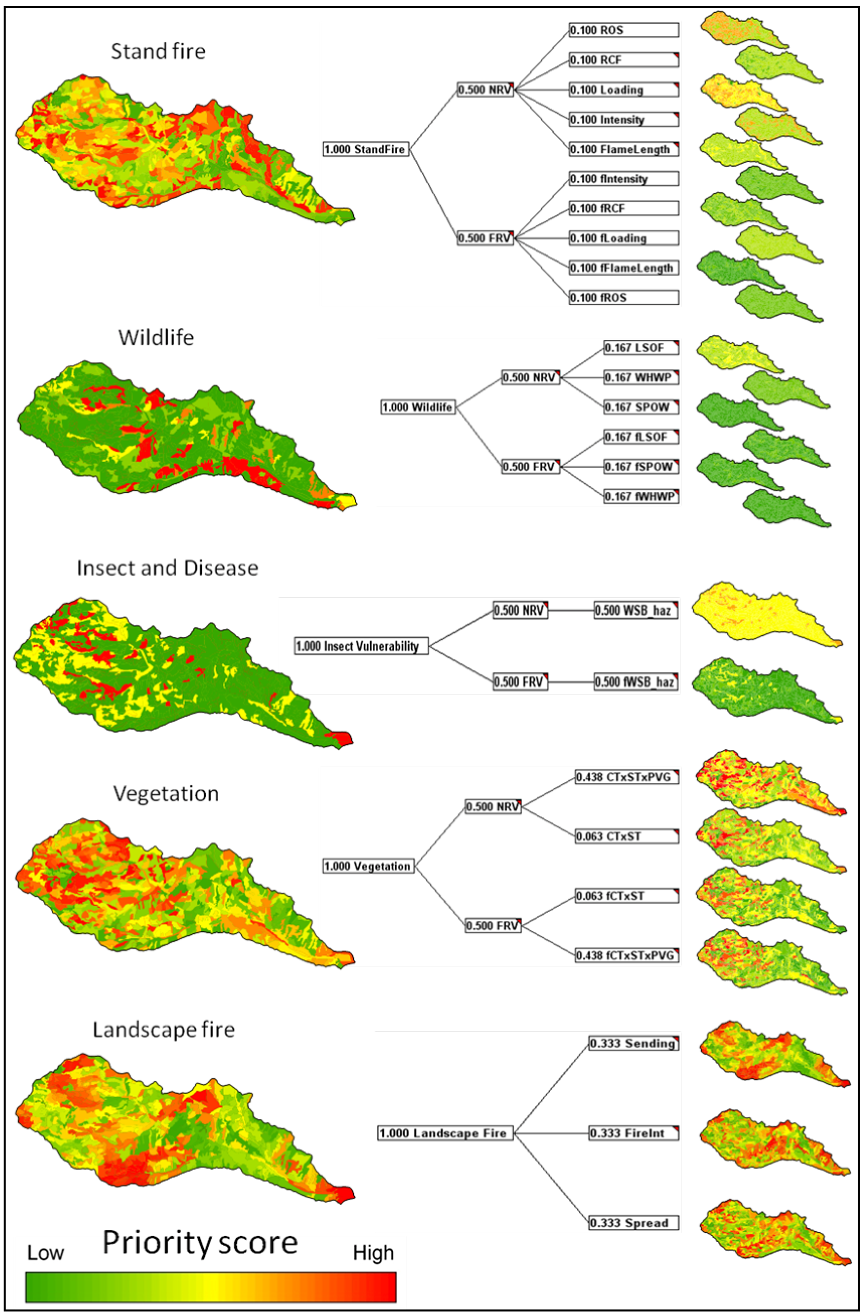
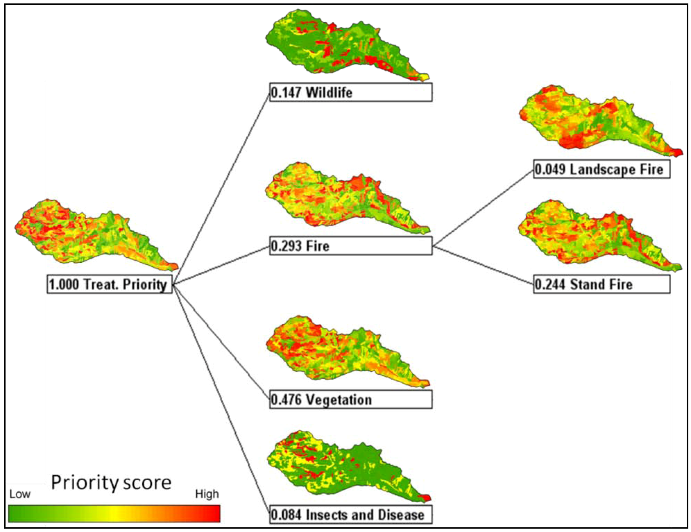
2.9.3. Decision Models to Prioritize Forest Patches for Restoration Treatment

Five decision models, corresponding to the five primary logic topics described in the previous section, were developed in collaboration with the Naches District interdisciplinary team (Figure 4, see also Acknowledgments). With the exception of the decision model for landscape fire, each decision model had departures from NRV and FRV as its primary decision criteria, and these criteria were weighted equally by District disciplinary specialists participating in the project. Subcriteria associated with FRV conditions start with the prefix “f”, and all subcriteria under NRV and FRV evaluations were similarly equally-weighted in the five decision models. Note that all subcriteria in each decision model (Figure 4) are also lowest level criteria, or, in AHP terminology [28,29], attributes, and that each of these decision model inputs corresponds at a NetWeaver output as described previously.

As the final step in the analysis process, a second stage decision model (Figure 5) was designed to derive an overall decision score for treatment priority for the forest patches in a subwatershed, thus integrating the results from the five separate decision models (Figure 4) into one overall priority score for each patch. In contrast to the five separate decision models in which all criteria and subcriteria were equally weighted, in the final composite decision model, managers used the AHP pairwise comparison process [28,29] to specify the relative contribution of each of the component decision models to the overall priority score for a patch.

3. Results

3.1. Departure Analyses

In the Nile Creek subwatershed, the current state of vegetation structure and composition and associated ecosystem processes is more congruent with a future warmer and drier climate than with the historical climate of ESR 5. This result was expected given our knowledge of the local vegetation conditions and management history. The Nile Creek drainage, especially in the low and mid-montane elevations had been heavily managed. Timber harvest and reforestation had favored ponderosa pine to a level that was inconsistent with historical conditions, but that is better adapted to warmer and drier conditions that are expected (Figure 4). Moreover, surface and canopy fuel treatments have been extensive in this same area. The result is a better affinity with the FRV conditions and a poorer one with the NRV conditions. These results are clearly visible when one contrasts the results of NRV and FRV departure analyses for Stand Fire, Vegetation, and Insects and Diseases (Figure 4).

However, this was not observed in the upper montane reaches (western half) of the subwatershed, where departure with the NRV and FRV conditions was most apparent. In these locations, large western larch and Douglas-fir and not ponderosa pine were historically the dominant overstory species. Twentieth century selective harvesting had altered the cover types and structural classes significantly by removing the medium (40.5 to 63.5 cm dbh) and large (>63.5 cm) larch and Douglas-fir from the overstory, and enabling seedling, sapling, pole and small tree-sized Douglas-fir, grand fir, and subalpine fir (<40.5 cm dbh) to regenerate in the understory. Departure analyses found elevated abundance of dense, multi-layered, and intermediate-aged forest structures dominated by shade-tolerant Douglas-fir and grand fir. These conditions represented significant pattern departures from both the NRV and FRV conditions (Figure 4).

Furthermore, 20th-century harvest influences created elevated surface fuel loadings because timber harvest slash was not burned in a number of broad areas. The result can be seen in the Landscape Fire analysis patterns for Sending, Fireline Intensity, and Spread. The greatest opportunity for reducing the likelihood of large wildfires also exists in the western half of the subwatershed.

Figure 4 illustrates the contributions of each of the logic subtopics to the decision scores, for each of the five separate decision models. For the four decision models that consider separate evaluations of NRV and FRV (i.e., for all conditions but Landscape Fire), departure from reference conditions is more pronounced with respect to NRV than FRV. For example, with regard to NRV components, Stand Fire ROS (rate of spread) and Loading (surface fuel loading) exhibited the greatest departure overall, but scattered patches of moderate departure were present in the case of Intensity (fireline intensity) and Flame Length, and these departures are more pronounced than those in the corresponding maps for FRV.

Greater departures from NRV compared to FRV were obvious for LSOF under the Wildlife topic, WSB-haz under the Insect and Disease topic, and CTxSTxPVG under the Vegetation topic. We expect that the difference in LSOF seen in the NRV vs. FRV reference ranges can be accounted for in the likely occurrence of more mixed and high severity fire patches in a warmer drier climate. LSOF patches exhibit the highest surface and canopy fuel loads and moderate to high flame length, fireline intensity, and risk of crownfire conditions under average summer and drier wildfire burn conditions, making them most vulnerable to mortality losses from fire. Likewise, the greater departure of the CTxSTxPVG (combined cover type, structural class, and potential vegetation group conditions) from NRV compared to FRV under the Vegetation topic shows that more large fire tolerant trees and open growing patch level conditions were more apparent historically than is currently the case after 20th century timber harvesting. We have observed similar results in previous work (Supplementary Information, section 3).

3.2. Identifying Priority Treatment Areas

Figure 5 shows the overall score for prioritizing treatments in the Nile Creek drainage considering the weighted contributions of the five separate decision models (Figure 4). Here, we see that departures from both the NRV and FRV climate reference conditions for patch-scale fire (Stand Fire) as well as vegetation departure (Vegetation) and Landscape Fire conditions were major determinants of restoration priority for patches in the subwatershed. For these three decision models, a large proportion of the western half of the Nile Creek subwatershed is rated as moderate to high priority. In contrast, although high priority areas were identified within Nile Creek with respect to the decision models for Wildlife and Insects and Disease, they occurred as relatively scattered patches embedded in a matrix of relatively low priority areas.

Figure 5. Second stage CDP decision model for the Nile Creek subwatershed of the Nile project area. Landscape treatment priority scores of polygons within the Nile Creek subwatershed (range 0, darkest green to 1, darkest red) were derived from primary criteria associated with four major topics (see also Figure 4): Wildlife, Fire, Vegetation, and Insects and Diseases. Primary criteria were weighted by managers using the AHP pair-wise comparison process. Under the Fire criterion, the Landscape Fire and Stand Fire networks (Figure 4) were evaluated as subcriteria, and weighted by District managers. The map on the far left shows the results of the entire CDP evaluation of priority treatment scores assigned to patches. These scores are later used for identifying proposed landscape treatment areas (PLTAs, Figure 6) and potential restoration treatment locations.

Taking a closer look at the overall priority scores for restoration from Figure 5, we see that the density of high priority patches varies substantially over the Nile Creek subwatershed, with highest densities apparent in the western half. Results of the landscape evaluation process thus not only enabled the District planning team to attach a treatment priority and rationale to all patches in each subwatershed, but to identify areas with clusters of high priority patches, termed potential landscape treatment areas (PLTAs), that could form the nucleus of project areas. In Figure 6, we highlight nuclei for two mapped PLTAs in the Nile Creek subwatershed. The encircled areas represent approximate PLTAs emerging from the landscape evaluation. District specialists further refined these PLTAs as they delved into the supporting analysis and information coming from the roads and hydrology analyses conducted outside of the EMDS model. (Note: We are in the process of incorporating road and aquatic analyses into a revised tool.)

The results of evaluations of each primary logic topic provided information that could be used by all members of the interdisciplinary planning (IDT) team to develop a prescription for each landscape (i.e., a landscape-level prescription). For example, results generated from the landscape pattern, fire, and wildlife habitat evaluations allowed the IDT to quantify the amount, types, and spatial locations of treatments to accomplish multiple restoration objectives. These objectives included strategically altering large scale fire behavior, enhancing the sustainability of key wildlife habitat networks, restoring ecosystem functions by restoring landscape pattern and process interactions, reducing risk to human communities, and the minimum road network needed to access treatment areas while reducing the negative impacts of roads on aquatic habitats.

Figure 6. Nile Creek subwatershed patch-level priority scores resulting from CDP evaluation of subcriteria (Figure 4, Figure 5) in EMDS. Landscape treatment priority scores of polygons within the Nile Creek subwatershed (range 0, darkest green to 1, darkest red) were derived from primary criteria associated with four major topics (see also Figure 5): Wildlife, Fire, Vegetation, and Insects and Diseases. Circles show example potential landscape treatment areas (PLTAs) where restoration projects (shaded areas) might focus treatments appropriate to the need, to achieve multi-way and multi-level restoration goals.

Upon completion of the initial landscape evaluation, identification of the PLTAs, and preferred landscape treatment options proposed, vegetation, fuels, and associated data were edited to reflect the effects of virtually applied treatments. These edited landscapes could then be evaluated within the EMDS application and managers could determine the degree to which progress could be made toward restoration goals. That is, each alternative management scenario could be evaluated in EMDS, compared against the NRV and FRV conditions, evaluated for its wildfire and insect vulnerability, and the extent to which wildlife habitats had been improved. In this way, alternatives could be gamed in the model and evaluated side by side for their merits and demerits prior to any implementation. Using EMDS, the IDT was able to evaluate a variety of landscape prescriptions and treatment options, and assess how the various options would affect fish habitats, insect and disease risks, landscape patterns, and the flammability of the larger landscape. The final product was a refined map of PLTAs and a preferred alternative for landscape treatment for the Nile Creek project area. Key attributes of the preferred alternative are discussed below. The process of landscape evaluation provided important advantages to environmental analysis in terms of transparency, efficiency, and credibility. We expand on these points below, as well.

3.3. Benefits of Using the EMDS Decision Support Application

3.3.1. Multi-Resource Planning on an Equal Footing

One of the primary benefits of developing spatially accurate GIS map layers for a common area with varying ecological and manmade conditions, habitats, processes, and infrastructure is that a large cross-section of conditions can be simultaneously considered on an equal footing. In the past, the person with the best hand drawn maps and (often) the loudest voice generally made the greatest mark on an IDT project. But GIS mapping and decision support tools present the ability to change that dynamic. Now, roads and trails, culverts, and road crossings can be considered in the context of changes in the vegetation patterns, and vulnerability to insects, pathogens, and wildfires. In the Nile Creek project, for example, human settlements and infrastructure were located in the extreme low elevations to the east. Examination of the Stand Fire and Landscape Fire conditions enabled District fuel managers and all IDT members to clearly understand the locations of any needed fuel treatments relative to protecting nearby WUI. They all could understand and visualize how these treatments would influence each resource and habitat condition under consideration by the model.

3.3.2. Integration of Resource Values and Conditions

In the recent past, stakeholders and other resource professionals took issue with each other’s assessments of existing conditions. It was difficult to get good data and incorporate it into maps in a combined geodatabase, where layers could be overlain with one another and compared at will. Much of what was discussed in project level planning was based on field reconnaissance notes, professional judgment, hand-drawn maps, or grease pencil drawings on Mylar aerial photo overlays. In the present study, resource professionals developed ortho-rectified GIS maps of each resource or ecological condition they were bringing to the table. For example, the fuels management specialist had surface fuelbeds, canopy bulk density, crown base height, stand height, and tree height maps to use and could discuss how these would drive fire behavior in each patch and on the landscape. The wildlife biologist translated these same conditions into habitat classifications for white-headed woodpecker and spotted owl using nesting, roosting, and foraging characteristics needed in forest patches and nearby neighborhoods. The silviculturist translated these same conditions into patterns of forest structure and composition, both existing and desired. In this way, the EMDS tool could truly integrate the conditions as though they were facets of the same stone. One could see that when one characteristic was changed in a habitat condition for a bird, the fuel bed, forest structure, and fire behavior might also change. This enabled the IDT to notice and discuss trade-offs they were willing to make as they considered alternative management scenarios.

3.3.3. Transparency of Evaluations

Another useful quality of the EMDS application is its ability to transparently display how each evaluation result is derived. For example, in a PLTA, if a collection of patches was rated as high priority for treatment, as in Figure 6, each IDT member could look on-screen at the computer display of the priority scores, click on any patch, and move down each level of the logic network to determine which conditions were most departed, or in the poorest state. This utility gave IDT members unambiguous insight into what drove the priority score of each patch, and what must be restored to elevate the score and remedy conditions. This enabled IDT members and stakeholders to understand what was evaluated, what the outcomes were, and where the remedies would most likely occur.

3.3.4. Conserving More Rather Than Fewer Options

One of our goals in developing a decision support tool for landscape evaluation was to develop project level management plans that could restore more resilient landscapes that had more rather than fewer options for the future. The IDT could see that settlement and management changed historical conditions to the present. Restoring the habitat patterns and functionality of the past would improve resilience a great deal, but it would not result in the most resilient landscape conditions; the climate is warming and drying in eastern Washington. To conserve the greatest number of options for landscapes we incorporated the NRV and FRV departure evaluations into the model. Landscape restoration prescriptions with the best opportunity to improve resilience would be those whose range of patterns fell with the NRV and the FRV ranges. This was readily possible because for most landscape measures, there was a high degree of overlap in these ranges.

4. Discussion and Conclusions

4.1. The Selected Project Alternative

In the beginning of this paper, we discussed a succession of settlement and management influences that had dramatically altered the structure and functioning of eastern Washington landscapes. The Nile Creek subwatershed was no exception. It had been repeatedly logged and ecologically speaking, it was dysfunctional in a number of ways. Still, in other ways, much good work had been done. Landscape analysis showed the IDT that they were dealing with a mixed bag.

The final alternative selected and implemented by the IDT accomplished a number of key results supported by the landscape analysis. Chief among them were:

(1)

Development of several projects in the western half of the subwatershed that reduced vulnerability to wildfires and budworm defoliation, improved vegetation resilience to climatic warming, and decreased fragmentation by increasing patch sizes.

a.: These projects emphasized restoring stronger topographic controls on species composition, tree density, and fuelbeds, by tailoring treated patches to north and south aspects and their inherent size distribution.
b.: Southerly aspects were thinned to lower stocking levels where the largest western larch and occasional Douglas-fir were favored, and where worst Douglas-fir dwarf mistletoe (Arceuthobium douglasii) infested trees were removed. Surface fuels and fuel ladders were also reduced by prescribed burning.
c.: Understory thinning was accomplished using variable retention methods like those described by Larsen and Churchill [61], and Churchill etal. [62]. The resulting patch conditions exhibited a fine scale heterogeneity that included uneven spacing of individual trees and variable sized tree clumps, with variably sized gaps in between them. This was an example of fine scale heterogeneity within patches being incorporated among meso-scale patches.
d.: Northerly aspects were allowed to carry higher stocking density and more layered canopy conditions in favor of maintaining spotted owl habitat.
e.: Surface fuels treatments were prescribed outside of but adjacent to a number of the best identified spotted owl habitats to increase the likelihood of their persistence in the event of wildfire.
f.: White-headed woodpecker habitats were favored on southerly slopes at the forest and woodland ecotone, and on drier ponderosa pine sites, by maintaining large ponderosa pine trees and snags, and by recruiting more of the same for the future. Future stands will become park-like ponderosa pine, old forest single story patches.
g.: The project was accomplished without harvesting large and old trees, in order to increase the amount of future old forest and late-successional habitat, and the abundance of future large snags and down logs, which the project identified were already in short supply.

(2)

Development of several prescribed burning projects in the eastern half of the subwatershed that reduced vulnerability to wildfires and reduced crown fire hazard in favor of protecting downstream WUI conditions with high certainty.

h.: Burn prescriptions were applied over several hundred hectares, especially on southerly aspects, breaking up continuous surface fuel beds, and favoring retention of the largest fire tolerant ponderosa pine.
i.: Topography was used to intuitively tailor treated areas.

Overall, the project moved the Nile Creek landscape toward conditions that resembled the inherent variability associated with the pre-management era conditions and those that are expected with climatic warming in this area.

4.2. What Worked Well?

First and foremost, development of the EMDS application improved communication within the IDT, because it gave the members a concrete framework and equal footing for organizing the analytical and decision space necessary for exploring restoration management opportunities. Resource managers were able to organize the logic and analysis needs for their area of expertise and share their sub-models with the IDT as primary topics that can feed into the overall application structure.

The use of EMDS in this application allowed for better integration across resource disciplines and yielded repeatable landscape evaluation and decision-making processes. The alternative development portion of the process allowed the IDT to identify priority areas for restoration treatments that could achieve multiple objectives. The comparison of current conditions to NRV and FRV conditions in EMDS enabled the IDT to develop objective measures that could be used to describe resilient landscapes and measure progress towards achieving the restoration goals. Integration of a climate change scenario into EMDS based on the approach described in Gärtner et al. [49] enabled a concrete application of current climate-change science into the landscape evaluation process, which informed project-level planning and decision-making, and implemented an important climate adaptation [63].

The landscape evaluation allowed the IDT and the decision-maker to strategically locate project areas to meet multiple restoration objectives, while keeping what was in good condition and creating an expanding area of similarly good conditions. In addition, EMDS provided a mechanism to display how emphasizing a certain resource more than another would influence treatment prioritization, the spatial allocation of treatments, and the distributed effects on other resources and conditions.

To date, no other planning process has allowed managers on the Okanogan-Wenatchee National Forest to strategically and spatially locate treatments based on the complex and simultaneous interactions of multiple landscape conditions and resource variables. Managers were better able to describe restoration needs at a landscape scale rather than simply forest stand by forest stand. As a result, new opportunities for restoration treatments were discovered. For example, the District IDT chose a PLTA in mesic forests to address patch types and arrangements rather than solely focused on thinning in dry forests, which had occupied much of the focus in the preceding decade.

The IDT was also better able to integrate concerns for multiple resources. Previously, projects were largely driven by the need to manipulate vegetation for “forest health improvement” and “wildfire mitigation”. The landscape evaluation process more fully integrated planning, simultaneously emphasizing wildlife and aquatic habitat conditions, landscape and patch scale fire behavior, vegetation and fuels patterns, and road-aquatic interactions, leading to restoration opportunities for a multiplicity of resources. The Nile Creek Project became a good example of simultaneous problem-solving rather than an exercise in trade-off analysis.

4.3. What Could Be Improved?

Relatively simple CDP decision models were developed in this EMDS application for want of time and additional resources. Alongside of information reflecting knowledge about the state of the system, decision criteria reflecting social values and other feasibility and efficacy criteria important to decision-making might have been included. Examples of such criteria might include consideration of fire risks to human infrastructure in the wildland-urban interface, effects on meeting other resource objectives where restoration is not the primary goal, matters of technical and economic feasibility and social acceptability, relationships to life-cycle costs and benefits, retreatment frequency, and the duration of positive treatment effects, uncertainties associated with management outcomes and data quality, and trade-offs associated with more or less strategic placement of treatments. We anticipate building in these utilities as additional projects are undertaken, and as relevant data become available.

4.4. Research Opportunities

Two opportunities for increasing the research and heuristic value of this project- level planning tool would include (1) adding stochastic succession and disturbance simulations of landscape treatment prescriptions, and (2) evaluating alternative landscape prescriptions against FRV conditions representing several plausible future climate scenarios. In the first instance, stochastic behavior could be added to modeled landscape-treatment scenarios by simulating them spatially in models, such as the Landscape Succession and Disturbance Model—LANDSUM [64,65], the LADS [66], or LANDIS [67] models. For example, LANDSUM provides state-transition models for the potential vegetation types of a study area. Within each state-transition model are successional states defined by cover types and structural classes, a complete set of transition pathways that show all potential succession paths between states, and transition times related to each potential path. Initialized disturbance probabilities by disturbance severity determine the likelihood that any state will transition to any other state. In this context, landscape treatments would occur as prescribed, but other unplanned disturbances caused by wildfires, forest insects, and forest pathogens could occur as well. The net result would be annualized depictions of planned and unplanned vegetation outcomes, which would be a more accurate depiction of likely outcomes of implemented scenarios.

In a related manner, a range of climatic futures could also be simulated using a “climatized” version of LANDSUM [68] or a similar succession and disturbance model. Simulations would occur as described above, but in this case the conditioning climate would influence fire probabilities by means of a scalar applied to historical fire probabilities assigned from the literature. The advantage of this sort of approach would be in developing hedging strategies for landscape management in an uncertain climatic future.

Another possibility for future research would side-by-side comparison of the usefulness of continuous gradient-oriented wildlife habitat models with patch mosaic models. While it appears that some species and processes respond to ecological and environmental gradients of conditions [69,70], others apparently respond to patch mosaics [71,72]. As such models become available for regional and local species, we would hope to base evaluations of landscape conditions and alternatives on both approaches, and prepare project alternatives that can directly evaluate alternative hypotheses about how factors and their spatial orientation drive species responses. In this context, ongoing monitoring would be essential to hypothesis testing.

4.5. A Low Cost Alternative to EMDS?

EMDS was built as an extension to ArcGIS in large part to take advantage of the powerful geoprocessing capabilities of this GIS environment. As a spatial DSS, EMDS application developers and users routinely make use of ArcGIS geoprocessing features for both pre- and post-processing in the course of application development. However, we recognize that the cost of acquiring ArcGIS can be a barrier to potential developers and users interested in spatial DSS technologies. Although we are not aware of any free or public domain spatial DSS that are comparable to EMDS in terms of functionality, we can suggest GeoNetWeaver (from Rule of Thumb, Inc.) as a low cost alternative.

4.6. Conclusions

Some readers will be curious about the level of effort needed to fully implement decision-support applications for landscape analysis such as that presented in our example. Put simply, the effort can be daunting if the process must begin with collection of field data or new satellite data. As a very rough guide, we suggest that each day of modeling and analysis is supported by 10 days of geoprocessing, and each day of geoprocessing is supported by 10 days of collecting and processing field data. In other words, designing, implementing, and running a landscape DSS typically represents the smallest fraction of the overall effort. On the other hand, if the needed data are already at hand, additional investment in DSS development can return disproportionately large value-added relative to the additional investment required.

There are at least a few strategic lessons to be gleaned from our example. Addressing questions about ecosystem integrity or landscape departure with respect to vegetation required high-dimensional logic representations in order to adequately address the facets of structure and composition. All the logic models discussed collectively evaluated 100s of input variables and 1000s of parameters. Contributing to the very large size of these models, seven class metrics were used to evaluate each patch type, and nine landscape metrics were used to evaluate the spatial properties of the mosaic of patch types. As a practical matter, we consider that the utility of the metrics chosen is entirely dependent upon the questions being addressed. This study demonstrated how decision models can usefully augment the logic-based analysis, thereby introducing practical management issues into the priority setting process, while simplifying the analysis by decomposing it into two relatively simpler problems—understanding the status of the systems in question, and then asking what might be done given the condition of the systems.

Finally, we conclude with a few thoughts on the success of our landscape applications. Our first two examples (Supplementary Information) were primarily developed as proofs of concept in research and development. From an internal perspective, we consider these applications successful in terms of providing an interpretation and synthesis of large volumes of information that we think usefully encapsulated scientific understanding of large, complex, and abstract problems. Of course, the “acid test” for decision-support applications is that managers find them useful, understand them, and actually put them into service addressing real-world management problems more effectively than before. Our main example of project-level planning was successful in these terms.

This landscape evaluation tool is now being implemented on all seven Districts of the Okanogan-Wenatchee National Forest, on an area of more than 1.6 million ha, prior to implementing any landscape restoration project under its Strategy. Moreover, between the draft and final stages of this paper, the US Fish and Wildlife Service in their Revised Recovery Plan and Critical Habitat Rule (CHR) for the northern spotted owl recommended that methods such as ours can serve as an example of how to assess and restore ecological patterns and processes to eastern Washington and Oregon forest landscapes [73,74].

Supplementary Material

Supplementary information can be accessed at:

https://www.mdpi.com/2071-1050/5/3/805/s1.

Acknowledgments

We gratefully acknowledge the Naches Ranger District interdisciplinary team (IDT) for all of their fine work in data development, analysis, and landscape planning, and especially for allowing us to use them as guinea pigs when prototyping these new methods. Special thanks go to Jim Bailey—IDT Leader/Fire & Fuels/Air Quality analysis, Jacquie Beidl—Archaeologist/Heritage Resources analysis, Barry Collins—Engineering/Road Management analysis, Bill Garrigues—Hydrology/Soils analysis, Jodi Leingang—Invasive Species/Understory Vegetation/Range analysis, Dave Lucas and Miles Porter—Timber Sale Layout and Design, Phil Monsanto and Chris Ownby—Silviculture/Landscape Evaluation/GIS Analysis, Matt Dahlgreen—Silviculture, field validation, and landscape prescription development, Sue Ranger—Recreation/Visual Resources analysis, Joan St. Hilaire—Wildlife analysis, Gary Torretta—Fisheries analysis, and Irene Davidson—District Ranger. We are grateful for the reviews of three anonymous referees whose comments substantially improved the manuscript.

Conflict of Interest

The authors declare no conflict of interest.

References

Pyne, S.J. Fire in America: A Cultural History of Wildland and Rural Fire; University of Washington Press: Seattle, WA, USA, 1982; p. 680. [Google Scholar]
Sauer, C.O. Sixteenth Century North America: The Land and the People as Seen by the Europeans; University of California Press: Berkeley, CA, USA, 1971; p. 19. [Google Scholar]
White, R. It’s Your Misfortune and None of My Own: A New History of the American West; University of Oklahoma Press: Norman, OK, USA, 1991; p. 644. [Google Scholar]
White, R. Discovering nature in North America. J. Am. Hist. 1992, 79, 874–891. [Google Scholar] [CrossRef]
White, R. Indian Land Use and Environmental Change. In Indians, Fire, and the Land in the Pacific Northwest; Boyd, R., Ed.; Oregon State University Press: Corvallis, OR, USA, 1999; pp. 36–49. [Google Scholar]
Robbins, W.G. Colony and Empire: The Capitalist Transformation of the American West; University Press of Kansas: Lawrence, KS, USA, 1994; p. 255. [Google Scholar]
Robbins, W.G. Landscapes of Promise: The Oregon Story,1800–1940; University of Washington Press: Seattle, WA, USA, 1997; p. 392. [Google Scholar]
Robbins, W.G. Landscape and Environment: Ecological Change in the Intermontane Northwest. In Indians, Fire, and the Land in the Pacific Northwest; Boyd, R., Ed.; Oregon State University Press: Corvallis, OR, USA, 1999; pp. 219–237. [Google Scholar]
Hessburg, P.F.; Agee, J.K. An environmental narrative of Inland Northwest U.S. forests 1800–2000. For. Ecol. Manag. 2003, 178, 23–59. [Google Scholar] [CrossRef]
Langston, N. Forest Dreams, Forest Nightmares: The Paradox of Old Growth in the Inland Northwest; University of Washington Press: Seattle, WA, USA, 1995; p. 368. [Google Scholar]
Van Wagtendonk, J.W. The history and evolution of wildland fire use. Fire Ecol. 2007, 3, 3–17. [Google Scholar] [CrossRef]
Hessburg, P.F.; Mitchell, R.G.; Filip, G.M. Historical and Current Roles of Insects and Pathogens in Eastern Oregon and Washington Forested Landscapes; Gen. Tech. Rep. PNW-GTR-327; U.S. Department of Agriculture, Forest Service, Pacific Northwest Research Station: Portland, OR, USA, 1994; p. 72.
Hummel, S.; Agee, J.K. Western spruce budworm defoliation effects on forest structure and potential fire behavior. Northwest Sci. 2003, 77, 159–169. [Google Scholar]
Hessburg, P.F.; Agee, J.K.; Franklin, J.F. Dry forests and wildland fires of the inland Northwest USA: Contrasting the landscape ecology of the pre-settlement and modern eras. For. Ecol. Manag. 2005, 211, 117–139. [Google Scholar] [CrossRef]
McKenzie, D.; Gedalof, Z.; Peterson, D.L.; Mote, P. Climatic change, wildfire, and conservation. Cons. Bio. 2004, 18, 890–902. [Google Scholar] [CrossRef]
Westerling, A.L.; Swetnam, T.W. Interannual and decadal drought and wildfire in the western United States. EOS Trans. AGU 2003, 84, 554–555. [Google Scholar]
Westerling, A.L.; Hidalgo, H.G.; Cayan, D.R.; Swetnam, T.W. Warming and earlier spring increase western U.S. forest wildfire activity. Science 2006, 313, 940–943. [Google Scholar]
Moritz, M.A.; Hessburg, P.F.; Povak, N.A. Native Fire Regimes and Landscape Resilience. In The Landscape Ecology of Fire; McKenzie, D., Miller, C., Falk, D.A., Eds.; Springer: New York, NY, USA, 2011; pp. 51–86. [Google Scholar]
Hessburg, P.F.; Smith, B.G.; Salter, R.B. Detecting change in forest spatial patterns. Ecol. Appl. 1999, 9, 1232–1252. [Google Scholar] [CrossRef]
Hessburg, P.F.; Smith, B.G.; Kreiter, S.D.; Miller, C.A.; Salter, R.B.; McNicholl, C.H.; Hann, W.J. Historical and Current Forest and Range Landscapes in the Interior Columbia River Basin and Portions of the Klamath and Great Basins: Part I: Linking Vegetation Patterns and Landscape Vulnerability to Potential Insect and Pathogen Disturbances; Gen. Tech. Rep. PNW-GTR-458; U.S. Department of Agriculture, Forest Service, Pacific Northwest Research Station: Portland, OR, USA, 1999; p. 357.
Hessburg, P.F.; Smith, B.G.; Salter, R.B. Using Natural Variation Estimates to Detect Ecologically Important Change in Forest Spatial Patterns: A Case Study of the Eastern Washington Cascades; PNW Res. Pap. PNW-RP-514; U.S. Department of Agriculture, Forest Service, Pacific Northwest Research Station: Portland, OR, USA, 1999; p. 65.
Hessburg, P.F.; Smith, B.G.; Salter, R.B.; Ottmar, R.D.; Alvarado, E. Recent changes (1930’s–1990’s) in spatial patterns of interior northwest forests, USA. For. Ecol. Manag. 2000, 136, 53–83. [Google Scholar] [CrossRef]
Millar, C.I.; Stephenson, N.L.; Stephens, S.L. Climate change and forests of the future: Managing in the face of uncertainty. Ecol. Appl. 2007, 17, 2145–2151. [Google Scholar] [CrossRef]
Stephens, S.L.; Millar, C.I.; Collins, B.M. Operational approaches to managing forests of the future in Mediterranean regions within a context of changing climates. Environ. Res. Letters 2010, 5, 024003. [Google Scholar] [CrossRef]
Reynolds, K.M.; Rodriguez, S.; Bevans, K. User Guide for the Ecosystem Management Decision Support System, Version 3.0; Environmental Systems Research Institute: Redlands, CA, USA, 2003; p. 89. [Google Scholar]
Miller, B.J.; Saunders, M.C. The NetWeaver Reference Manual; Pennsylvania State University: College Park, PA, USA, 2002; p. 55. [Google Scholar]
Halpern, D.E. Thought and Knowledge: An Introduction to Critical Thinking; LawrenceErlbaum Associates: Hillsdale, NJ, USA, 1989; p. 517. [Google Scholar]
Saaty, T.L. Multicriteria Decision Making: The Analytical Hierarchy Process; RWS Publications: Pittsburgh, PA, USA, 1992; p. 321. [Google Scholar]
Saaty, T.L. Fundamentals of Decision Making and Priority Theory with the Analytical Hierarchy Process; RWS Publications: Pittsburgh, PA, USA, 1994; p. 527. [Google Scholar]
Edwards, W. How to use multi-attribute utility measurement for social decision making. IEEE Trans. Syst. Man Cybern. Syst. Hum. 1977, 7, 326–340. [Google Scholar] [CrossRef]
Edwards, W.; Newman, J.R. Multi-Attribute Evaluation; Sage: Beverly Hills, CA, USA, 1982; p. 336. [Google Scholar]
Stolle, L.; Lingnau, C.; Arce, J.E. Mapeamento da Fragilidade Ambiental em Areas de Plantios Florestais. In Anais XIII Simpósio Brasileiro de Sensoriamento Remoto (in Portuguese), Florianópolis, Brasil, 21–26 April 2007; INPE: Florianópolis, Brazil, 2007; pp. 1871–1873. [Google Scholar]
Girvetz, E.; Shilling, F. Decision support for road system analysis and modification on the Tahoe National Forest. Environ. Manag. 2003, 32, 218–233. [Google Scholar] [CrossRef]
Janssen, R.; Goosen, H.; Verhoeven, M.L.; Verhoeven, J.T.A.; Omtzigt, A.Q.A.; Maltby, E. Decision support for integrated wetland management. Environ. Model. Softw. 2005, 30, 215–229. [Google Scholar]
Wang, J.; Chen, J.; Ju, W.; Li, M. IA-SDSS: A GIS-based land use decision support system with consideration of carbon sequestration. Environ. Model. Softw. 2010, 25, 539–553. [Google Scholar] [CrossRef]
Staus, N.L.; Strittholt, J.R.; Dellasala, D.A. Evaluating areas of high conservation value in Western Oregon with a decision-support model. Cons. Bio. 2010, 24, 711–720. [Google Scholar] [CrossRef]
USDI, Final Draft Recovery Plan for the Northern Spotted Owl; U.S. Department of the Interior: Washington, DC, USA, 1992; Volumes 1 and 2.
USDA, Record of Decision for the Amendments to Forest Service and BLM Planning Documents within the Range of the Northern Spotted Owl and Standards and Guidelines for Management of Habitat for Late-Successional and Old-Growth Forest within the Range of the Northern Spotted Owl; U.S. Department of Agriculture, Forest Service: Portland, OR, USA, 1994.
ROD, Record of Decision for Amendments to Forest Service and Bureau of Land Management Planning Documents within the Range of the Northern Spotted Owl; GPO 1994–589–111/0001; U.S. Government Printing Office, Region No. 10: Washington, DC, USA, 1994.
White, M.D.; Heilman, G.E., Jr.; Stallcup, J.E. Science Assessment for the Sierra Checkerboard Initiative; Conservation Biology Institute: Encinitas, CA, USA, 2005. [Google Scholar]
USDA Forest Service (USDA-FS). The Okanogan-Wenatchee National Forest Restoration Strategy: Adaptive ecosystem management to restore landscape resiliency. 2010. Available online: http://www.fs.fed.us/r6/wenatchee/forest-restoration/ (accessed on 12 January 2011).
Reynolds, K.M.; Hessburg, P.F. Decision support for integrated landscape evaluation and restoration planning. For. Ecol. Manag. 2005, 207, 263–278. [Google Scholar] [CrossRef]
Lehmkuhl, J.F.; Raphael, M.G. Habitat patterns around northern spotted owl locations on the Olympic Peninsula Washington. J. Wildl. Manag. 1993, 57, 302–315. [Google Scholar] [CrossRef]
Ager, A.A.; Finney, M.A.; Kerns, B.K.; Maffei, H. Modeling wildfire risk to northern spotted owl (Strix occidentalis caurina) habitat in central Oregon, USA. For. Ecol. Manag. 2007, 246, 45–56. [Google Scholar] [CrossRef]
Gaines, W.L.; Singleton, P.H.; Ross, R.C. Assessing the Cumulative Effects of Linear Recreation Routes on Wildlife Habitats on the Okanogan and Wenatchee National Forests; Gen. Tech. Rep. PNW-GTR-586; U.S. Department of Agriculture, Forest Service, Pacific Northwest Research Station: Portland, OR, USA, 2003; p. 79.
Reeves, G.H.; Benda, L.E.; Burnett, K.M.; Bisson, P.A.; Sedell, J.R. A disturbance-based ecosystem approach to maintaining and restoring freshwater habitats of evolutionarily significant units of anadromous salmonids in the Pacific Northwest. Am. Fish. Soc. Symp. 1995, 17, 334–349. [Google Scholar]
Hessburg, P.F.; Salter, R.B.; Richmond, M.B.; Smith, B.G. Ecological subregions of the Interior Columbia Basin, USA. Appl. Veg. Sci. 2000, 3, 163–180. [Google Scholar] [CrossRef]
Seaber, P.R.; Kapinos, P.F.; Knapp, G.L. Hydrologic Unit Maps; Water-Supply Paper 2294; U.S. Geological Survey: Washington, DC, USA, 1987.
Gärtner, S.; Reynolds, K.M.; Hessburg, P.F.; Hummel, S.S.; Twery, M. Decision support for evaluating landscape departure and prioritizing forest management activities in a changing environment. For. Ecol. Manag. 2008, 256, 1666–1676. [Google Scholar] [CrossRef]
Hessburg, P.H.; Smith, B.G.; Miller, C.A.; Kreiter, S.D.; Salter, R.B. Modeling Change in Potential Landscape Vulnerability to Forest Insect and Pathogen Disturbances: Methods for Forested Subwatersheds Sampled in the Midscale Interior Columbia River Basin Assessment; Gen. Tech. Rep. PNW-GTR-454; U.S. Department of Agriculture, Forest Service, Pacific Northwest Research Station: Portland, OR, USA, 1999; p. 56.
Huff, M.H.; Ottmar, R.D.; Alvarado, E.; Vihnanek, R.E.; Lehmkuhl, J.F.; Hessburg, P.F.; Everett, R.L. Historical and Current Forest Landscapes of Eastern Oregon and Washington. Part II: Linking Vegetation Characteristics to Potential Fire Behavior and Related Smoke Production; Gen. Tech. Rep. PNW-GTR-355; U.S. Department of Agriculture, Forest Service, Pacific Northwest Research Station: Portland, OR, USA, 1995; p. 43.
Finney, M.A.; Seli, R.C.; McHugh, C.W.; Ager, A.A.; Bahro, B.; Agee, J.K. Simulation of long-term landscape-level fuel treatment effects on large wildfires. Int. J. Wildland Fire 2007, 16, 712–727. [Google Scholar] [CrossRef]
Forthofer, J.; Shannon, K.; Butler, B. Simulating Diurnally Driven Slope Winds with WindNinja. In Proceedings of 8th Symposium on Fire and Forest Meteorological Society, American Meteorological Society, Kalispell, MT, USA, 13–15 October, 2009.
Suring, L.H.; Gaines, W.L.; Wales, B.C.; Mellen-Mclean, K.; Begley, J.S.; Mohoric, S. Maintaining populations of terrestrial wildlife through land management planning: A case study. J. Wildl. Manag. 2011, 74, 945–958. [Google Scholar]
Gaines, W.L.; Begley, J.S.; Wales, B.C.; Suring, L.H.; Mellen-Mclean, K.; Mohoric, S. Terrestrial Species Viability Assessments for the National Forests in Northeastern Washington; Gen. Tech Rep. PNW-GTR-XXX; U.S. Department of Agriculture, Forest Service, Pacific Northwest Research Station: Portland, OR, USA, in press.
Gaines, W.L.; Harrod, R.J.; Dickinson, J.D.; Lyons, A.L.; Halupka, K. Integration of northern spotted owl habitat and fuels treatments in the eastern Cascades, Washington, USA. For. Ecol. Manag. 2010, 260, 2045–2052. [Google Scholar]
Benda, L.; Miller, D.; Andras, K.; Bigelow, P.; Reeves, G.; Michael, D. NetMap: A new tool in support of watershed science and resource management. For. Sci. 2007, 53, 206–219. [Google Scholar]
USDA-NRCS, U.S. Department of Agriculture-Natural Resources Conservation Service. Soil Survey Geographic (SSURGO) Database. 2005. Available online: http://www.ncgc.nrcs.usda.gov/products/datasets/ssurgo/ (accessed on 12 January 2011).
USDA-NRCS, U.S. Department of Agriculture-Natural Resources Conservation Service. National Geospatial Datasets. 2006. Available online: http://soildatamart.nrcs.usda.gov/ (accessed on 12 January 2011).
McGarigal, K.; Marks, B.J. FRAGSTATS: Spatial Pattern Analysis Program for Quantifying Landscape Structure; Gen. Tech. Rep. PNW-GTR-351; U.S. Department of Agriculture, Forest Service, Pacific Northwest Research Station: Portland, OR, USA, 1995; p. 122.
Larson, A.J.; Churchill, D.C. Tree spatial patterns in fire-frequent forests of western North America, including mechanisms of pattern formation and implications for designing fuel reduction and restoration treatments. Forest Ecol. Manag. 2012, 267, 74–92. [Google Scholar] [CrossRef]
Churchill, D.J.; Larson, A.J.; Dahlgreen, M.C.; Franklin, J.F.; Hessburg, P.F.; Lutz, J.A. Restoring forest resilience: From reference spatial patterns to silvicultural prescriptions and monitoring. Forest Ecol. Manag. 2013, 291, 442–457. [Google Scholar] [CrossRef]
Gaines, W.L.; Peterson, D.W.; Thomas, C.A.; Harrod, R.J. Adaptations to Climate Change: Colville and Okanogan-Wenatchee National Forests; Gen. Tech. Rep. PNW-GTR-862; U.S. Department of Agriculture, Forest Service, Pacific Northwest Research Station: Portland, OR, USA, 2012; p. 34.
Keane, R.E.; Parsons, R.; Hessburg, P.F. Estimating historical range and variation of landscape patch dynamics: Limitations of the simulation approach. Ecol. Model. 2002, 151, 29–49. [Google Scholar] [CrossRef]
Barrett, T.M. Models of Vegetation Change for Landscape Planning: A Comparison of FETM, LANDSUM, SIMPPLLE, and VDDT; Gen. Tech. Rep. RMRS-GTR-76; U.S. Department of Agriculture, Forest Service, Rocky Mountain Research Station: Ogden, UT, USA, 2001; p. 14.
Wimberly, M.C. Spatial simulation of historical landscape patterns in coastal forests of the Pacific Northwest. Can. J. For. Res. 2002, 32, 1316–1328. [Google Scholar] [CrossRef]
Mladenoff, D.J. LANDIS and forest landscape models. Ecol. Model. 2004, 180, 7–19. [Google Scholar] [CrossRef]
Cary, G.J.; Keane, R.E.; Gardner, R.H.; Lavorel, S.; Flannigan, M.D.; Davies, I.D.; Li, C.; Lenihan, J.M.; Rupp, T.S.; Mouillot, F. Comparison of the sensitivity of landscape-fire-succession models to variation in terrain, fuel pattern, climate and weather. Landscape Ecol. 2006, 21, 121–137. [Google Scholar] [CrossRef]
Price, B.; McAlpine, C.A.; Kutt, A.S.; Phinn, S.R.; Pullar, D.V.; Ludwig, J.A. Continuum or discrete patch landscape models for savanna birds? Towards a pluralistic approach. Ecography 2009, 32, 745–756. [Google Scholar] [CrossRef]
Woinarski, J.C.Z.; Fisher, A.; Milne, D. Distribution patterns of vertebrates in relation to an extensive rainfall gradient and variation in soil texture in the tropical savannas of the Northern Territory, Australia. J. Trop. Ecol. 1999, 15, 381–398. [Google Scholar] [CrossRef]
Dunn, A.G.; Majer, J.D. In response to the continuum model for fauna research: A hierarchical, patch-based model of spatial landscape patterns. Oikos 2007, 116, 1413–1418. [Google Scholar] [CrossRef]
Wiens, J.A. The emerging role of patchiness in conservation biology. In The Ecological Basis of Conservation; Pickett, S.T.A., Ostfeld, R.S., Shachak, M., Likens, G.E., Eds.; Chapman & Hall: New York, NY, USA, 1997; pp. 93–107. [Google Scholar]
USFWS, Revised Recovery Plan for the Northern Spotted Owl (Strix occidentalis caurina); U.S. Fish and Wildlife Service: Portland, OR, USA, 2011; p. 277.
USFWS, Endangered and Threatened Wildlife and Plants; Designation of Revised Critical Habitat for the Northern Spotted Owl. Final Rule; 50 CFR, Part 17, FWS–R1–ES–2011–0112; 4500030114, RIN 1018–AX69, Federal Register 77, 233, Tuesday, December 4, 2012, Rules and Regulations; US Government Printing Office: Washington, DC, USA, 2012; pp. 71876–72068.

© 2013 by the authors; licensee MDPI, Basel, Switzerland. This article is an open access article distributed under the terms and conditions of the Creative Commons Attribution license (http://creativecommons.org/licenses/by/3.0/).

Share and Cite

MDPI and ACS Style

Hessburg, P.F.; Reynolds, K.M.; Salter, R.B.; Dickinson, J.D.; Gaines, W.L.; Harrod, R.J. Landscape Evaluation for Restoration Planning on the Okanogan-Wenatchee National Forest, USA. Sustainability 2013, 5, 805-840. https://doi.org/10.3390/su5030805

AMA Style

Hessburg PF, Reynolds KM, Salter RB, Dickinson JD, Gaines WL, Harrod RJ. Landscape Evaluation for Restoration Planning on the Okanogan-Wenatchee National Forest, USA. Sustainability. 2013; 5(3):805-840. https://doi.org/10.3390/su5030805

Chicago/Turabian Style

Hessburg, Paul F., Keith M. Reynolds, R. Brion Salter, James D. Dickinson, William L. Gaines, and Richy J. Harrod. 2013. "Landscape Evaluation for Restoration Planning on the Okanogan-Wenatchee National Forest, USA" Sustainability 5, no. 3: 805-840. https://doi.org/10.3390/su5030805

Article Menu

Landscape Evaluation for Restoration Planning on the Okanogan-Wenatchee National Forest, USA

Abstract

List of Acronyms

Definition of Terms

Summary

1. Introduction

1.1. Background

1.2. Overview of the Ecosystem Management Decision Support (EMDS) System

1.3. Examples of Landscape Evaluations Using EMDS

1.4. Study Objectives

2. Materials and Methods

2.1. Overview of the Strategy

2.2. Foundations of the Current Study

2.3. Determining the Landscape Evaluation Area

2.4. Project Area

2.5. Evaluating Landscape Vegetation Patterns and Departures

Evaluating Landscape Vulnerability to the Western Spruce Budworm

2.6. Determining Patch and Landscape Scale Fire Danger

2.7. Identifying Wildlife Habitats and Restoration Opportunities for Focal Species

2.8. Evaluating Aquatic Ecosystem and Road Interactions

2.9. Landscape Analysis and Planning in the EMDS System

2.9.1. Overview of Project Workflow

2.9.2. Logic Processing to Assess Departure

2.9.3. Decision Models to Prioritize Forest Patches for Restoration Treatment

3. Results

3.1. Departure Analyses

3.2. Identifying Priority Treatment Areas

3.3. Benefits of Using the EMDS Decision Support Application

3.3.1. Multi-Resource Planning on an Equal Footing

3.3.2. Integration of Resource Values and Conditions

3.3.3. Transparency of Evaluations

3.3.4. Conserving More Rather Than Fewer Options

4. Discussion and Conclusions

4.1. The Selected Project Alternative

4.2. What Worked Well?

4.3. What Could Be Improved?

4.4. Research Opportunities

4.5. A Low Cost Alternative to EMDS?

4.6. Conclusions

Supplementary Material

Acknowledgments

Conflict of Interest

References

Share and Cite

Article Metrics

Article Access Statistics

Further Information

Guidelines

MDPI Initiatives

Follow MDPI