
The Use of CFD in the Analysis of Wave Loadings Acting on Seawave Slot-Cone Generators

 ,
,
Abstract
:1. Introduction
2. Literature
- (1)
- (2)
- (3)
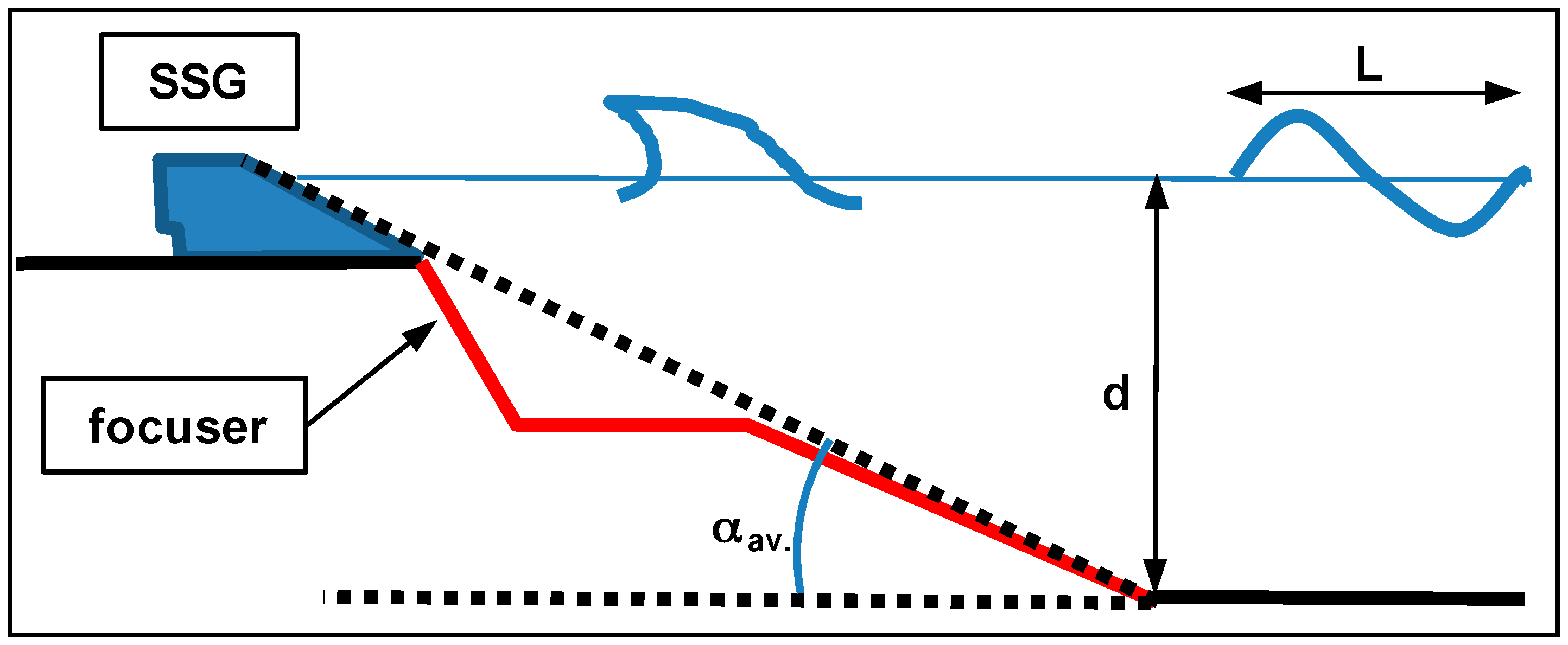
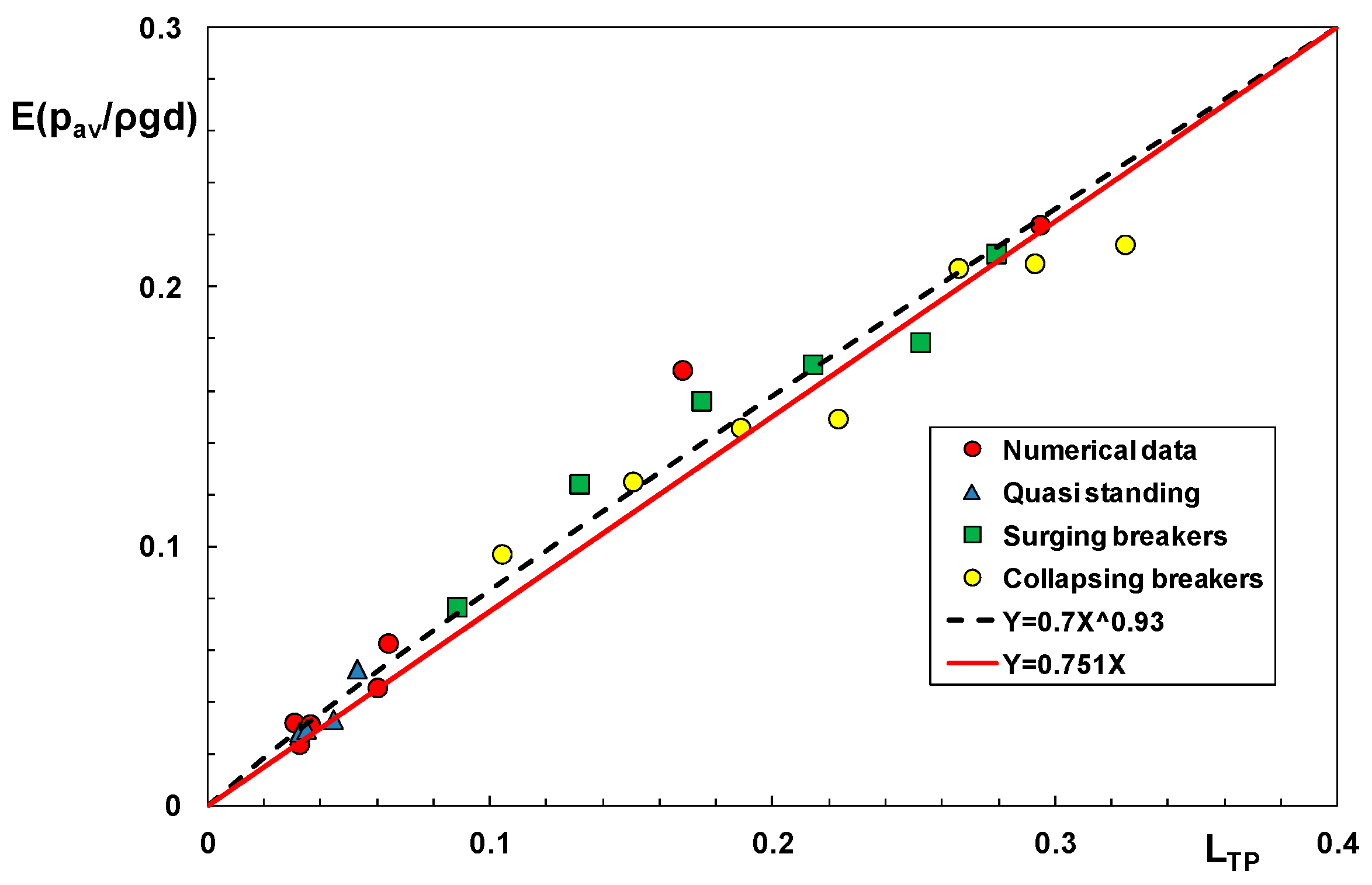
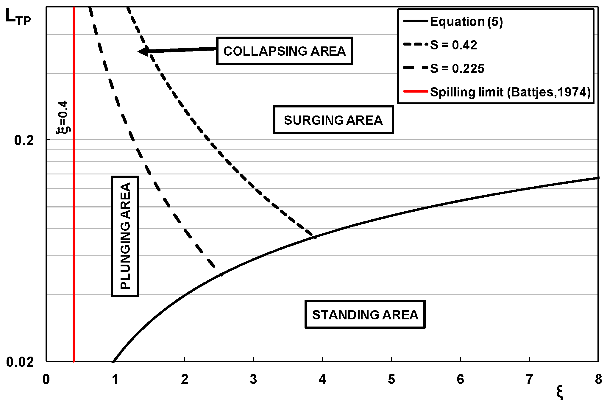
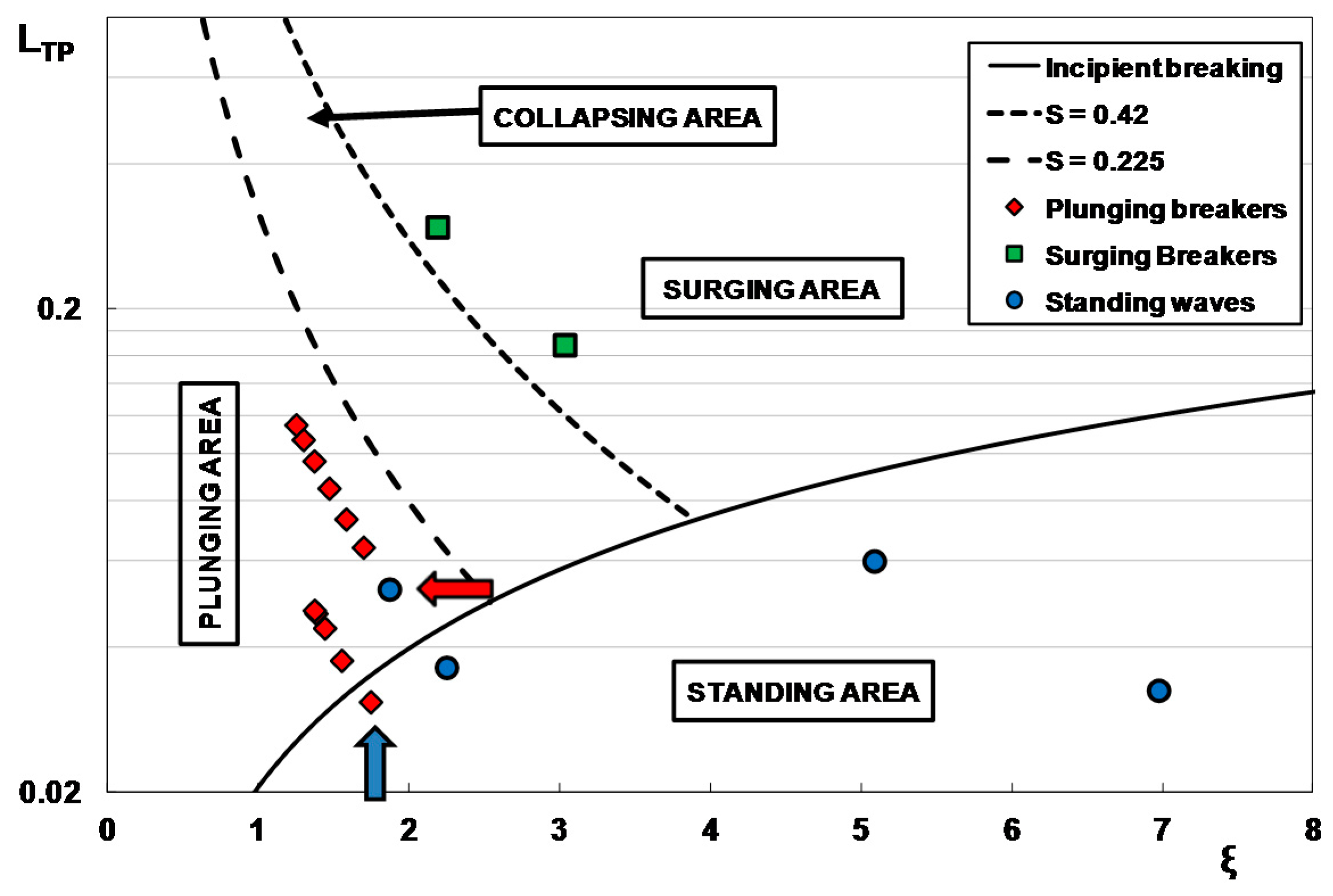
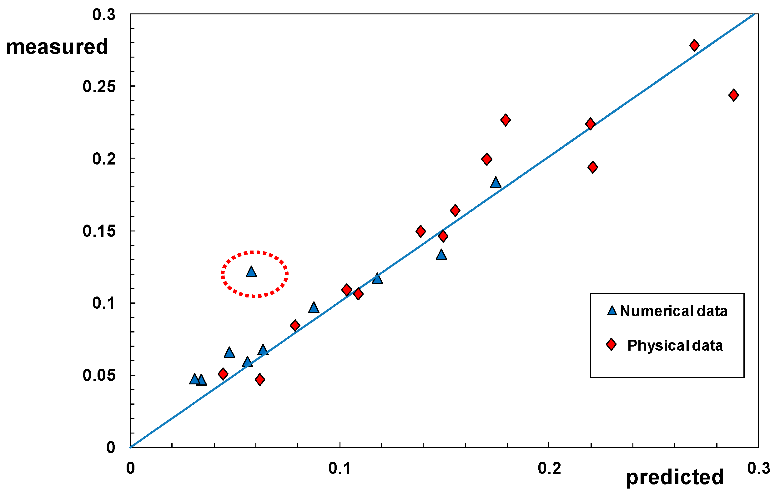
- The Linear Thrust Parameter, which represents the ratio between the maximum value (over a wave period) of the wave momentum flux through the base of the focuser and the corresponding hydrostatic still water thrust:
3. Numerical Experiments
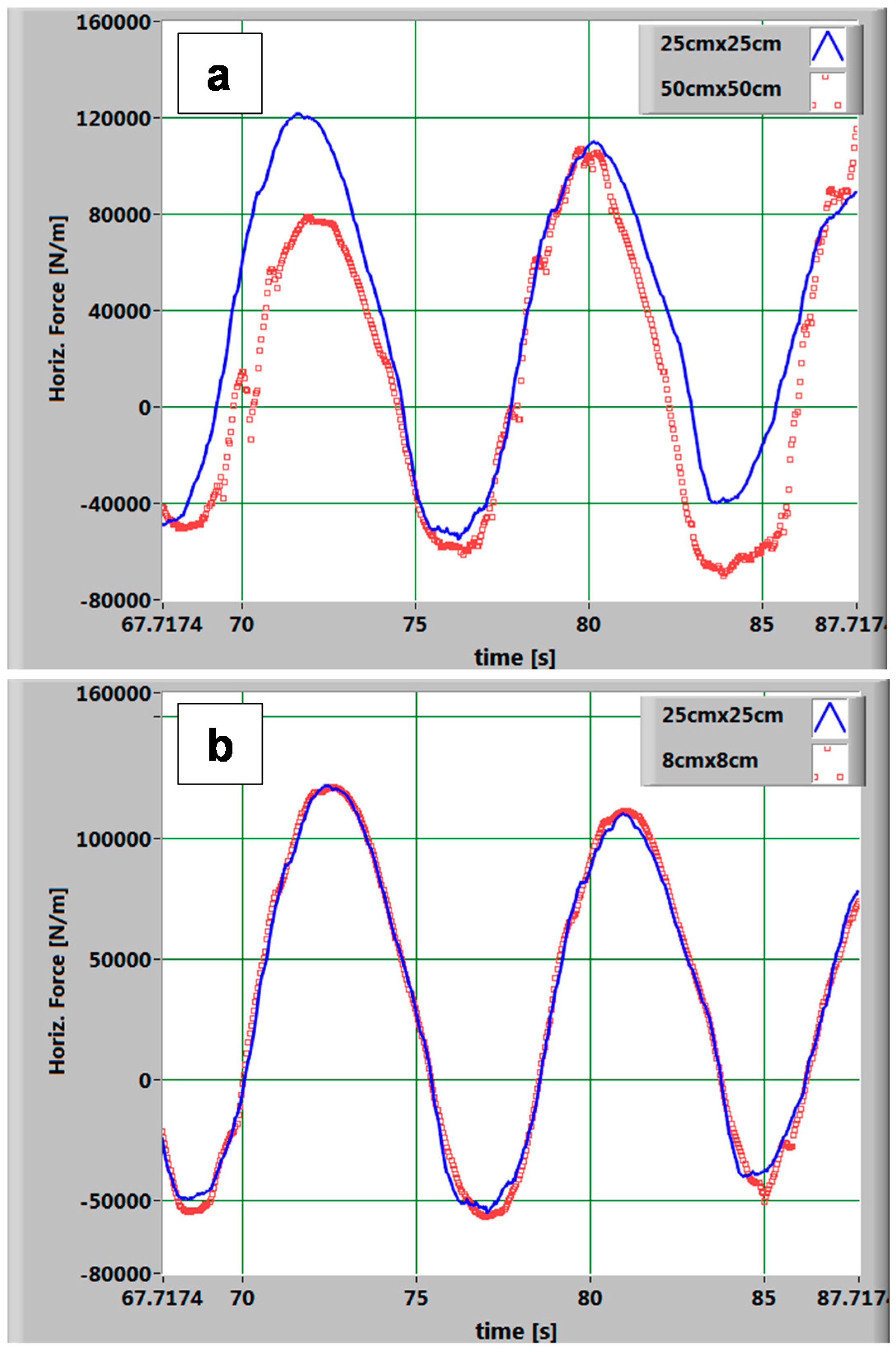
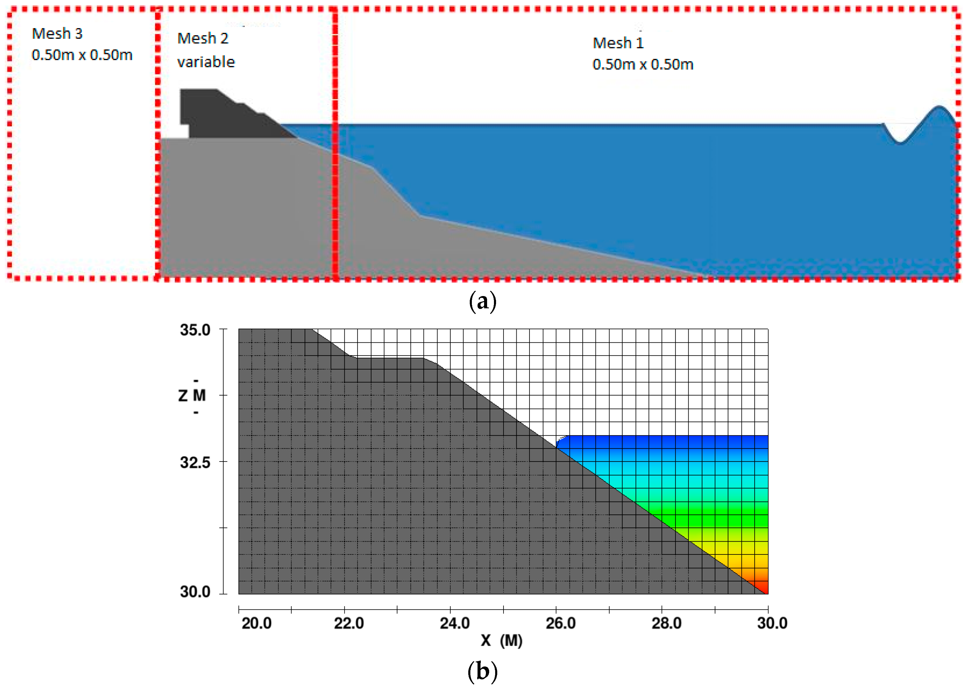
3.1. Grid Selection
3.2. Test Program
3.3. Data
4. Comparison between Results of Numerical and Physical Model Tests
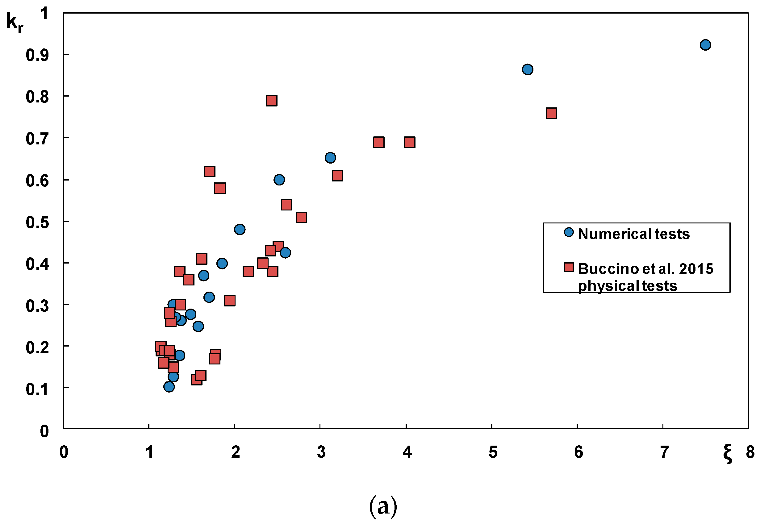
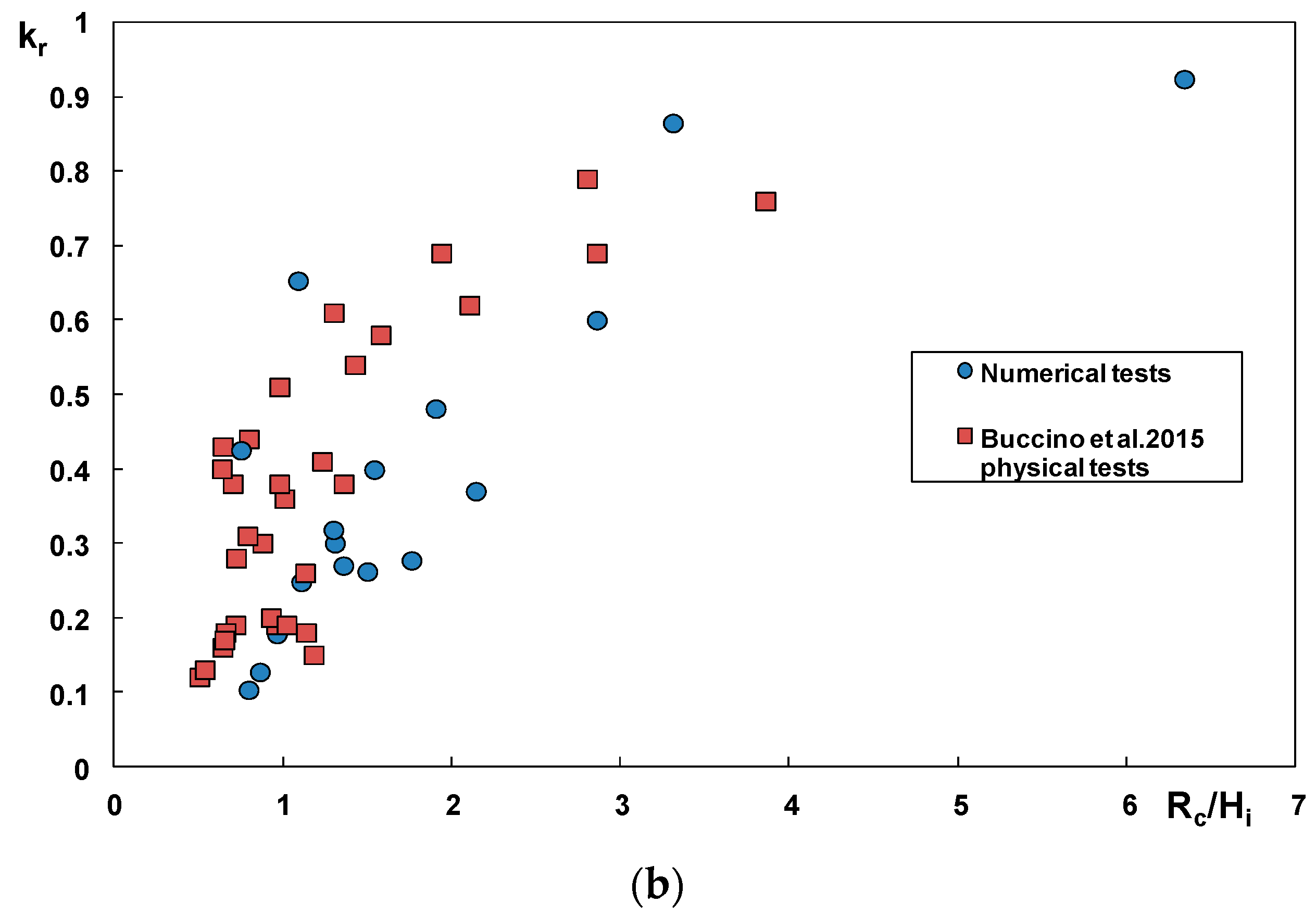
4.1. The Reflection Coefficient
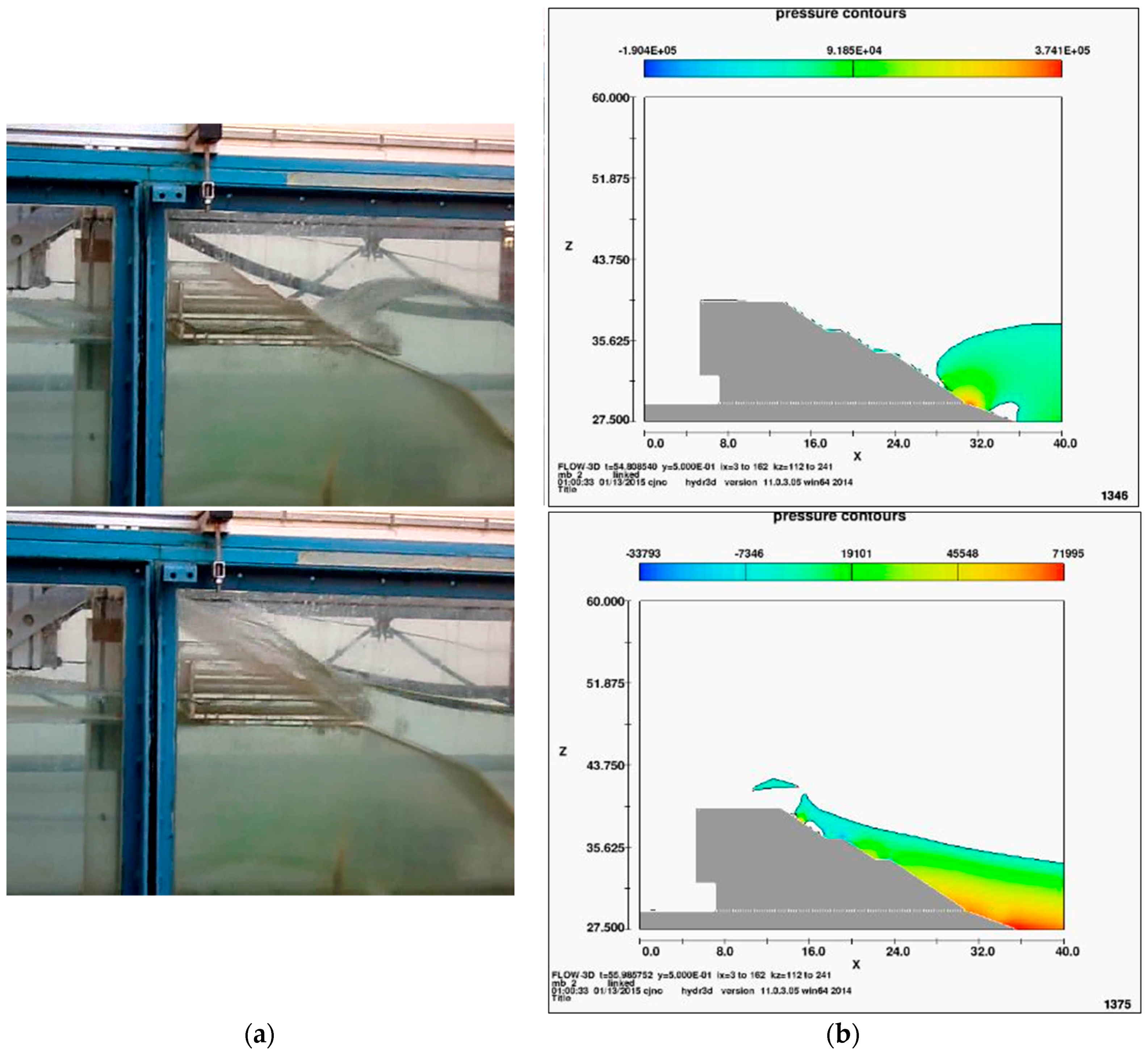
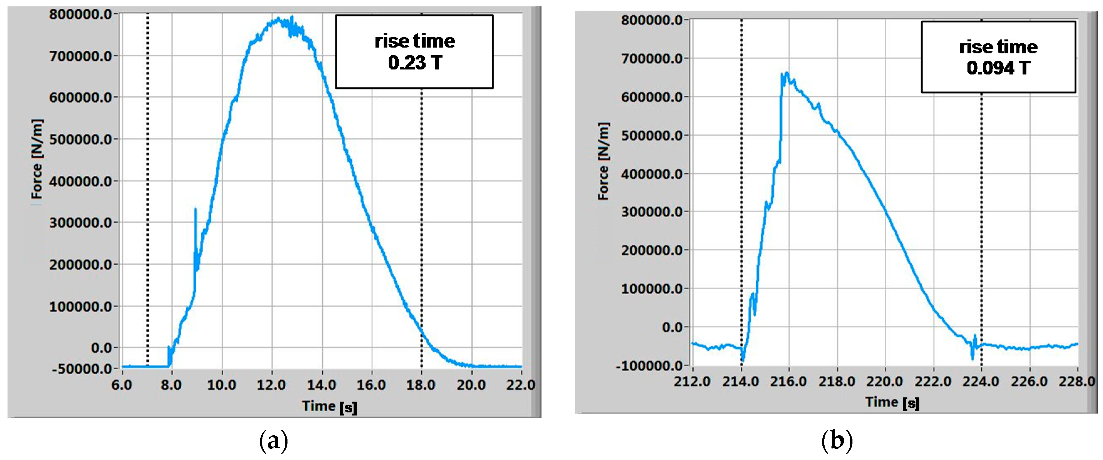
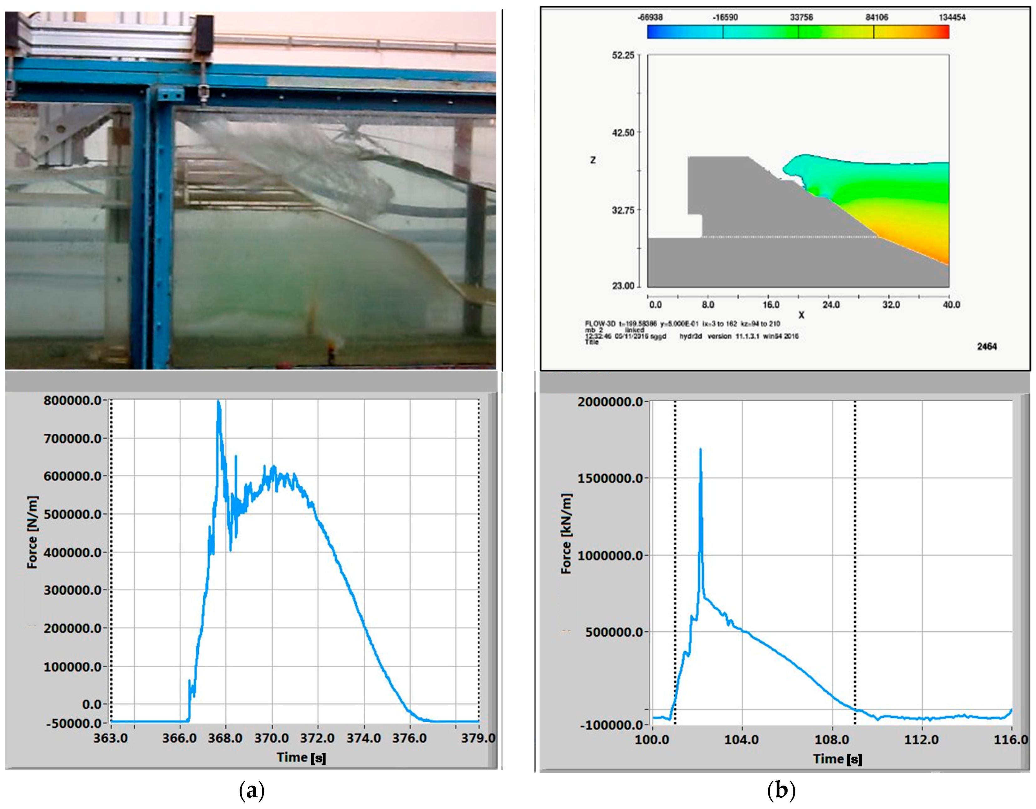
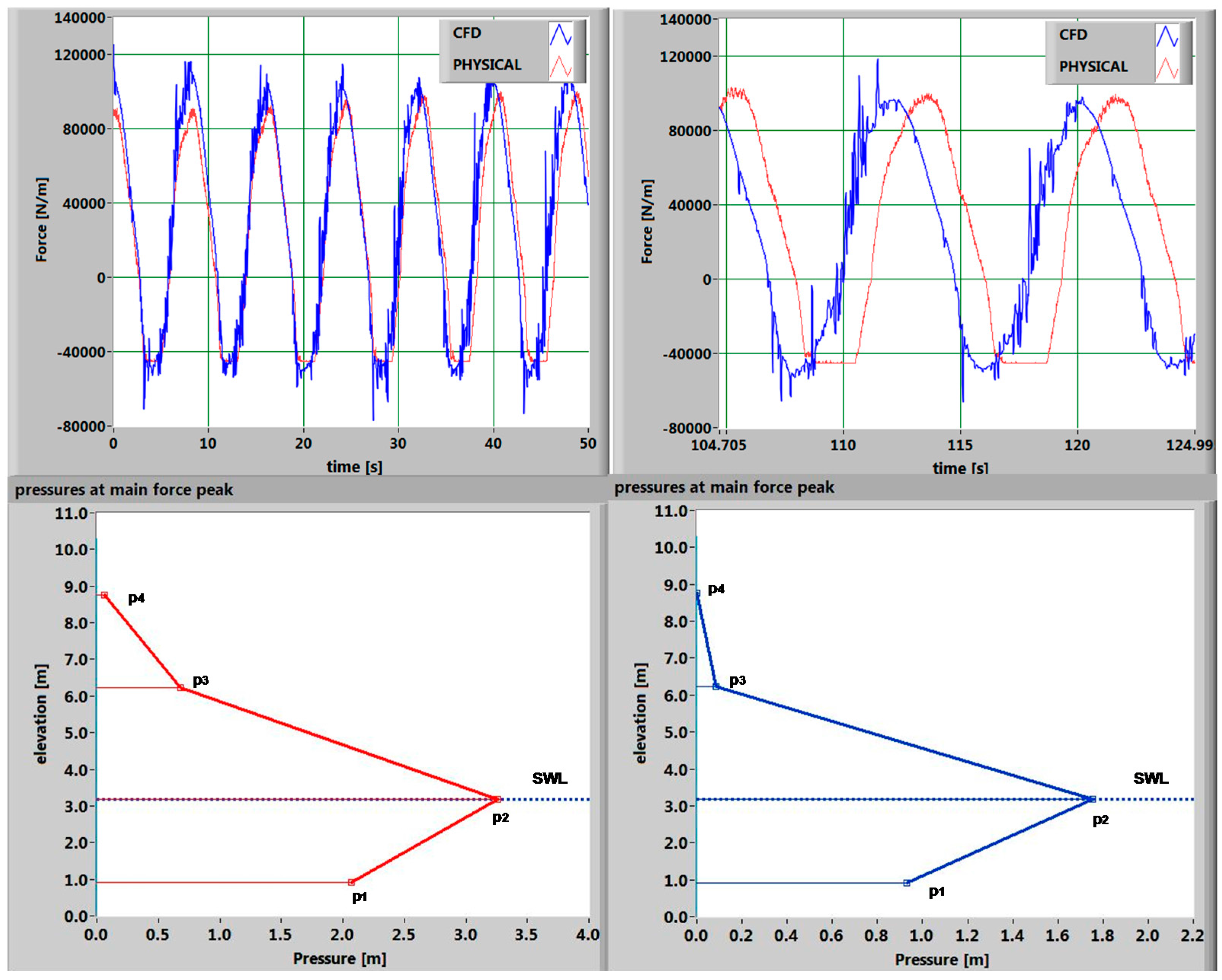
4.2. Wave Shapes at the Wall
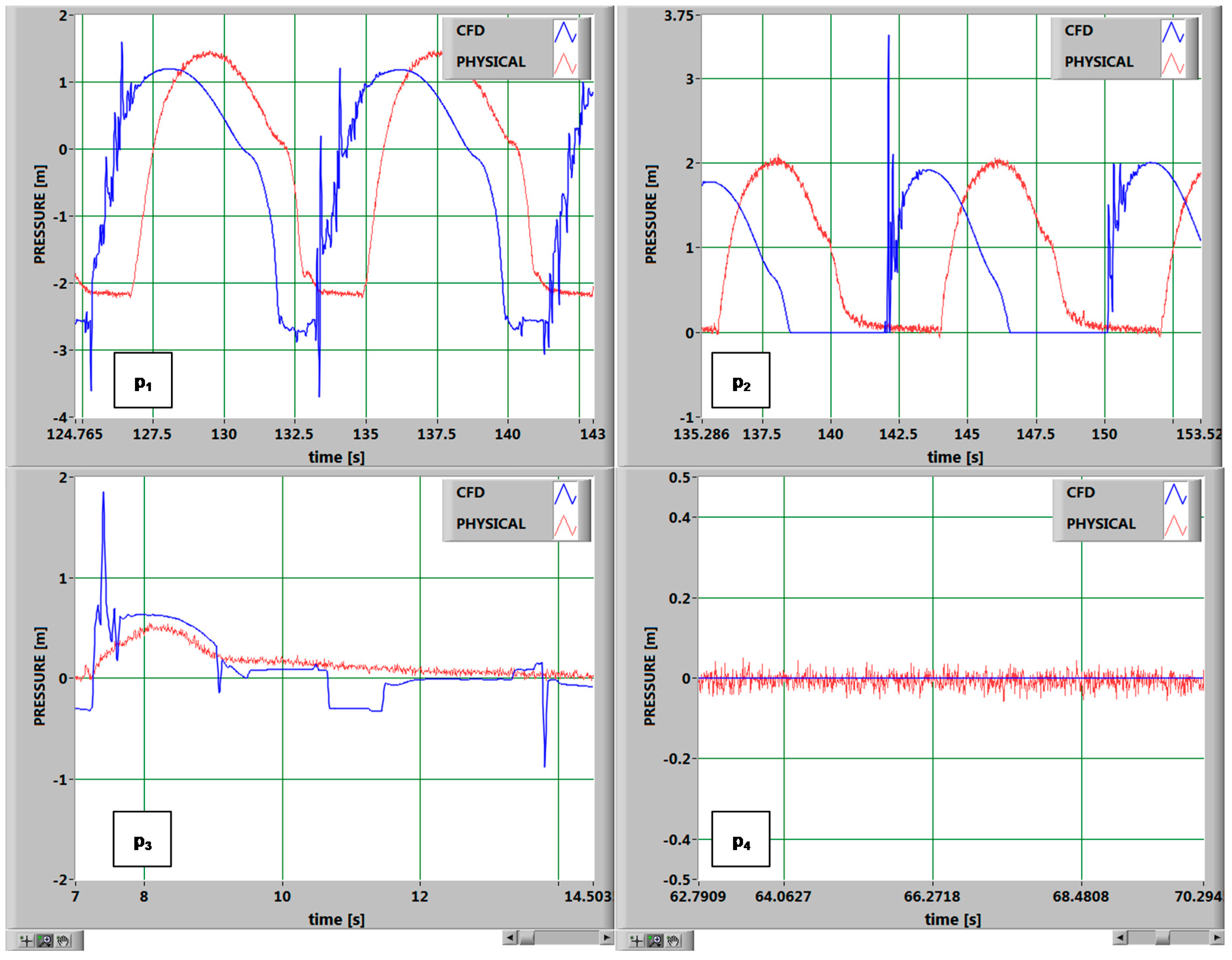
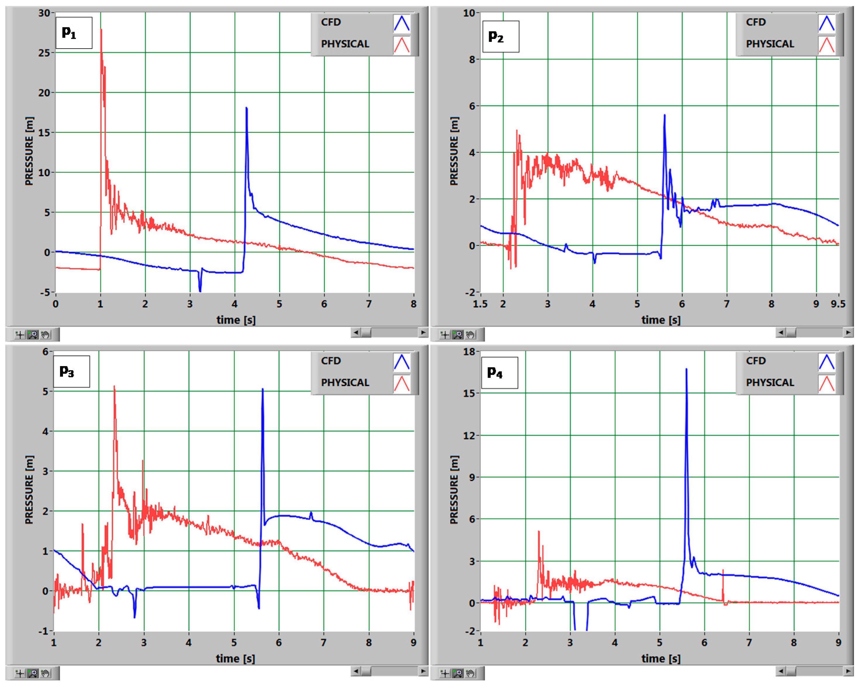
4.3. Direct Comparison of Pressure and Force Signals
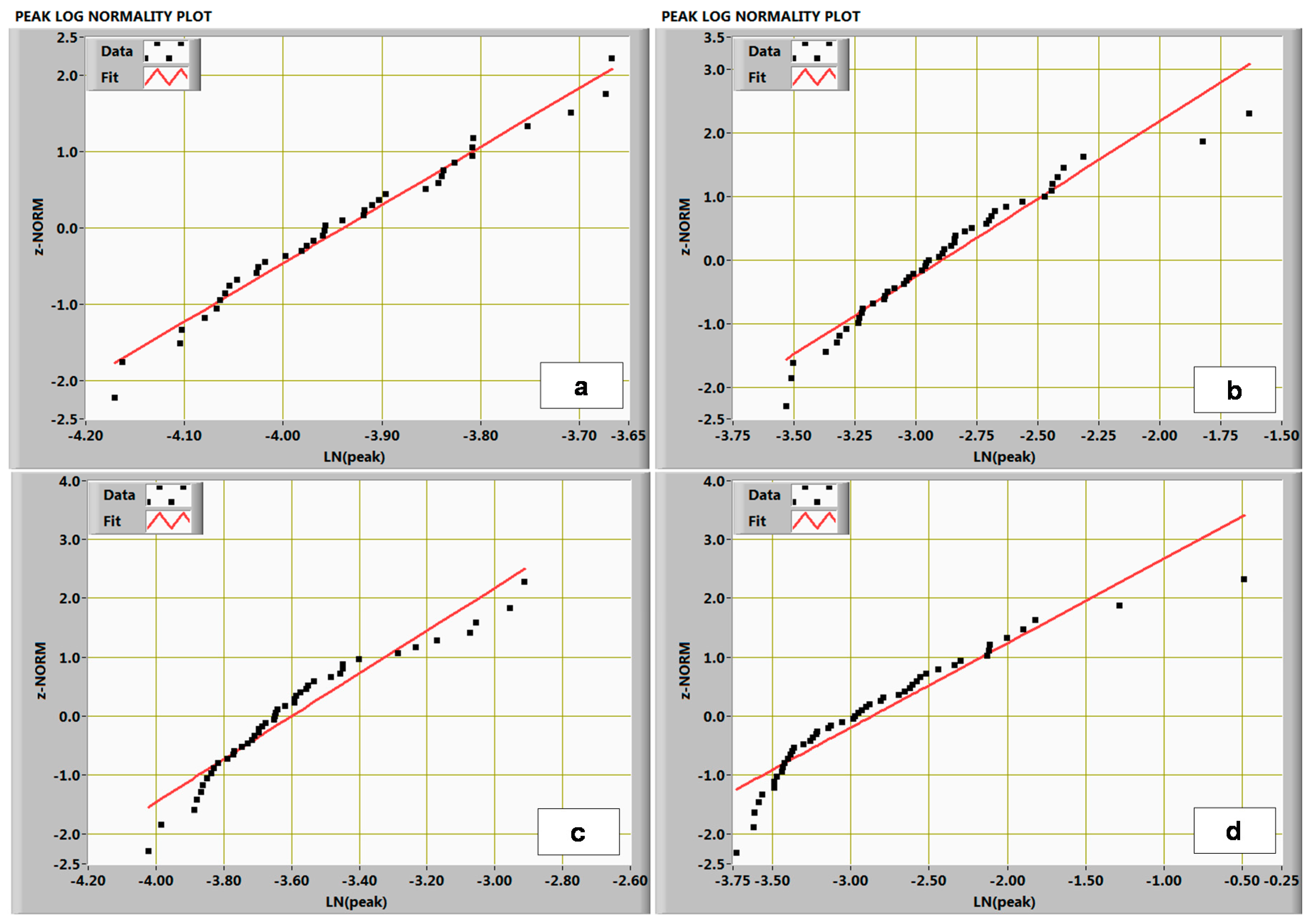
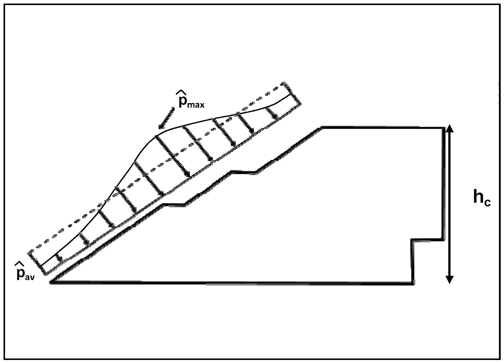
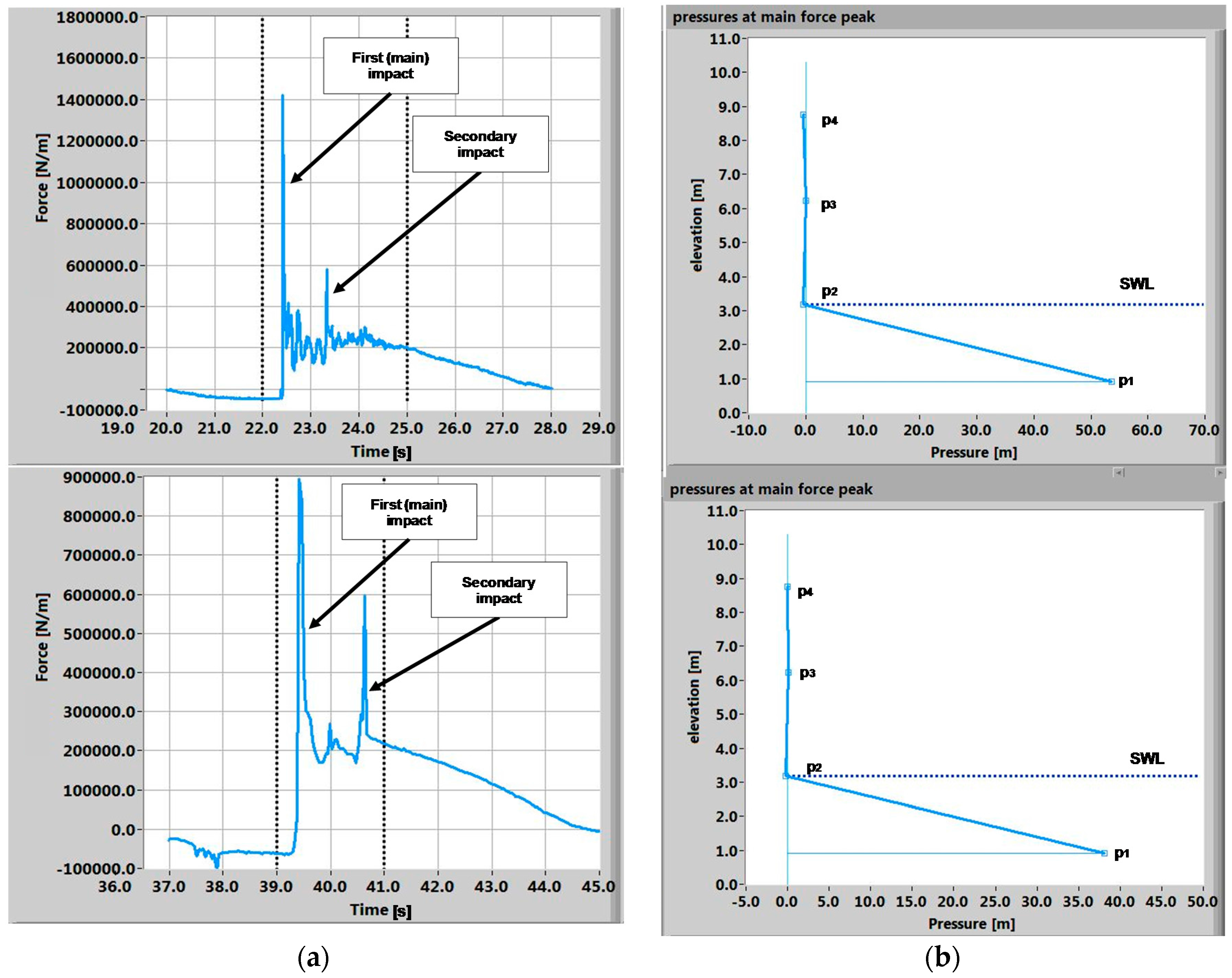
4.4. Wave Loadings Magnitude and Distribution
5. Conclusions
- A weak tendency of CFD at progressively increasing in time the phase difference relative to the physical model (Figure 15 upper panels).
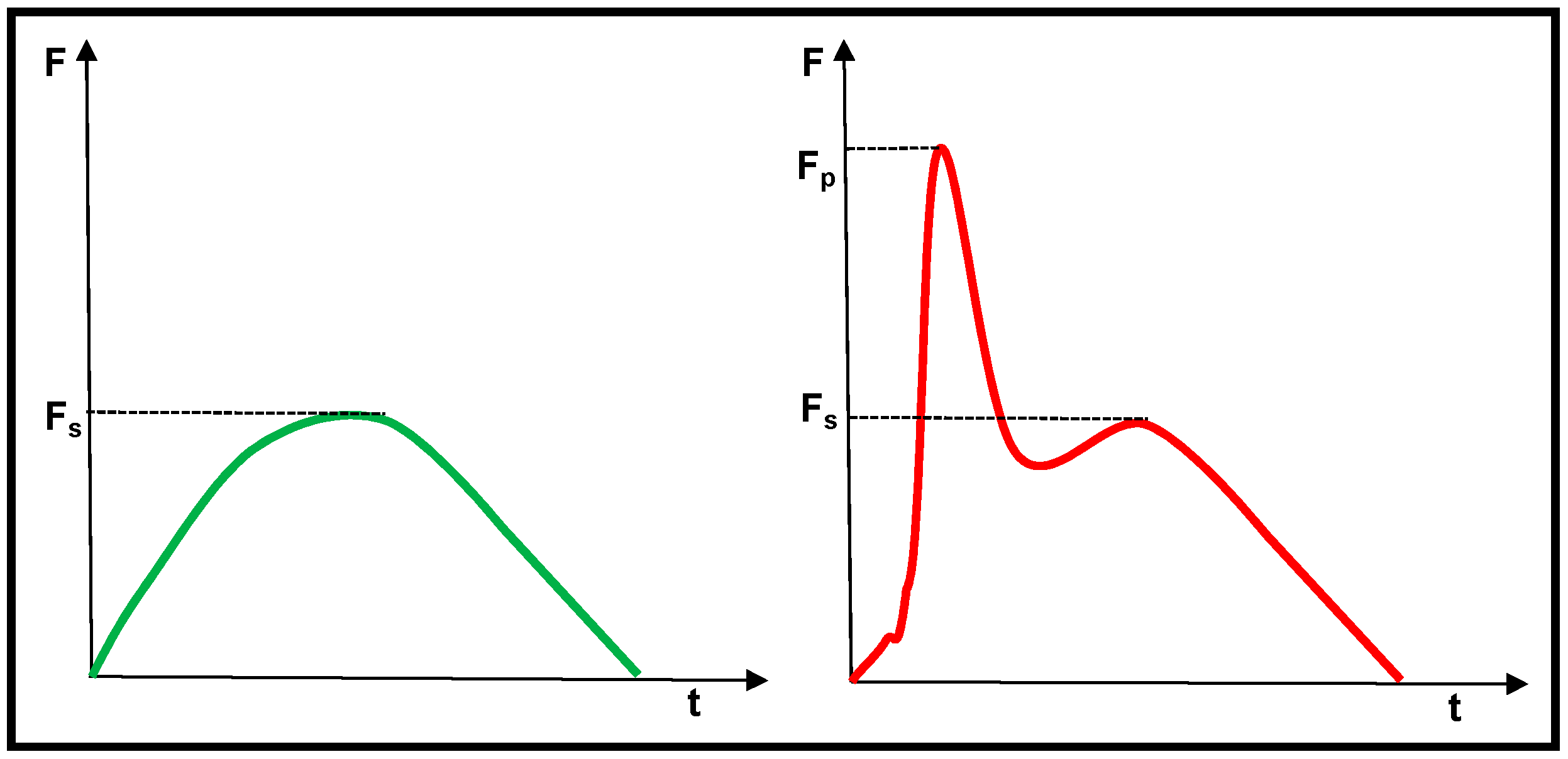
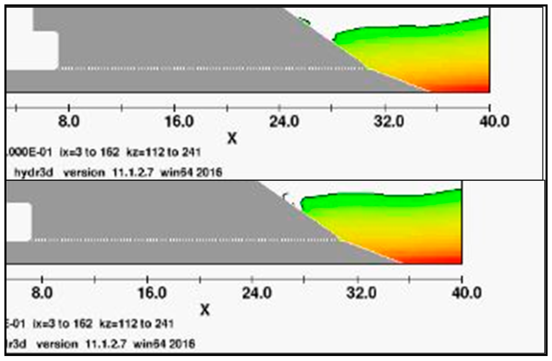
- The presence in the numerical tests of impact events generated by large surging breakers (Figure 19), due to the not modeling of the air that dampens the force peaks in the physical experiments.
Author Contributions
Conflicts of Interest
References
- Frankfurt School FS—UNEP Collaborating Centre for Climate and Sustainable Energy Finance. Global Trend in Renewable Energy Investment; FS-UNEP Publishing: Frankfurt, Germany, 2016. [Google Scholar]
- Clement, A.; McCullen, P.; Falcao, A.; Fiorentino, A.; Gardner, F.; Hammarlund, K.; Lemonis, G.; Lewis, T.; Nielsen, K.; Petroncini, S.; et al. Wave energy in Europe: Current status and perspectives. Renew. Sustain. Energy Rev. 2002, 6, 405–431. [Google Scholar] [CrossRef]
- Azzellino, A.; Conley, D.; Vicinanza, D.; Kofoed, J.P. WECs will likely become diffuse in the near future, thus impacting the further transformation of coastal zones. Marine Renewable Energies: Perspectives and Implications for Marine Ecosystems. Sci. World J. 2013, 2013, 85–88. [Google Scholar]
- Falnes, J. (Ed.) Ocean Wave Energy; Cambridge University Press: Cambridge, UK, 2002.
- Buccino, M.; Vicinanza, D.; Stagonas, D.; Muller, G. Development of a composite seawall wave energy conversion system. Renew. Energy 2015, 81, 509–522. [Google Scholar] [CrossRef] [Green Version]
- Zhang, X.T.; Yang, J.M.; Xiao, L.F. An oscillating wave energy converter with nonlinear snap-through Power-Take-Off systems in waves regular. Chin. Ocean Eng. 2016, 30, 565–580. [Google Scholar] [CrossRef]
- Zhang, X.T.; Yang, J.M. Power capture performance of an oscillating-body WEC with nonlinear snap through PTO systems in irregular waves. Appl. Ocean Res. 2016, 52, 261–273. [Google Scholar] [CrossRef]
- Kofoed, J.P.; Bingham, H.; Christensen, E.D.; Zanuttigh, B.; Martinelli, L.; Castagnetti, M.; Bard, J.; Kracht, P.; Frigaard, P.; Nielsen, K.; et al. State of the Art Descriptions and Tasks for Structural Design of Wave Energy Devices; Department of Civil Engineering, Aalborg University: Aalborg, Denmark, 2010. [Google Scholar]
- GEOwave Consortium. Available online: http//www.geowave-r4sme.eu (accessed on 1 September 2016).
- Vicinanza, D.; Contestabile, P.; Harck Nørgaard, J.Q.; Lykke Andersen, T. Innovative rubble mound breakwaters for overtopping wave energy conversion. Coast. Eng. 2014, 88, 154–170. [Google Scholar] [CrossRef]
- Elhanafi, A. Prediction of regular wave loads on a fixed offshore oscillating water column–wave energy converter using CFD. J. Ocean Eng. Sci. 2016. [Google Scholar] [CrossRef]
- Margheritini, L.; Vicinanza, D.; Frigaard, P. SSG wave energy converter: Design, reliability and hydraulic performance of an innovative overtopping device. J. Renew. Energy 2009, 34, 1371–1380. [Google Scholar] [CrossRef]
- Vicinanza, D.; Margheritini, L.; Kofoed, J.P.; Buccino, M. The SSG wave energy converter: Performance, status and recent developments. Energies 2012, 5, 193–226. [Google Scholar] [CrossRef]
- Buccino, M.; Banfi, D.; Vicinanza, D.; Calabrese, M.D.; Giudice, G.; Carravetta, A. Non breaking wave forces at the front face of Seawave Slotcone Generators. Energies 2012, 5, 4779–4803. [Google Scholar] [CrossRef]
- Buccino, M.; Vicinanza, D.; Salerno, D.; Banfi, D.; Calabrese, M. Nature and magnitude of wave loadings at Seawave Slot-cone Generators. Ocean Eng. 2015, 95, 34–58. [Google Scholar] [CrossRef]
- Vicinanza, D.; Frigaard, P. Wave pressure acting on a seawave slot-cone generator. Coast. Eng. 2009, 55, 553–568. [Google Scholar] [CrossRef]
- Takahashi, S.; Hosoyamada, S.; Yamamoto, S. Hydrodynamic characteristics of sloping top caissons. In Proceedings of the International Conference on HydroTechnical Engineering for Port and Harbor Construction, 1. Port and Harbour, Yokosuka, Japan, 19–21 October 1994; Port and Harbour Research Institute: Tokyo, Japan, 1994; pp. 733–746. [Google Scholar]
- Vicinanza, D.; Ciardulli, F.; Buccino, M.; Calabrese, M.; Kofoed, J.P. Wave loadings acting on an innovative breakwater for energy production. J. Coast. Res. 2011, 64, 608–612. [Google Scholar]
- Tanimoto, K.; Kimura, K. A hydraulic Experiment Study on Trapezoidal Caisson Breakwaters; Port and Harbour Research Institute: Yokosuka, Japan, 1985. [Google Scholar]
- Battjes, J.A. Surf similarity. In Proceedings of the 14th Coastal Engineering Conference, Copenhagen, Denmark, 24–28 June 1974.
- Svendsen, I.B.A. Introduction to Nearshore Hydrodynamics; World Scientific: Singapore, 2006. [Google Scholar]
- Hughes, S.A. Wave momentum flux parameter: A descriptor for nearshore waves. Coast. Eng. 2004, 51, 1067–1084. [Google Scholar] [CrossRef]
- Calabrese, M.; Vicinanza, D.; Buccino, M. 2D wave setup behind low crested and submerged breakwaters. In Proceedings of the 13th International Offshore and Polar Engineering Conference, Honolulu, HI, USA, 25–30 May 2003.
- Calabrese, M.; Buccino, M.; Pasanisi, M. Wave breaking macrofeatures on a submerged rubble mound break water. J. Hydro-Environ. Res. 2008, 1, 216–225. [Google Scholar] [CrossRef]
- Oumeraci, H.; Allsop, N.W.H.; De Groot, M.B.; Crouch, R.S.; Vrijling, J.K. Probabilistic Design Tools for Vertical Breakwaters; Balkema: Rotterdam, The Netherlands, 1999. [Google Scholar]
- Peregrine, D.H. Water wave impact on walls. Ann. Rev. Fluid Mech. 2003, 35, 23–44. [Google Scholar] [CrossRef]
- Calabrese, M.; Buccino, M. Wave Impacts on vertical and composite breakwaters. In Proceedings of the 10th International Offshore and Polar Engineering Conference, Seattle, WA, USA, 28 May–2 June 2000.
- Flow Science Inc. Suite Flow 3D; Flow Science Inc.: Santa Fe, Mexico, 2009. [Google Scholar]
- Dentale, F.; Donnarumma, G.; Pugliese Carratelli, E. Simulation of flow within armour blocks in a breakwater. J. Coast. Res. 2014, 30, 528–536. [Google Scholar] [CrossRef]
- Dentale, F.; Donnarumma, G.; Pugliese Carratelli, E. Numerical wave interaction with Tetrapods breakwater. J. Naval Arch. Ocean Eng. 2014, 6, 800–812. [Google Scholar] [CrossRef]
- Kortenhaus, A.; van der Meer, J.W.; Burcharth, H.F.; Geeraerts, J.; van Gent, M.; Pullen, T. Final Report on Scale Effects; CLASH WP7-Report; LWI: Braunschweig, Germany, 2004. [Google Scholar]
- Zanuttigh, B.; Margheritini, L.; Gambles, L.; Martinelli, L. Analysis of wave reflection from Wave Energy Converters installed as breakwaters in harbors. In Proceedings of the European Wave and Tidal Energy Conference (EWTEC), Uppsala, Sweden, 7–10 September 2009.
- Zelt, J.A.; Skjelbreia, J.E. Estimating incident and reflected wave field using an arbitrary number of wave gauges. In Proceedings of the International Conference on Coastal Engineering, Venice, Italy, 4–9 October 1992; pp. 777–789.
- Basco, D. A qualitative description of wave breaking. J. Waterw. Port Coast. Ocean Eng. 1985, 111, 171–188. [Google Scholar] [CrossRef]
- Goda, Y. Random Seas and Design of Maritime Structures; World Scientific: Singapore, 2010. [Google Scholar]


| GRID | RMSE | R2 |
|---|---|---|
| 50 × 50 vs. 25 × 25 | 6.36 | 0.86 |
| 25 × 25 vs. 8 × 8 | 0.37 | 0.99 |
| TEST# | Hi [m] | T [s] | Δt* [s] |
|---|---|---|---|
| 1 | 3.01 | 6.70 | 0.03 |
| 2 | 3.73 | 6.64 | 0.03 |
| 3 | 4.34 | 6.65 | 0.03 |
| 4 | 4.68 | 6.63 | 0.03 |
| 5 | 4.75 | 6.63 | 0.03 |
| 6 | 2.61 | 8.01 | 0.04 |
| 7 | 3.78 | 8.02 | 0.04 |
| 8 | 4.58 | 8.04 | 0.04 |
| 9 | 5.25 | 8.03 | 0.04 |
| 10 | 6.08 | 8.03 | 0.04 |
| 11 | 6.95 | 8.01 | 0.04 |
| 12 | 7.71 | 8.00 | 0.04 |
| 13 | 8.29 | 7.99 | 0.04 |
| 14 | 1.25 | 17.15 | 0.08 |
| 15 | 2.32 | 17.05 | 0.08 |
| 16 | 6.50 | 17.03 | 0.08 |
| 17 | 11.55 | 16.40 | 0.08 |
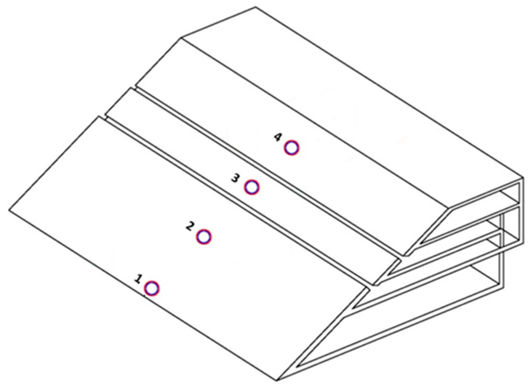
| Transducer# | Transducer Centre from the SSG Toe [m] |
|---|---|
| 1 | 0.93 |
| 2 | 3.70 |
| 3 | 6.24 |
| 4 | 8.75 |
| TEST# | CFD | PHYSICAL | ERR (%) | BREAKER TYPE | ||||
|---|---|---|---|---|---|---|---|---|
| Hi [m] | T [s] | Hi [m] | T [s] | Hi | T | Physical | Numerical | |
| A | 2.61 | 8.01 | 2.37 | 8.12 | 10 | 1 | Standing | Standing |
| B | 7.71 | 8.00 | 7.62 | 8.12 | 1 | 2 | Plunging | Plunging |
| C | 11.55 | 16.40 | 10.70 | 16.33 | 8 | 0 | Surging | Surging |
© 2016 by the authors; licensee MDPI, Basel, Switzerland. This article is an open access article distributed under the terms and conditions of the Creative Commons Attribution (CC-BY) license (http://creativecommons.org/licenses/by/4.0/).
Share and Cite
Buccino, M.; Dentale, F.; Salerno, D.; Contestabile, P.; Calabrese, M. The Use of CFD in the Analysis of Wave Loadings Acting on Seawave Slot-Cone Generators. Sustainability 2016, 8, 1255. https://doi.org/10.3390/su8121255
Buccino M, Dentale F, Salerno D, Contestabile P, Calabrese M. The Use of CFD in the Analysis of Wave Loadings Acting on Seawave Slot-Cone Generators. Sustainability. 2016; 8(12):1255. https://doi.org/10.3390/su8121255
Chicago/Turabian StyleBuccino, Mariano, Fabio Dentale, Daniela Salerno, Pasquale Contestabile, and Mario Calabrese. 2016. "The Use of CFD in the Analysis of Wave Loadings Acting on Seawave Slot-Cone Generators" Sustainability 8, no. 12: 1255. https://doi.org/10.3390/su8121255