
An RVM-Based Model for Assessing the Failure Probability of Slopes along the Jinsha River, Close to the Wudongde Dam Site, China

Abstract
:1. Introduction
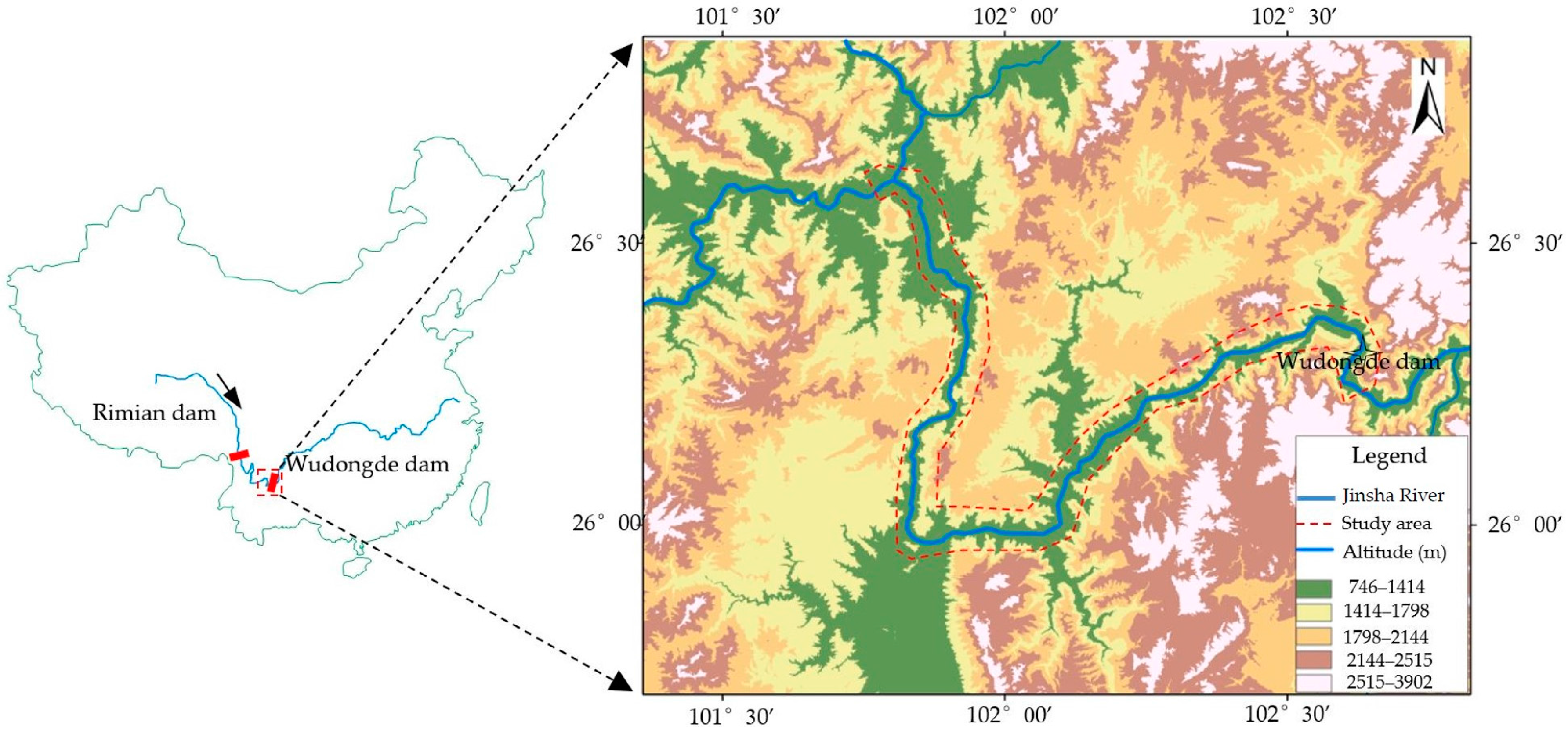
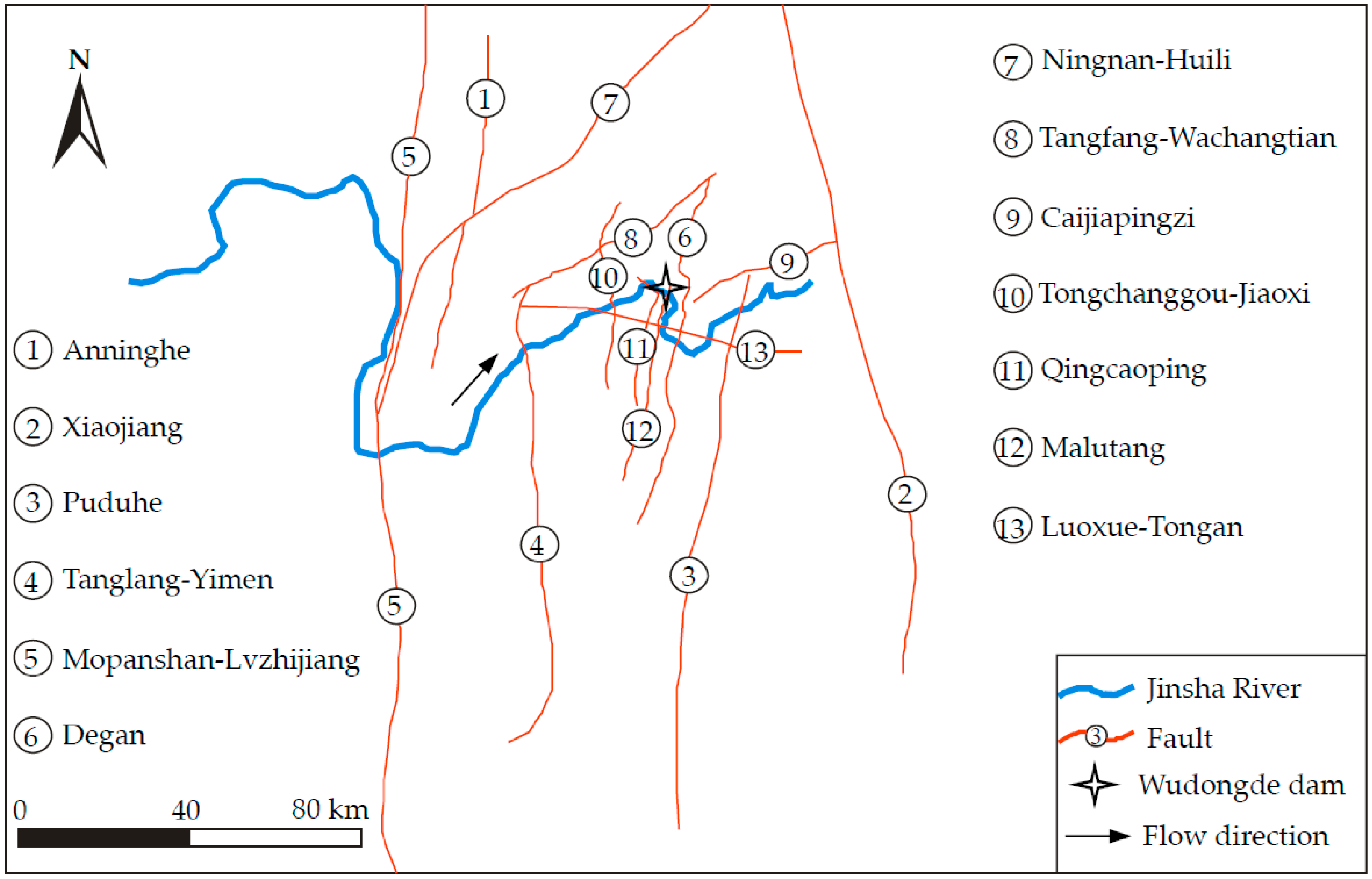
2. Study Area
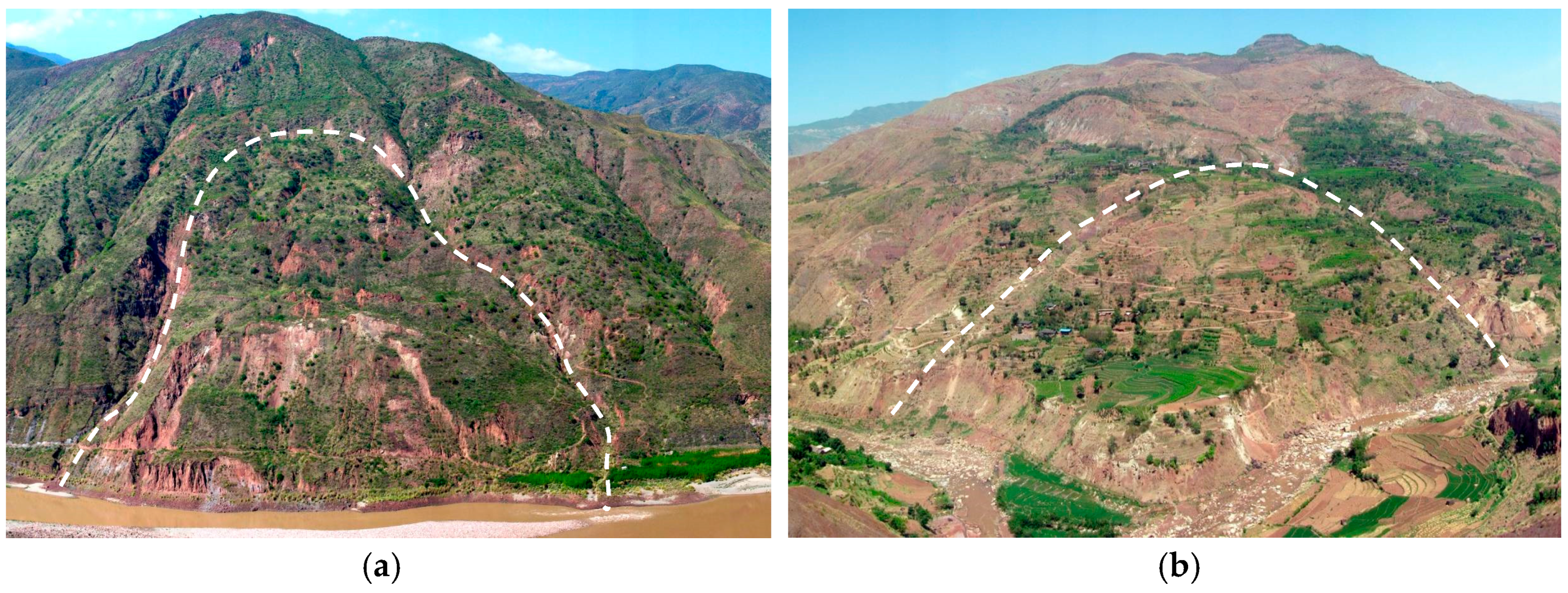
2.1. Geological and Geomorphological Settings
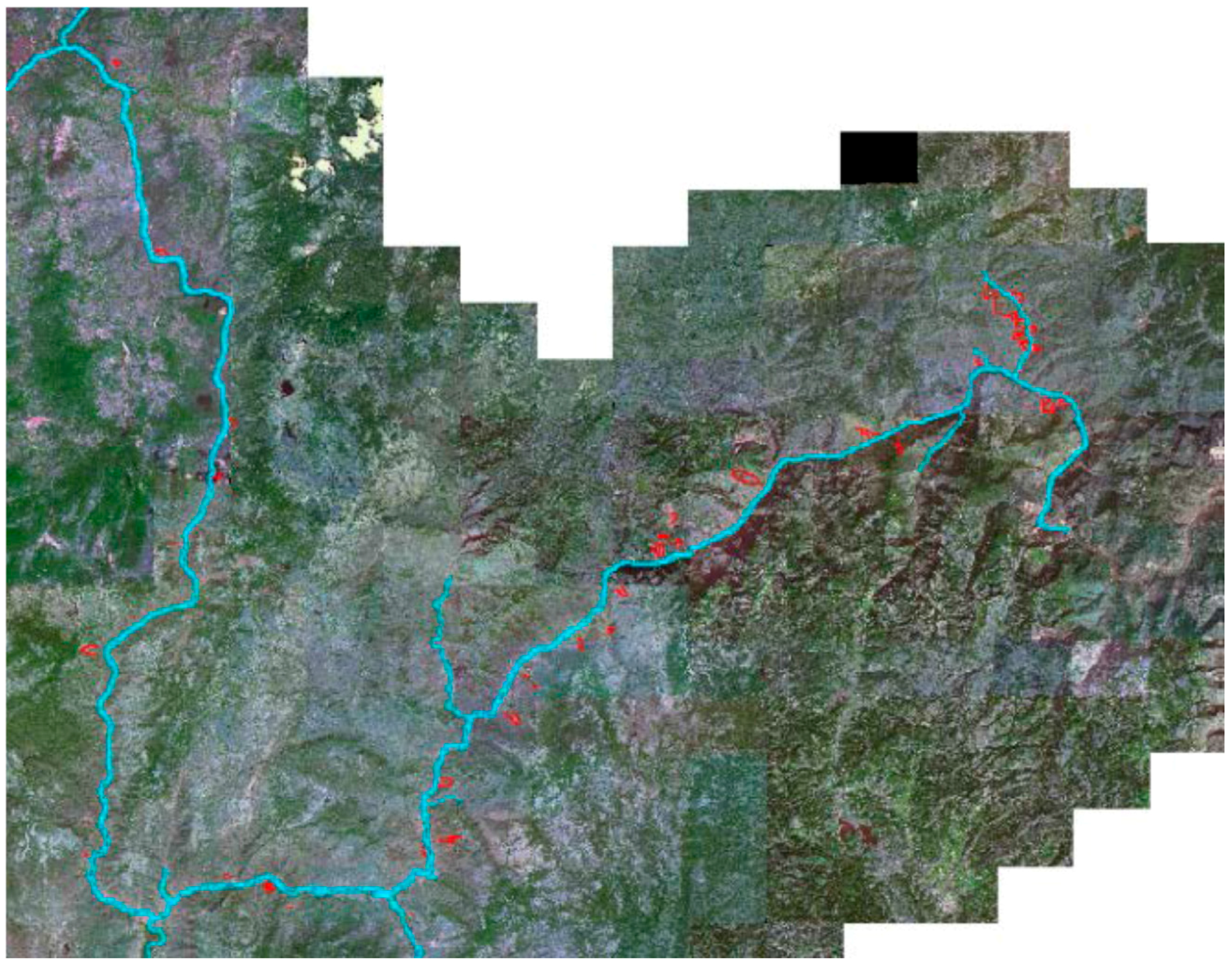
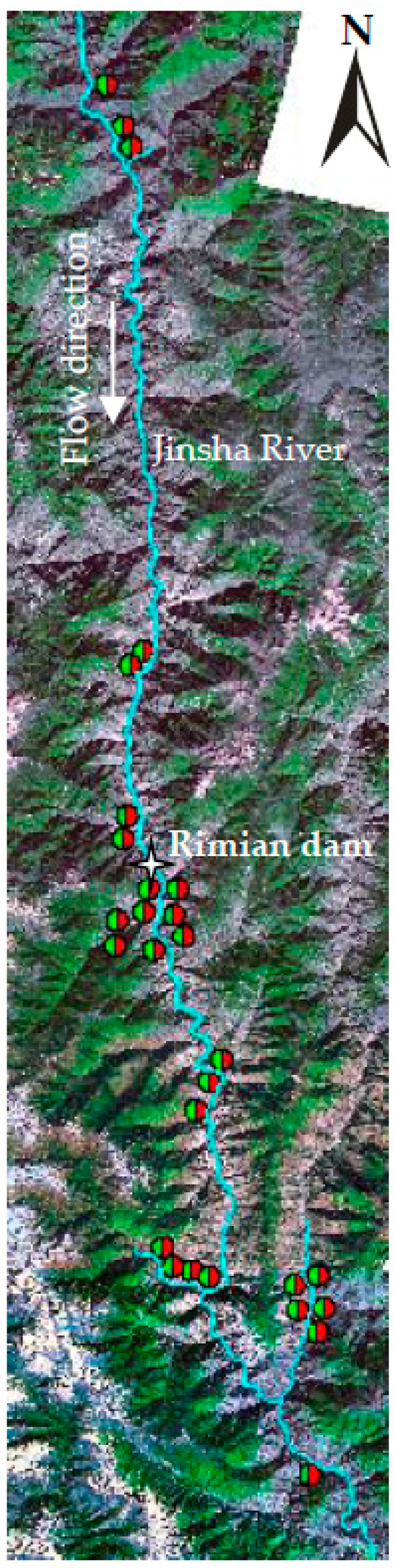
2.2. Landslide Identification
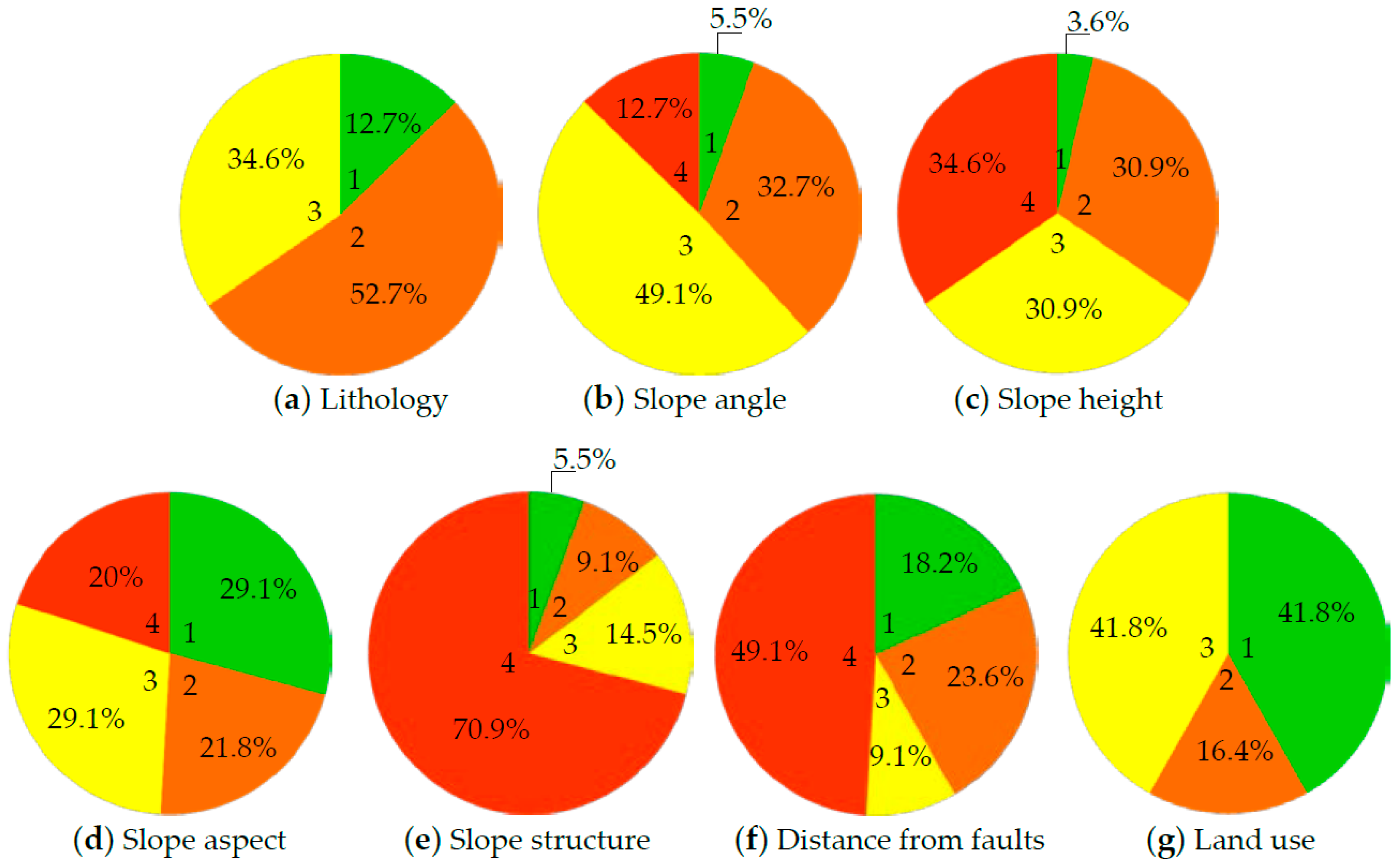
3. Influencing Factors
3.1. Lithology
3.2. Slope Angle
3.3. Slope Height
3.4. Slope Aspect
3.5. Slope Structure
3.6. Distance from Faults
3.7. Land Use
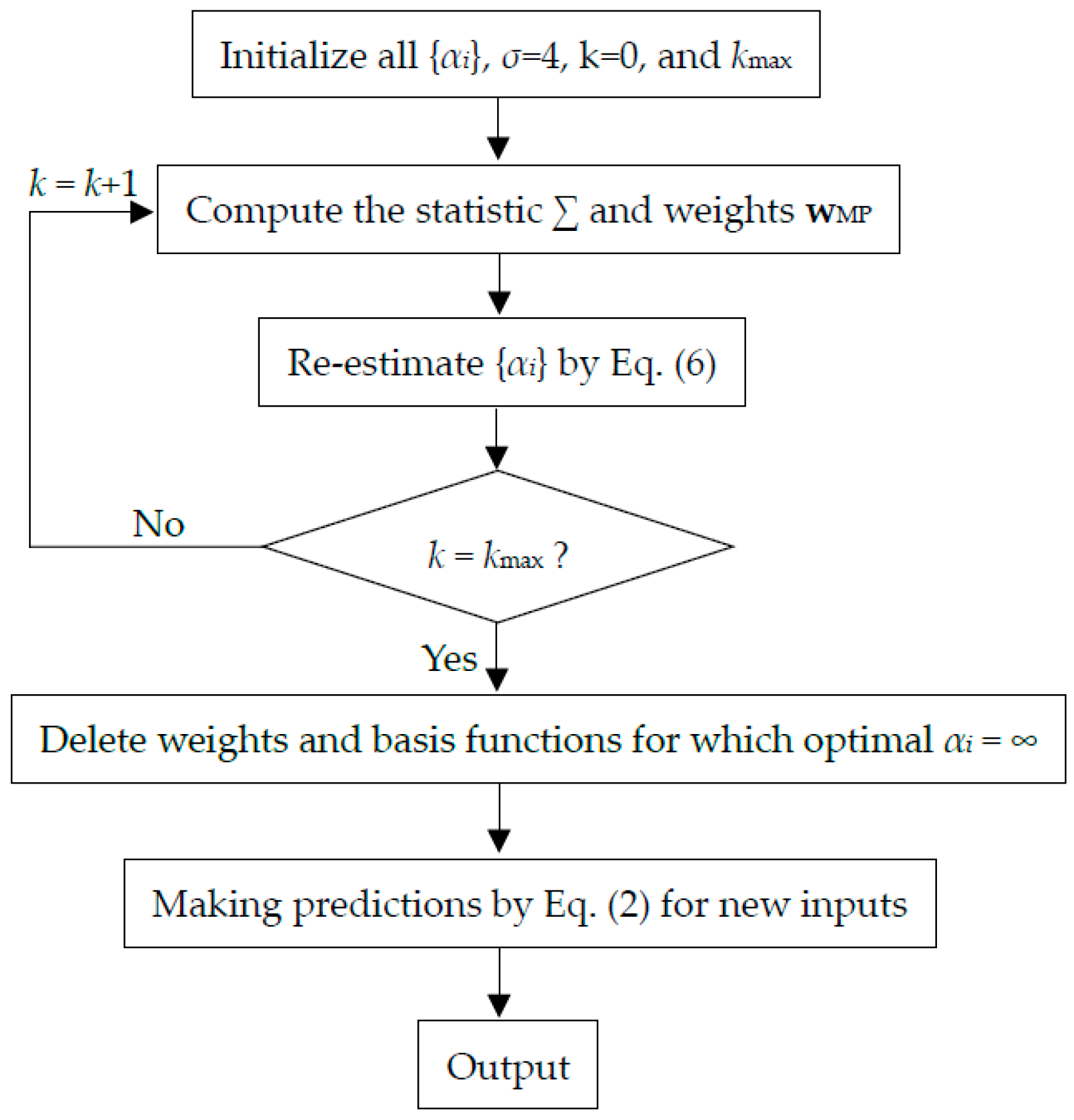
4. Relevance Vector Machine
5. Results and Discussions
5.1. Data Processing
5.2. Preparation of Training and Testing Data
5.3. Parameter Determination
5.4. Training and Testing of the RVM Model
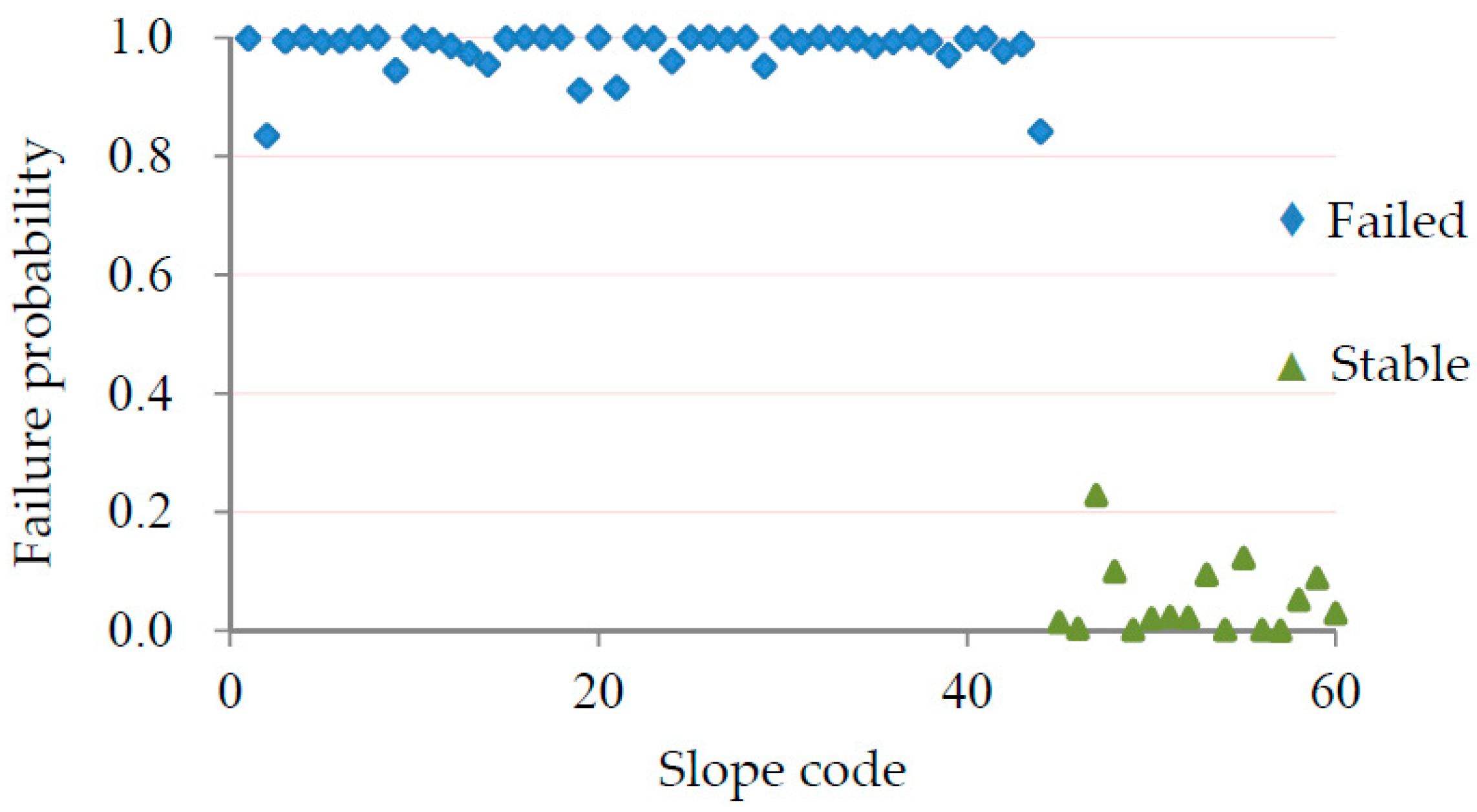
5.5. Evaluation of the Model
6. Conclusions
Acknowledgments
Author Contributions
Conflicts of Interest
References
- Aleotti, P.; Chowdhury, R. Landslide hazard assessment: Summary review and new perspectives. Bull. Eng. Geol. Environ. 1999, 58, 21–44. [Google Scholar] [CrossRef]
- Pappalardo, G.; Mineo, S.; Rapisarda, F. Rockfall hazard assessment along a road on the Peloritani Mountains (northeastern Sicily, Italy). Nat. Hazards Earth Syst. Sci. 2014, 14, 2735–2748. [Google Scholar] [CrossRef] [Green Version]
- Zhou, S.; Chen, G.; Fang, L.; Nie, Y. GIS-Based integration of subjective and objective weighting methods for regional landslides susceptibility mapping. Sustainability 2016, 8, 334. [Google Scholar]
- Carrara, A.; Merenda, L. GIS techniques and statistical models in evaluating landslide hazard. Earth Surf. Proc. Land. 1991, 16, 427–445. [Google Scholar] [CrossRef]
- Saroglou, H.; Marinos, V.; Marinos, P.; Tsiambaos, G. Rockfall hazard and risk assessment: An example from a high promontory at the historical site of Monemvasia, Greece. Nat. Hazards Earth Syst. Sci. 2012, 12, 1823–1836. [Google Scholar] [CrossRef] [Green Version]
- Pradhan, B. A comparative study on the predictive ability of the decision tree, support vector machine and neuro-fuzzy models in landslide susceptibility mapping using GIS. Comput. Geosci. 2013, 51, 350–365. [Google Scholar] [CrossRef] [Green Version]
- Günther, A.; Reichenbach, P.; Malet, J.P.; Van Den Eeckhaut, M.; Hervás, J.; Dashwood, C.; Guzzetti, F. Tier-Based approaches for landslide susceptibility assessment in Europe. Landslides 2012, 10, 529–546. [Google Scholar] [CrossRef] [Green Version]
- Ayalew, L.; Yamagishi, H. The application of GIS-based logistic regression for landslide susceptibility mapping in the Kakuda-Yahiko Mountains, central Japan. Geomorphology 2005, 65, 15–31. [Google Scholar] [CrossRef]
- Manzo, G.; Tofani, V.; Segoni, S.; Battistini, A.; Catani, F. GIS techniques for regional scale landslide susceptibility assessment: The Sicily (Italy) case study. Int. J. Geogr. Inf. Sci. 2013, 27, 1433–1452. [Google Scholar] [CrossRef]
- Liang, W.J.; Zhuang, D.F.; Dong, J.; Pan, J.J.; Ren, H.Y. Assessment of debris flow hazards using a Bayesian Network. Geomorphology 2012, 171–172, 94–100. [Google Scholar] [CrossRef]
- Song, Y.Q.; Gong, J.H.; Gao, S.; Wang, D.C.; Cui, T.J.; Li, Y.; Wei, B.Q. Susceptibility assessment of earthquake-induced landslides using Bayesian network: A case study in Beichuan, China. Comput. Geosci. 2012, 42, 189–199. [Google Scholar] [CrossRef]
- Guzzetti, F.; Reichenbach, P.; Ardizzone, F.; Cardinali, M.; Galli, M. Estimating the quality of landslide susceptibility models. Geomorphology 2006, 81, 166–184. [Google Scholar] [CrossRef]
- Yao, X.; Tham, L.G.; Dai, F.C. Landslide susceptibility mapping based on Support Vector Machine: A case study on natural slopes of Hong Kong, China. Geomorphology 2008, 101, 572–582. [Google Scholar] [CrossRef]
- Lee, S.; Ryu, J.; Won, J.; Park, H. Determination and application of weights for landslide susceptibility mapping using an artificial neural network. Eng. Geol. 2004, 71, 289–302. [Google Scholar] [CrossRef]
- Ermini, L.; Catani, F.; Casagli, N. Artificial neural network to landslide susceptibility assessment. Geomorphology 2005, 66, 327–343. [Google Scholar] [CrossRef]
- Lin, H.M.; Chang, S.H.; Wu, J.H.; Juang, C.H. Neural network-based model for assessing failure potential of highway slopes in the Alishan, Taiwan Area: Pre- and post-earthquake investigation. Eng. Geol. 2009, 104, 280–289. [Google Scholar] [CrossRef]
- Conforti, M.; Pascale, S.; Robustelli, G.; Sdao, F. Evaluation of prediction capability of the artificial neural networks for mapping landslide susceptibility in the Turbolo River catchment (Northern Calabria, Italy). Cetena 2014, 113, 236–250. [Google Scholar] [CrossRef]
- Chang, T.C.; Chien, Y.H. The application of genetic algorithm in debris flows prediction. Environ. Geol. 2007, 53, 339–347. [Google Scholar] [CrossRef]
- Liu, S.H.; Lin, C.W.; Tseng, C.M. A statistical model for the impact of the 1999 Chi-Chi earthquake on the subsequent rainfall-induced landslides. Eng. Geol. 2013, 156, 11–19. [Google Scholar] [CrossRef]
- Saito, H.; Nakayama, D.; Matsuyama, H. Comparison of landslide susceptibility based on a decision-tree model and actual landslide occurrence: The Akaishi Mountains, Japan. Geomorphology 2009, 109, 108–121. [Google Scholar] [CrossRef]
- Wan, S. A spatial decision support system for extracting the core factors and thresholds for landslide susceptibility map. Eng. Geol. 2009, 108, 237–251. [Google Scholar] [CrossRef]
- Samui, P. Slope stability analysis: A support vector machine approach. Environ. Geol. 2008, 56, 255–267. [Google Scholar] [CrossRef]
- Marjanović, M.; Kovačević, M.; Bajat, B.; Voženílek, V. Landslide susceptibility assessment using SVM machine learning algorithm. Eng. Geol. 2011, 123, 225–234. [Google Scholar] [CrossRef]
- Xu, C.; Dai, F.C.; Xu, X.W.; Lee, Y.H. GIS-Based support vector machine modeling of earthquake-triggered landslide susceptibility in the Jianjiang River watershed, China. Geomorphology 2012, 145–146, 70–80. [Google Scholar] [CrossRef]
- Peng, L.; Niu, R.Q.; Huang, B.; Wu, X.L.; Zhao, Y.N.; Ye, R.Q. Landslide susceptibility mapping based on rough set theory and support vector machines: A case of the Three Gorges area, China. Geomorphology 2013, 101, 572–582. [Google Scholar] [CrossRef]
- Kanungo, D.P.; Arora, M.K.; Sarkar, S.; Gupta, R.P. A comparative study of conventional, ANN black box, fuzzy and combined neural and fuzzy weighting procedures for landslide susceptibility zonation in Darjeeling Himalayas. Eng. Geol. 2006, 85, 347–366. [Google Scholar] [CrossRef]
- Vahidnia, M.H.; Alesheikh, A.A.; Alimohammadi, A.; Hosseinali, F. A GIS-based neuro-fuzzy procedure for integrating knowledge and data in landslide susceptibility mapping. Comput. Geosci. 2010, 36, 1101–1114. [Google Scholar] [CrossRef]
- Bui, D.T.; Pradhan, B.; Lofman, O.; Revhaug, I.; Dick, O.B. Landslide susceptibility mapping at Hoa Binh province (Vietnam) using an adaptive neuro-fuzzy inference system and GIS. Comput. Geosci. 2012, 45, 199–211. [Google Scholar]
- Tipping, M.E. The relevance vector machine. In Advances in Neural Information Processing Systems; Solla, S.A., Leen, T.K., Muller, K.R., Eds.; MIT Press: Cambridge, MA, USA, 2000; Volume 12, pp. 652–658. [Google Scholar]
- Wang, X.D.; Ye, M.Y.; Duanmu, C.J. Classification of data from electronic nose using relevance vector machines. Sens. Actuators B Chem. 2009, 140, 143–148. [Google Scholar] [CrossRef]
- Zhang, W.; Li, H.Z.; Chen, J.P.; Zhang, C.; Xu, L.M.; Sang, W.F. Comprehensive hazard assessment and protection of debris flows along Jinsha River close to the Wudongde dam site in China. Nat. Hazards 2011, 58, 459–477. [Google Scholar] [CrossRef]
- Chen, H.; Hu, J.M.; Qu, H.J.; Wu, G.L. Early Mesozoic structural deformation in the Chuandian N-S Tectonic Belt, China. Sci. China Ser. D 2011, 54, 1651–1664. [Google Scholar] [CrossRef]
- Zhang, W.; Chen, J.P.; Wang, Q.; An, Y.; Qian, X.; Xiang, L.; He, L. Susceptibility analysis of large-scale debris flows based on combination weighting and extension methods. Nat. Hazards. 2013, 66, 1073–1100. [Google Scholar] [CrossRef]
- Rozos, D.; Pyrgiotis, L.; Skias, S.; Tsagaratos, P. An implementation of rock engineering system for ranking the instability potential of natural slopes in Greek territory. An application in Karditsa County. Landslides 2008, 5, 261–270. [Google Scholar] [CrossRef]
- Che, V.B.; Kervyn, M.; Suh, C.E.; Fontijn, K.; Ernst, G.G.J.; del Marmol, M.-A.; Trefois, P.; Jacobs, P. Landslide susceptibility assessment in Limbe (SW Cameroon): A field calibrated seed cell and information value method. Catena 2012, 92, 83–98. [Google Scholar] [CrossRef]
- Fourniadis, I.G.; Liu, J.G.; Mason, P.J. Landslide hazard assessment in the Three Gorges area, China, using ASTER imagery: Wushan—Badong. Geomorphology 2007, 84, 126–144. [Google Scholar] [CrossRef]
- Dai, F.C.; Lee, C.F. Landslide characteristics and slope instability modeling using GIS, Lantau Island, Hong Kong. Geomorphology 2002, 42, 213–228. [Google Scholar] [CrossRef]
- Zhao, W.H.; Huang, R.Q.; Ju, N.P.; Zhao, J.J. Assessment model for earthquake-triggered landslides based on quantification theory I: Case study of Jushui River basin in Sichuan, China. Nat. Hazards 2014, 70, 821–838. [Google Scholar] [CrossRef]
- Mineo, S.; Pappalardo, G.; Rapisarda, F.; Cubito, A.; Di Maria, G. Integrated geostructural, seismic and infrared thermography surveys for the study of an unstable rock slope in the Peloritani Chain (NE Sicily). Eng. Geol. 2015, 195, 225–235. [Google Scholar] [CrossRef]
- Bishop, C.M. Pattern Recognition and Machine Learning; Springer: New York, NY, USA, 2006. [Google Scholar]
- Tipping, M.E. Sparse Bayesian leaning and relevance vector machine. J. Mach. Learn. Res. 2001, 1, 211–244. [Google Scholar]
- Mackay, D.J.C. The evidence framework applied to classification networks. Neural Comput. 1992, 4, 720–736. [Google Scholar] [CrossRef]
- Wang, F.; Gou, B.; Qin, Y. Modeling tunneling-induced ground surface settlement development using a wavelet smooth relevance vector machine. Comput. Geotech. 2013, 54, 125–132. [Google Scholar] [CrossRef]
- Samui, J.; Lansivaara, T.; Kim, D. Utilization relevance vector machine for slope reliability analysis. Appl. Soft Comput. 2011, 11, 4036–4040. [Google Scholar] [CrossRef]
- Zhou, F.J. Early Intelligence Identification Methods of Stability and Fuzzy Synthetic Prediction of Hazard for Landslides in Rimian Hydropower Station. Ph.D. Thesis, Jilin University, Changchun, China, 2013; p. 225. [Google Scholar]


| Description | Class ID |
|---|---|
| 1. Lithology | |
| Limestones and massive sandstones | 1 |
| Sandstones, shale, schist and mudstones | 2 |
| Mixed layers, and Quaternary deposits | 3 |
| 2. Slope angle | |
| 0°–10° | 1 |
| 10°–20° | 2 |
| 20°–30° | 3 |
| 30°–40° | 4 |
| >40° | 5 |
| 3. Slope height | |
| <100 m | 1 |
| 100–200 m | 2 |
| 200–300 m | 3 |
| >300 m | 4 |
| 4. Slope aspect | |
| 315°–45° (N) | 1 |
| 225°–315° (W) | 2 |
| 45°–135° (E) | 3 |
| 135°–225° (S) | 4 |
| 5. Slope structure | |
| Anti-dip | 1 |
| Insequent | 2 |
| Transverse | 3 |
| Dip-bedded | 4 |
| 6. Distance from faults | |
| >1500 m | 1 |
| 1000–1500 m | 2 |
| 500–1000 m | 3 |
| 0–500 m | 4 |
| 7. Land use | |
| Barren land | 1 |
| Agriculture | 2 |
| Residential | 3 |
| σ | 1 | 2 | 3 | 4 |
|---|---|---|---|---|
| CVA | 93.3% | 97.9% | 97.5% | 98.3% |
| Slope | Status | Parameters | Weight | ||||||
|---|---|---|---|---|---|---|---|---|---|
| Lithology | Slope Angle | Slope Height | Slope Aspect | Slope Structure | Distance from Faults | Land Use | |||
| R1 | Failed | 2 | 2 | 4 | 3 | 4 | 1 | 3 | 0.4 |
| R2 | Failed | 3 | 3 | 4 | 4 | 4 | 4 | 3 | 5.69 |
| R3 | Failed | 1 | 3 | 4 | 4 | 3 | 4 | 1 | 0.28 |
| R4 | Failed | 2 | 4 | 4 | 1 | 4 | 2 | 1 | 0.06 |
| R5 | Failed | 2 | 3 | 3 | 3 | 4 | 4 | 1 | 18.18 |
| R6 | Failed | 2 | 2 | 3 | 1 | 4 | 4 | 3 | 2.69 |
| R7 | Failed | 3 | 3 | 4 | 1 | 4 | 4 | 1 | 0.13 |
| R8 | Failed | 2 | 3 | 3 | 1 | 4 | 2 | 1 | 0.46 |
| R9 | Failed | 2 | 3 | 3 | 3 | 4 | 2 | 1 | 0.54 |
| R10 | Failed | 3 | 3 | 4 | 3 | 4 | 4 | 1 | 0.03 |
| R11 | Failed | 2 | 2 | 3 | 1 | 4 | 4 | 3 | 2.69 |
| R12 | Failed | 2 | 2 | 4 | 3 | 4 | 4 | 3 | 0.08 |
| R13 | Failed | 3 | 2 | 3 | 3 | 4 | 4 | 3 | 0.01 |
| R14 | Failed | 2 | 2 | 3 | 1 | 4 | 4 | 3 | 2.69 |
| R15 | Failed | 2 | 4 | 2 | 4 | 4 | 4 | 2 | 0.67 |
| R16 | Failed | 2 | 4 | 4 | 4 | 2 | 4 | 2 | 0.03 |
| R17 | Failed | 2 | 3 | 4 | 3 | 3 | 4 | 3 | 0.06 |
| R18 | Stable | 3 | 1 | 1 | 2 | 1 | 2 | 3 | −2.46 |
| R19 | Stable | 2 | 1 | 1 | 3 | 2 | 4 | 1 | −0.24 |
| R20 | Stable | 2 | 1 | 1 | 3 | 1 | 3 | 1 | −12.81 |
| R21 | Stable | 2 | 1 | 1 | 3 | 3 | 2 | 3 | −1.99 |
| R22 | Stable | 1 | 1 | 1 | 4 | 2 | 2 | 1 | −0.42 |
| R23 | Stable | 2 | 1 | 1 | 2 | 2 | 3 | 2 | −4.36 |
| R24 | Stable | 1 | 1 | 1 | 2 | 2 | 1 | 2 | −1.4 |
| R25 | Stable | 1 | 1 | 1 | 3 | 3 | 1 | 2 | −6.83 |
| R26 | Stable | 1 | 1 | 1 | 3 | 3 | 4 | 1 | −1.35 |
| R27 | Stable | 2 | 1 | 1 | 1 | 1 | 2 | 1 | −0.02 |
| Slope | Status | Parameters | Failure Probability | ||||||
|---|---|---|---|---|---|---|---|---|---|
| Lithology | Slope Angle | Slope Height | Slope Aspect | Slope Structure | Distance from Faults | Land Use | |||
| T1 | Failed | 2 | 3 | 2 | 2 | 2 | 3 | 1 | 0.826 |
| T2 | Failed | 2 | 2 | 2 | 1 | 4 | 2 | 3 | 0.997 |
| T3 | Failed | 2 | 2 | 4 | 1 | 4 | 1 | 3 | 0.998 |
| T4 | Failed | 3 | 2 | 2 | 4 | 4 | 3 | 3 | 0.985 |
| T5 | Failed | 3 | 5 | 3 | 1 | 4 | 1 | 3 | 0.998 |
| T6 | Failed | 2 | 3 | 4 | 1 | 4 | 3 | 2 | 0.992 |
| T7 | Failed | 2 | 3 | 4 | 2 | 4 | 4 | 1 | 1.000 |
| T8 | Failed | 3 | 2 | 2 | 2 | 4 | 3 | 3 | 0.959 |
| T9 | Failed | 2 | 3 | 3 | 3 | 3 | 4 | 3 | 1.000 |
| T10 | Failed | 3 | 3 | 4 | 2 | 4 | 4 | 2 | 0.999 |
| T11 | Failed | 3 | 2 | 4 | 1 | 4 | 1 | 2 | 0.988 |
| T12 | Stable | 1 | 1 | 1 | 3 | 3 | 3 | 3 | 0.003 |
| T13 | Stable | 1 | 1 | 1 | 4 | 4 | 2 | 1 | 0.243 |
| T14 | Stable | 3 | 1 | 1 | 2 | 1 | 3 | 2 | 0.001 |
| T15 | Stable | 1 | 1 | 1 | 2 | 2 | 3 | 1 | 0.003 |
| Slope | Parameters | Failure Probability | ||||||
|---|---|---|---|---|---|---|---|---|
| Lithology | Slope Angle | Slope Height | Slope Aspect | Slope Structure | Distance from Faults | Land Use | ||
| U1 | 3 | 3 | 3 | 2 | 4 | 4 | 1 | 1.000 |
| U2 | 2 | 4 | 4 | 2 | 4 | 4 | 1 | 0.999 |
| U3 | 2 | 4 | 2 | 2 | 4 | 4 | 1 | 0.999 |
| U4 | 2 | 4 | 4 | 2 | 4 | 4 | 1 | 0.999 |
| U5 | 2 | 2 | 3 | 2 | 4 | 4 | 1 | 1.000 |
| U6 | 1 | 3 | 2 | 3 | 2 | 4 | 1 | 0.994 |
| U7 | 2 | 3 | 3 | 4 | 1 | 4 | 1 | 1.000 |
| U8 | 2 | 3 | 2 | 3 | 1 | 4 | 1 | 0.998 |
| U9 | 2 | 4 | 4 | 1 | 1 | 4 | 3 | 0.985 |
| U10 | 1 | 3 | 3 | 3 | 1 | 4 | 1 | 0.999 |
| U11 | 3 | 3 | 3 | 4 | 3 | 4 | 3 | 1.000 |
| U12 | 3 | 3 | 4 | 4 | 3 | 4 | 3 | 0.998 |
| U13 | 2 | 2 | 4 | 3 | 4 | 4 | 3 | 1.000 |
| U14 | 2 | 3 | 1 | 4 | 2 | 4 | 1 | 0.992 |
| U15 | 3 | 3 | 2 | 4 | 4 | 4 | 1 | 1.000 |
| U16 | 3 | 2 | 2 | 3 | 1 | 4 | 3 | 0.959 |
| U17 | 3 | 2 | 2 | 3 | 1 | 3 | 3 | 0.407 |
| U18 | 2 | 3 | 2 | 4 | 1 | 1 | 2 | 0.788 |
| U19 | 3 | 3 | 1 | 3 | 1 | 1 | 1 | 0.293 |
| U20 | 2 | 3 | 2 | 4 | 1 | 1 | 3 | 0.935 |
| U21 | 3 | 4 | 2 | 2 | 1 | 1 | 1 | 0.461 |
| U22 | 3 | 3 | 4 | 2 | 4 | 1 | 1 | 0.996 |
| U23 | 3 | 3 | 2 | 4 | 2 | 2 | 1 | 0.966 |
| U24 | 3 | 4 | 3 | 3 | 1 | 4 | 1 | 0.994 |
| U25 | 3 | 3 | 4 | 3 | 1 | 3 | 1 | 0.739 |
| U26 | 1 | 3 | 2 | 2 | 3 | 4 | 3 | 0.975 |
| U27 | 3 | 4 | 2 | 2 | 4 | 3 | 1 | 0.908 |
| U28 | 1 | 2 | 1 | 1 | 4 | 3 | 3 | 0.740 |
© 2016 by the authors; licensee MDPI, Basel, Switzerland. This article is an open access article distributed under the terms and conditions of the Creative Commons Attribution (CC-BY) license (http://creativecommons.org/licenses/by/4.0/).
Share and Cite
Li, Y.; Chen, J.; Shang, Y. An RVM-Based Model for Assessing the Failure Probability of Slopes along the Jinsha River, Close to the Wudongde Dam Site, China. Sustainability 2017, 9, 32. https://doi.org/10.3390/su9010032
Li Y, Chen J, Shang Y. An RVM-Based Model for Assessing the Failure Probability of Slopes along the Jinsha River, Close to the Wudongde Dam Site, China. Sustainability. 2017; 9(1):32. https://doi.org/10.3390/su9010032
Chicago/Turabian StyleLi, Yanyan, Jianping Chen, and Yanjun Shang. 2017. "An RVM-Based Model for Assessing the Failure Probability of Slopes along the Jinsha River, Close to the Wudongde Dam Site, China" Sustainability 9, no. 1: 32. https://doi.org/10.3390/su9010032