Modelling Water Stress in a Shiraz Vineyard Using Hyperspectral Imaging and Machine Learning


1
Department of Geography and Environmental Studies, Stellenbosch University, Private Bag X1, Matieland 7602, South Africa
2
Department of Viticulture and Oenology, Stellenbosch University, Private Bag X1, Matieland 7602, South Africa
*
Author to whom correspondence should be addressed.
Remote Sens. 2018, 10(2), 202; https://doi.org/10.3390/rs10020202
Submission received: 18 December 2017
/
Revised: 25 January 2018
/
Accepted: 25 January 2018
/
Published: 30 January 2018
(This article belongs to the Special Issue Hyperspectral Imaging and Applications)
Abstract
:The detection of water stress in vineyards plays an integral role in the sustainability of high-quality grapes and prevention of devastating crop loses. Hyperspectral remote sensing technologies combined with machine learning provides a practical means for modelling vineyard water stress. In this study, we applied two ensemble learners, i.e., random forest (RF) and extreme gradient boosting (XGBoost), for discriminating stressed and non-stressed Shiraz vines using terrestrial hyperspectral imaging. Additionally, we evaluated the utility of a spectral subset of wavebands, derived using RF mean decrease accuracy (MDA) and XGBoost gain. Our results show that both ensemble learners can effectively analyse the hyperspectral data. When using all wavebands (p = 176), RF produced a test accuracy of 83.3% (KHAT (kappa analysis) = 0.67), and XGBoost a test accuracy of 80.0% (KHAT = 0.6). Using the subset of wavebands (p = 18) produced slight increases in accuracy ranging from 1.7% to 5.5% for both RF and XGBoost. We further investigated the effect of smoothing the spectral data using the Savitzky-Golay filter. The results indicated that the Savitzky-Golay filter reduced model accuracies (ranging from 0.7% to 3.3%). The results demonstrate the feasibility of terrestrial hyperspectral imagery and machine learning to create a semi-automated framework for vineyard water stress modelling.

1. Introduction
Water stress in vineyards is a common phenomenon that occurs in the Western Cape of South Africa during the summer [1]. Water stress promotes stomatal closure [2], which inhibits photosynthesis and transpiration, leading to an increase in vine leaf temperature [3,4]. Reduced water availability impacts on vine health and productivity, and ultimately on grape quality [5]. Additionally, under increased climate change scenarios, greater drought periods may be experienced in the near future [6], with this strain on water resources further inhibiting the development of grapes [5]. There is consequently an imminent need for the real-time monitoring of water stress in vineyards.
Remote sensing provides a fast and cost-effective method for detecting vineyard water stress [4], and can thereby help alleviate devastating losses in crop production [7] and safeguard high-quality grape yields [8]. Several studies, for example [7,9], have modelled water stress in vineyards using spectral remote sensing techniques. Plant leaves reflect the majority of the near-infrared (NIR) spectrum, with the majority of the visible (VIS) spectrum, i.e., 400–680 nm, being absorbed by plant chlorophyll pigments [3]. Water stress changes the spectral signatures of plants due to decreased photosynthetic absorbance [3], resulting in decreased NIR reflectance [10]. This phenomenon is known as the “blue-shift”, where the red-edge (680–730 nm) shifts toward the VIS end of the spectrum [11]. Therefore, the red-edge position has subsequently been used to detect water stress in plants [10].
The high spectral resolution of hyperspectral (spectroscopy) data allows for a more detailed analysis of plant properties [11], and provides a non-destructive approach for assessing vineyard water stress [12]. Consequently, the application of hyperspectral remote sensing techniques to model vineyard water stress is becoming common practice in precision viticulture [8]. For example, De Bei et al. [12] used near infrared (NIR) field spectroscopy to predict the water status of vines using leaf spectral signatures and in-field leaf water potential measurements. Similar studies were conducted by [13,14]. All three studies found that wavebands ranging between the 1000–2500 nm were ideal for detecting the water stress of vines. Alternatively, studies conducted by Zarco-Tejada et al. [7] and Pôças et al. [15] successfully demonstrated the viability of the VIS and red-edge, i.e., 400–730 nm, regions of the electromagnetic (EM) spectrum to predict water stress in vines.
Moreover, the advancement of remote sensing technology in recent years has prompted an increased availability of hyperspectral imaging (imaging spectroscopy) sensors. Hyperspectral imaging integrates spectroscopy with the advantages of digital imagery [16]. Each image provides contiguous, narrow-band (typically 10 nm) data, collected across the ultraviolet (UV), VIS, NIR, and shortwave infrared (SWIR) spectrum; typically 350–2500 nm, coupled with high spatial resolutions; typically 1 mm–2 m [16,17]. A major limitation to the application of hyperspectral data is the inherent “curse of dimensionality” [18], which gives rise to the Hughes effect [19] in a classification framework [20]. High dimensionality can result in reduced classification accuracies [21], as the number of wavebands () are often many times more than the number of training samples (), i.e., > [22]. However, using variable importance (VI) to create an optimised feature space, i.e., to create an optimal subset of input features, has been shown to be effective in reducing the effects of high dimensionality [23]. For example, Pedergnana et al. [20] exploited the RF mean decrease Gini (MDG) measure of VI to reduce the dimensionality of AVIRIS hyperspectral imagery. The study found that the subset selected based on RF VI produced an increase in accuracy of approximately 1.0%. Alternatively, Abdel-Rahman et al. [23] utilised the RF mean decrease accuracy (MDA) measure to rank the waveband importance of an AISA Eagle hyperspectral image dataset. The subset produced using MDA VI resulted in a 3.5% increase in accuracy. Contrary to this, Abdel-Rahman et al. [23] and Corcoran et al. [24] also utilised RF MDA values to create an optimal subset of features but observed a 4.0% decrease in accuracy. However, in both studies, it was concluded that RF VI could effectively be utilised to increase classification efficiency. Machine learning algorithms, such as Random Forest (RF) [25], have proven to be particularly adept at mitigating the Hughes effect (for example, see [22,26,27]). RF is an ensemble of weak decision trees used for classification and regression [22]. It uses bagging (i.e., bootstrap aggregation) and random variable selection to grow a multitude of unpruned trees from randomly selected training samples [25]. RF classification has recently gained significant recognition for its applications in precision viticulture. For example, Sandika et al. [28] used RF and digital terrestrial imagery to classify Anthracnose, Powdery Mildew, and Downy Mildew diseases within vine leaves. The study found that RF produced the highest accuracy with 82.9%, outperforming Probabilistic Neural Network (PNN), Back Propagation Neural Network (BPNN), and Support Vector Machine (SVM) models. Similar results were found by Knauer et al. [29] using RF and terrestrial hyperspectral imaging. RF produced an overall accuracy of 87% for modelling Powdery Mildew on grapes. Additionally, Knauer et al. [29] found that dimensionality reduction led to an increase in classification accuracy.
More recently, another tree-based classifier known as Extreme Gradient Boosting (XGBoost) [30], has shown considerable promise in various applications (for example, see [31,32,33]). XGBoost is an optimised implementation of gradient boosting [34], designed to be fast, scalable, and highly efficient [35]. Gradient boosting (or boosted trees) combines multiple pruned trees of low accuracies, or weak learners, to create a more accurate model [36]. The difference between RF and XGBoost is the way the tree ensemble is constructed. RF grows trees that are independent of one another [25], whereas XGBoost grows trees that are dependent on the feedback information provided by the previously grown tree [30]. Essentially, each tree in an XGBoost ensemble learns from previous trees and tries to reduce the error produced in subsequent iterations.
Mohite et al. [37] is the only known study to have employed XGBoost classification in precision viticulture. The study used hyperspectral data to detect pesticide residue on grapes. Four classifiers were compared, i.e., XGBoost, RF, SVM, and artificial neural network (ANN). Additionally, the study also investigated the utility of LASSO and Elastic Net feature selection. Results indicated that RF produced the most accurate classification models when using both the LASSO and Elastic Net selected wavebands.
A review of the literature indicated that no study to date has investigated the use of terrestrial hyperspectral imaging to model vineyard water stress. Furthermore, no study has utilised RF or XGBoost classification to detect leaf level water stress in the precision viticulture domain. The aim of the present study was to develop a remote sensing-machine learning framework to model water stress in a Shiraz vineyard. The specific objectives of the study are to evaluate the utility of terrestrial hyperspectral imaging to discriminate stressed and non-stressed Shiraz vines, and investigate the efficacy of the RF and XGBoost algorithms for modelling vineyard water stress.
2. Materials and Methods
2.1. Study Site
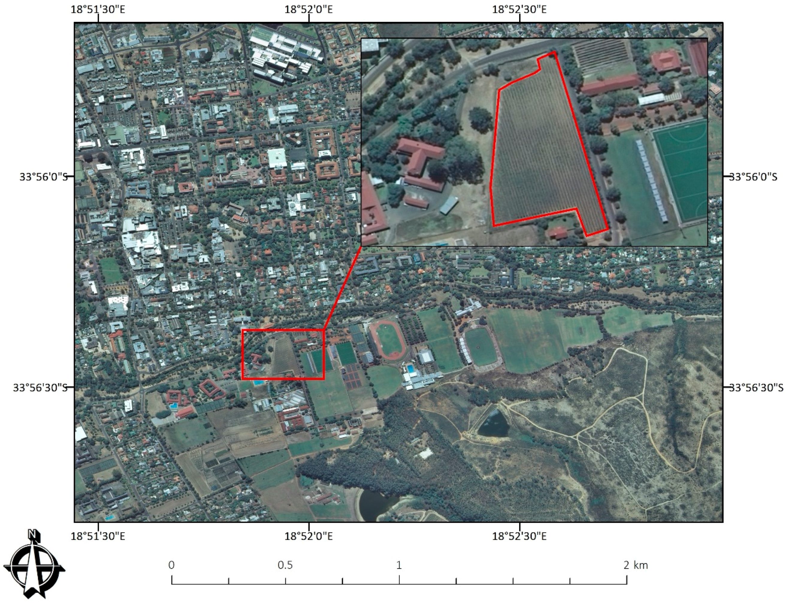
The study was conducted at the Welgevallen experimental farm in Stellenbosch (33°56′38.5′′S, 18°52′06.8′′E), situated in the Western Cape Province of South Africa (Figure 1). Stellenbosch has a Mediterranean climate characterised by dry summers and mild winters, with a mean annual temperature of 16.4 °C [38]. Stellenbosch receives low to moderate rainfall, mainly during the winter months (June, July, and August), with an annual average of 802 mm [38], making water scarcity a real threat to irrigated vineyards. Soil deposits in the region comprise rich potassium minerals that are favourable for vineyard growth [38]. The Welgevallen experimental farm comprises well-established grape cultivars, including Shiraz and Pinotage; Pinotage being a red cultivar unique to South Africa. Welgevallen is used by Stellenbosch University for research and training, and additionally produces high-quality grapes for commercial use.
2.2. Data Acquisition and Pre-Processing
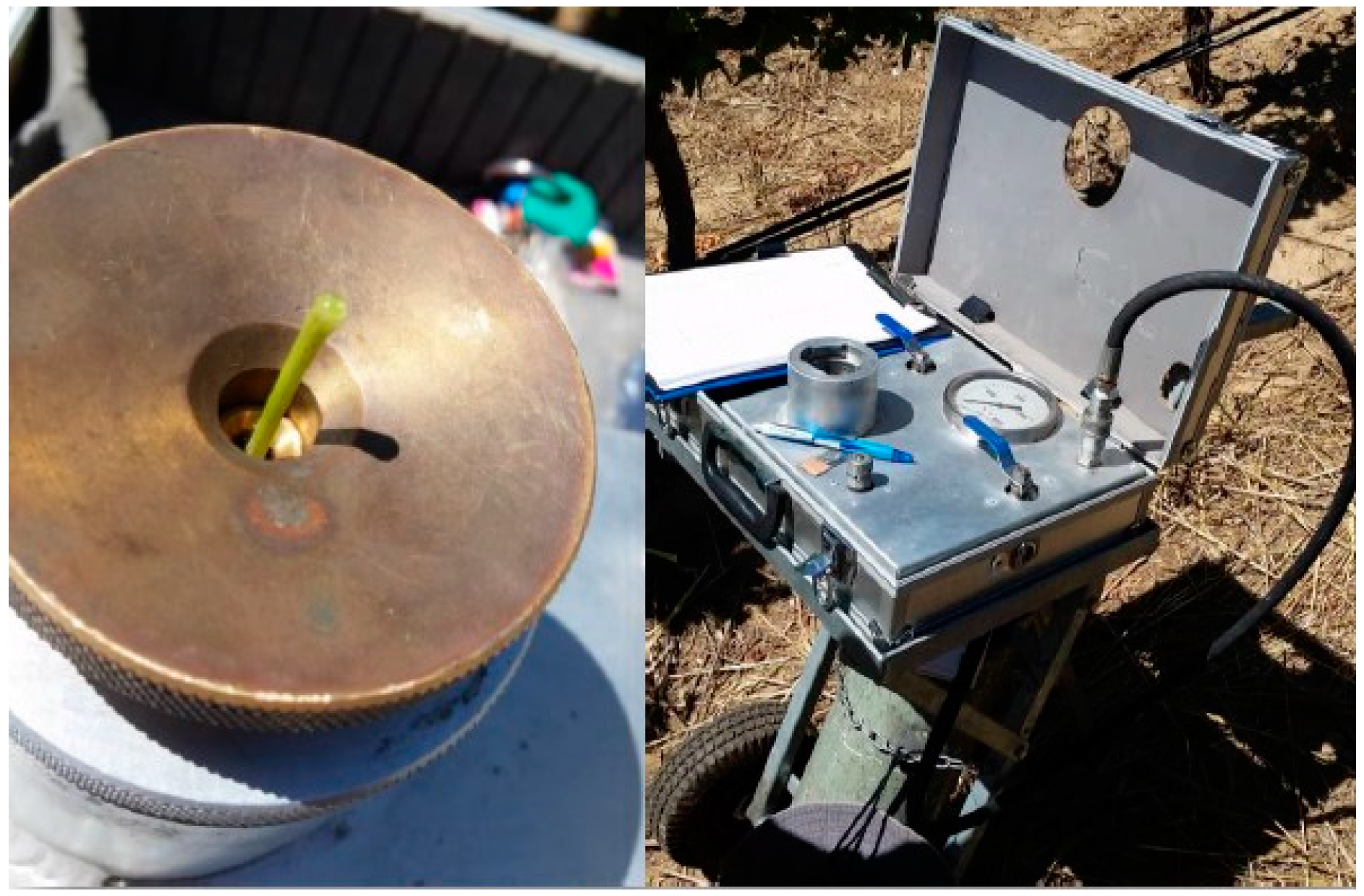
To confirm the water stress status of vines, in-field stem water potential (SWP) measurements were captured using a customised pressure chamber (Figure 2) as used by [39,40]. Based on the experiments by [39,41], vines with SWP values ranging from −1.0 MPa to −1.8 MPa were classified as water-stressed, whereas vines with SWP values ≥ −0.7 MPa were classified as non-stressed. Imaging spectrometer data was subsequently acquired for a water-stressed and non-stressed Shiraz vine. Images were captured between 10:00 and 12:00, on 24 February 2017, to ensure that the side of the vine canopy being captured was fully sunlit.
Images were captured using the SIMERA HX MkII hyperspectral sensor (SIMERA Technology Group, Somerset West South Africa). The sensor is a line scanner that captures 340 spectral wavebands across the VIS and NIR, i.e., 450–1000 nm, with a sensor bandwidth ranging from 0.9 nm to 5 nm. The sensor was mounted on a tripod (Figure 3A) to facilitate the collection of terrestrial imagery from a side-on view of the vine canopy. The sensor-tripod assembly was placed at a constant distance of one metre from the vine canopy to ensure that the full canopy of a single vine (approximately 1.4 m W × 1 m H) was captured per image (Figure 3B).
Due to sensor sensitivity and a deteriorating silicon chip, not all the wavebands could be utilised. Spectral subsets were, therefore, created per image. The spectral subsets consisted of 176 wavebands with a spectral range of 473–708 nm. Thereafter, raw image DN’s were converted to reflectance using the empirical line correction algorithm [42]. Empirical line correction uses known field (or reference) reflectance spectra and linear regression to equate digital number (DN) values to surface reflectance by estimating correction coefficients for each waveband [42]. Following [42], a white reference panel, positioned in the vine canopy prior to image capture, was used for image correction. Image pre-processing was performed in the Environment for Visualising Images (ENVI) version 5.3.1 software. Using a 2 × 2 pixel region of interest (ROI), a total of 60 leaf spectra were extracted from each image—30 samples per class (stressed and non-stressed)—and used as the input for classification.
2.3. Spectral Smoothing
In-field spectral measurements are often subjected to noise due to variable sun illumination [43]. Therefore, it is recommended that spectral smoothing be performed in order to produce a spectral signal that represents the original spectra without the interference of noise [44]. The Savitzky-Golay filter [45] is a common smoothing technique used in hyperspectral remote sensing [43,46,47]. Savitzky-Golay is based on least-squares approximation, which determines smoothing coefficients by applying a polynomial equation of a given degree and cluster size [45]. The filter is ideal for spectroscopic data as it minimises signal noise whilst preserving the originality and shape of the input spectra. A second order polynomial filter with a filter size of 15 was applied to the spectral samples prior to classification, following the recommendations of [47]. The Savitzky-Golay filter was applied using the ‘signal’ package [48] in the R statistical software environment [49]. Classification models were produced for both the unsmoothed and smoothed datasets.
2.4. Classification
2.4.1. Random Forest (RF)
The RF ensemble uses a bootstrap sample, i.e., 2/3 of the original dataset (referred to as the “in-bag” sample), to train decision trees. The remaining 1/3 of the data is used to compute an internal measure of accuracy (referred to as the “out-of-bag” or OOB error) [25]. To produce the forest of decision trees, two parameters need to be set: The number of unpruned trees to grow, known as ntree; and the number of predictor variables (i.e., wavebands) selected, known as mtry [25]. Mtry variables are tested at each node to specify the best split when growing trees. These randomly selected variables produce low correlated trees that prevent over-fitting. In a classification framework, the final classification results are determined by averaging the results of all the decision trees produced. For a detailed account of RF, see [25,50]. RF was implemented using the ‘randomForest’ package [51] in the R statistical software environment [49]. The default values for ntree (ntree = 500) and mtry (mtry = ) were used following [50,52].
2.4.2. Extreme Gradient Boosting (XGBoost)
XGBoost, like gradient boosting, is based on three essential elements; (i) a loss function that needs to be optimised; (ii) a multitude of weak decision trees that are used for classification; and (iii) an additive model that combines weak decision trees to produce a more accurate classification model [31]. XGBoost simultaneously optimises the loss function while constructing the additive model [30,31]. The loss function accounts for the errors in classification that were introduced by the weak decision trees [31]. For a detailed account of XGBoost, see [30]. XGBoost was implemented using the ‘xgboost’ package [53] in the R statistical software environment [49]. XGBoost requires the optimisation of several key parameters (Table 1). However, to facilitate a fair comparison of RF and XGBoost, the default values for all parameters were used to construct the XGBoost models, with nrounds set to 500. Furthermore, to ensure a more robust model and prevent overfitting, a 10-fold cross validation was performed for both RF and XGBoost.
2.5. Dimensionality Reduction
Both RF and XGBoost provide an internal measure of VI. RF provides two measures of VI, namely mean decrease Gini (MDG) and mean decrease accuracy (MDA) [25]. MDG quantifies VI by measuring the sum of all decreases in the Gini index, produced by a particular variable. MDA measures the changes in OOB error, which results from comparing the OOB error of the original dataset to that of a dataset created through random permutations of variable values. In this study, MDA was utilised to compute VI following the recommendations of [22,54,55]. The MDA VI for a waveband is defined by [56]:
where is the misclassification rate of tree t on the bootstrap sample not used to construct tree t, and is the error of predictor t on the permuted sample.
XGBoost ranks VI based on Gain [30]. Gain measures the degree of improved accuracy brought on by the addition of a given waveband. VI is calculated for each waveband, used for node splitting at a given tree, and then averaged across all trees to produce the final VI per waveband [30]. Similar to [23,24], the top 10% ( = 18) of the ranked waveband importance as determined by RF and XGBoost was used to create a subset of important wavebands. RF and XGBoost models were produced for both the original dataset and the subset of 18 wavebands.
2.6. Accuracy Assessment
To provide an independent estimate of model accuracy, an independent test set was used to evaluate all RF and XGBoost models. Therefore, a second dataset of spectral samples ( = 60) was collected for both stressed ( = 30) and non-stressed ( = 30) vines. Both algorithms were trained using the first dataset of 60 samples and tested using the second dataset. Overall classification accuracies were computed using a confusion matrix [57]. Additionally, Kappa analysis was used to evaluate model performance. The KHAT statistic [58] provides a measure of the difference between the actual and the chance agreement in the confusion matrix:
where describes the actual agreement and describes the chance agreement. Following [20,23,59], the McNemar’s test was employed to determine whether the differences in accuracies yielded by RF and XGBoost were statistically significant. Abdel-Rahman et al. [23] stated that the McNemar’s test can be expressed as the following chi-squared formula:
where denotes the number of samples misclassified by RF but correctly classified by XGBoost, and denotes the number of samples misclassified by XGBoost but correctly classified by RF. A value of greater than 3.84, at a 0.05 level of significance, indicates that the results of the two classifiers are significantly different [23,59].
3. Results
3.1. Spectral Smoothing Using the Savitzky-Golay Filter
Figure 4 shows the results of smoothing the spectral data using the Savitzky-Golay filter. It is evident that the Savitzky-Golay filter produced smoothed spectra without changing the shape of the original spectra. Additionally, the filter successfully preserved the original reflectance values, with the mean difference in reflectance values being less the than 0.3% with a standard deviation of 0.003 across all wavebands. All spectra ( = 120) were subsequently smoothed, and the smoothed spectra used as the input to classification.
3.2. Important Waveband Selection
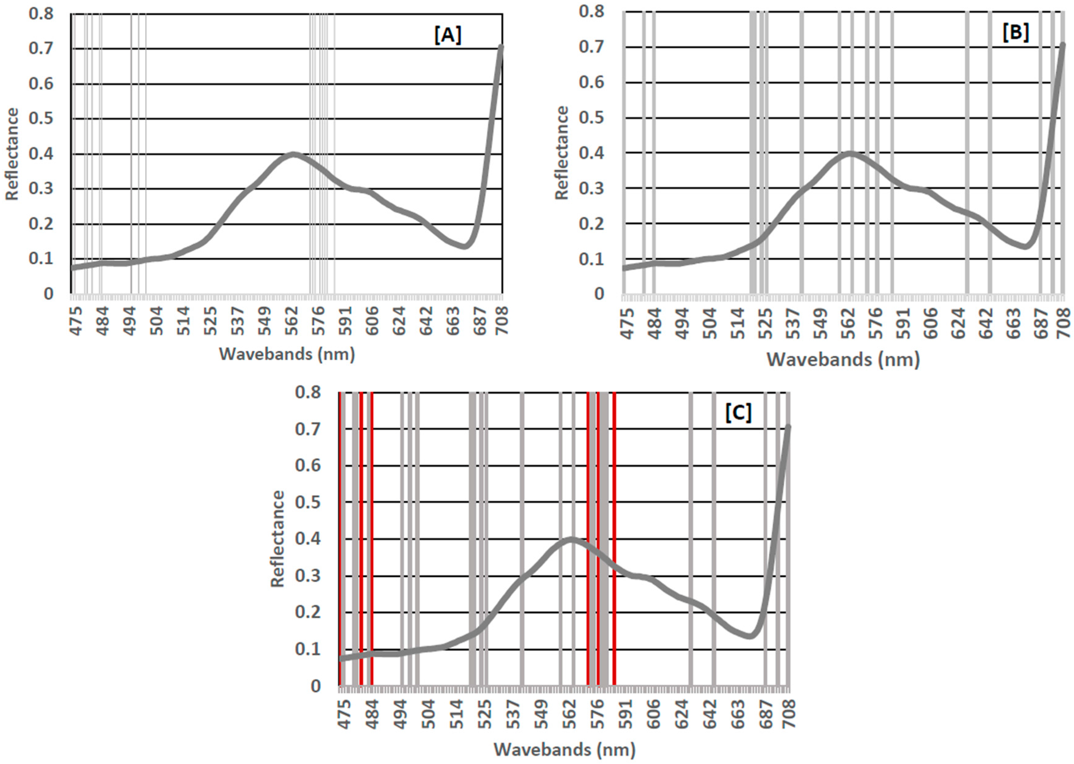
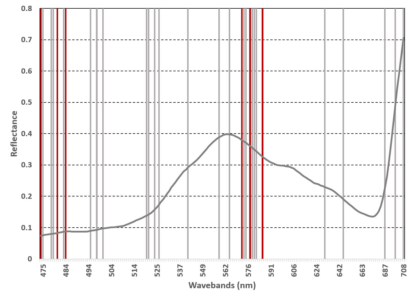
The top 10% ( = 18) of importance wavebands as determined by RF MDA and XGBoost gain are shown in Figure 5A,B, respectively. The results in Table 2 show that RF selected wavebands across blue and green (473.92–585.12 nm) regions of the EM spectrum. In comparison, XGBoost selected wavebands across the VIS (473.92–646.04 nm) and red-edge (686.69–708.32 nm) regions. It is evident from Figure 5 that the location of the wavebands selected by RF and XGBoost are significantly different. We attribute the difference in waveband location to the difference in VI measures used for RF and XGBoost. Nevertheless, as illustrated in Figure 5C, there were common wavebands selected by both RF and XGBoost. The overlapping wavebands ( = 6) were located across blue and green (473.92–585.12 nm) regions. Consequently, those wavebands may be the most important for discriminating between stressed and non-stressed Shiraz vines.
3.3. Classification Using Random Forest and Extreme Gradient Boosting
The classification results for RF and XGBoost are shown in Table 3 Training accuracies for all models were above 80.0%, with test accuracies ranging from 77.6% to 83.3% (with KHAT values ranging from 0.60 to 0.87). Overall, the results indicate that RF outperformed XGBoost, producing the highest accuracies for all the classification models.
Using all wavebands ( = 176), RF yielded a training accuracy of 90.0% (KHAT = 0.80) and a test accuracy of 83.3% (KHAT = 0.67). In comparison, XGBoost produced significantly lower accuracies, i.e., a training accuracy of 85.0% (KHAT = 0.7) and a test accuracy of 78.3% (KHAT = 0.57). These results indicate that the XGBoost ensemble resulted in reduced accuracies (approximately −5.0%) when using all wavebands to classify stressed and non-stressed Shiraz leaves.
Using the subset of important wavebands ( = 18) resulted in an overall improvement in classification accuracies for the RF and XGBoost. Training accuracy for RF increased by 3.3% to 93.3% (KHAT = 0.87). However, the test accuracy remained unchanged. Although XGBoost produced less accurate results, it did experience a greater increase in accuracy (5.0%), producing a training accuracy of 90.0% and a KHAT value of 0.8. The greater increase in accuracy may be attributed to the red-edge wavebands that were only present in the XGBoost subset. Moreover, the XGBoost subset also produced a slight increase (1.7%) in test accuracy (80.0%, KHAT = 0.6). We attribute the superior performance of the RF algorithm to its use of bootstrap sampling [25], which introduces model stability, and its robustness to noise [50].
Classification using the Savitzky-Golay smoothed spectra resulted in reduced accuracies overall. The decrease in accuracy ranged from 0.7–3.3% for all models. Furthermore, according to the McNemar’s test results, the difference in classifier performance was not statistically significant. For all the classification models, the chi-squared values were less than 3.84 with values ranging from 0.14 to 1.29.
4. Discussion
Ensemble classifiers, like RF and XGBoost, have been widely used to address the classification challenges inherent in high dimensional data [52]. The present study evaluated the use of terrestrial hyperspectral imaging to model vineyard water stress. More specifically, we tested the utility of two tree-based ensemble classifiers, namely RF and XGBoost, to model water stress in a Shiraz vineyard. The experimental results are discussed in further detail in the following sections.
4.1. Efficacy of the Savitzky-Golay Filter
The Savitzky-Golay filter has become a popular algorithm for smoothing spectroscopic data (for example, see [43,47,60]). In this study, the filter proved adept at smoothing the hyperspectral signature without significantly altering the originality of the input data. However, the results of this study showed that the filter negatively impacted the classification accuracy, producing reduced accuracies for RF (−1.6%) and XGBoost (−3.3%). The decrease in classification accuracy may be attributed to the specific parameter values used to implement the filter. The study only meant to test the functionality of the Savitzky-Golay filter. Therefore, the filter was implemented using the hyperparameter values as recommended by [47]. Consequently, the recommended values may not be optimal for the specific dataset used in this study.
Carvalho et al. [61] utilised the Savitzky-Golay filter to smooth magnetic flux leakage (MFL) signals. Similar to our study, the authors found that using the smoothed data with an ANN classifier, resulted in reduced classification accuracies. It is, therefore, evident that careful consideration has to be taken when applying the Savitzky-Golay filter.
4.2. Classification Using All Wavebands
Both tree-based ensemble classifiers tested in our study successfully demonstrated their efficiency for analysing hyperspectral data. However, our analysis found the RF bagging ensemble to outperform the boosting-based XGBoost ensemble when using all wavebands ( = 176).
Published comparisons between RF and boosting classifiers, similar to XGBoost, have reported mixed results. For example, Miao et al. [62] found that RF (93.5%) and AdaBoost (95.3%) produced similar overall accuracies when classifying ecological zones using multi-temporal and multi-sensor data. This is contrary to [62,63], which reported that RF outperformed boosting ensemble classifiers when classifying RADARSAT-1 imagery. Moreover, when directly comparing RF and XGBoost, within the context of spectroscopic classification, our findings contradict the results reported by [31]. Their study reported that XGBoost (96.0%) yielded significantly better results than RF (87.0%) when classifying supernovae. However, it should be noted that their study optimised RF and XGBoost parameters. More specifically, within viticulture, the results of our study compare favourably to those reported by [37]. The authors found that RF (87.8%) produced an improved accuracy compared to XGBoost (81.6%) when using hyperspectral data in combination with feature selection. A review by [50] concluded that RF generally achieves greater accuracies compared with boosting methods when used for the classification of high dimensional data such as hyperspectral imagery.
When comparing the utility of both algorithms, a key advantage shared between them is that RF and XGBoost effectively prevent overfitting [25,30]. However, given that RF grows trees independently (i.e., parallel to one another), whereas XGBoost grows trees sequentially, it is less complex and, therefore, less computationally intensive. Furthermore, RF requires the optimisation of only two parameters [25], whereas XGBoost has various parameters that could be optimised for a given dataset [30].
4.3. Classification Using Subset of Important Wavebands
Dimensionality reduction of hyperspectral data using machine learning has been extensively researched (for example see [20,22,23]). The results of our study indicate the VI ranking provided by RF and XGBoost can successfully be used to select a subset of wavebands for classification. This was evident from the increased accuracies obtained for both RF and XGBoost.
Our results compare favourably to those reported by [20,23], who demonstrated the feasibility of VI to reduce the high dimensionality of hyperspectral data and improve the classification accuracy. We, therefore, attribute the improved classification performance to the subset of most important wavebands. Although the subset of important wavebands did not result in massive accuracy gains (accuracy increase of RF ranged from 1.7% to 3.3% and from 0.7% to 3.3% for XGBoost), it did improve classification accuracy using only 10% of the original data. The majority of important wavebands, for RF ( = 9) and XGBoost ( = 10), were located in the green region of the EM spectrum (Table 2). The selected wavebands correspond to similar wavebands reported by [7,15]. The green region (i.e., between 500–600 nm) is highly sensitive to plant chlorophyll absorption [15]. Consequently, water stress in plants is closely related to lowered chlorophyll leaf concentrations [15], which can present a possible explanation for the selection of these wavebands.
Moreover, Shimada et al. [10] reported the use of the blue (490 nm) and red wavebands (620 nm) as indicators of plant water stress, and these wavebands correspond to similar wavebands present in the XGBoost subset (484.06 nm and 630.23 nm). In this study, only three red-edge wavebands (Table 2) were selected by XGBoost with none selected by RF. These results contradict those reported by [4], which found that wavebands in the red-edge region (695–730 nm) were ideal for early water stress detection in vineyards. However, given the overlapping wavebands that occur in the blue and green regions, and the results of our study, we can conclude that the red-edge wavebands may not be important for discriminating between stressed and non-stressed Shiraz vines. The results of this study subsequently demonstrate the feasibility of VIS wavebands to model water stress in a Shiraz vineyard.
Various aspects of the current research lend themselves to be operationalised within precision viticulture. For instance, the developed remote sensing-machine learning framework can be readily applied to model vegetative water stress. Furthermore, the identification of important wavebands can potentially lead to the construction of custom multispectral sensors that are less expensive and application specific.
5. Conclusions
This study presents a novel remote sensing-machine learning framework for modelling water stress in a Shiraz vineyard using terrestrial hyperspectral imaging. Based on the results of our study, we can draw the following conclusions:
- Both RF and XGBoost may be utilised to model water stress in a Shiraz vineyard.
- Wavebands in the VIS region of the EM spectrum may be used to model water stress in a Shiraz vineyard.
- It is imperative that future studies carefully consider the impact of applying the Savitzky-Golay filter for smoothing spectral data.
- The developed framework requires further investigation to evaluate its robustness and operational capabilities.
Given the results obtained in the present study, we recommend the employment of RF, rather than XGBoost, for the classification of hyperspectral data to discriminate stressed from non-stressed Shiraz vines.
Acknowledgments
Winetech funded the research. The authors sincerely thank the SIMERA Technology Group for providing the hyperspectral sensor.
Author Contributions
Kyle Loggenberg, Nitesh Poona, and Albert Strever conceptualised the research; Kyle Loggenberg conducted the field work, carried out the main analysis, and wrote the paper; Nitesh Poona and Berno Greyling assisted in data analysis and field work; Nitesh Poona contributed to the interpretation of the results. Nitesh Poona, Albert Strever, and Berno Greyling contributed to the editing of the manuscript.
Conflicts of Interest
The authors declare no conflict of interest.
References
- Costa, J.M.; Vaz, M.; Escalona, J.; Egipto, R.; Lopes, C.; Medrano, H.; Chaves, M.M. Modern viticulture in southern Europe: Vulnerabilities and strategies for adaptation to water scarcity. Agric. Water Manag. 2016, 164, 5–18. [Google Scholar] [CrossRef]
- Zarco-Tejada, P.J.; González-Dugo, V.; Berni, J.A.J. Fluorescence, temperature and narrow-band indices acquired from a UAV platform for water stress detection using a micro-hyperspectral imager and a thermal camera. Remote Sens. Environ. 2012, 117, 322–337. [Google Scholar] [CrossRef]
- Kim, Y.; Glenn, D.M.; Park, J.; Ngugi, H.K.; Lehman, B.L. Hyperspectral image analysis for water stress detection of apple trees. Comput. Electron. Agric. 2011, 77, 155–160. [Google Scholar] [CrossRef]
- Maimaitiyiming, M.; Ghulam, A.; Bozzolo, A.; Wilkins, J.L.; Kwasniewski, M.T. Early Detection of Plant Physiological Responses to Different Levels of Water Stress Using Reflectance Spectroscopy. Remote Sens. 2017, 9, 745. [Google Scholar] [CrossRef]
- Bota, J.; Tomás, M.; Flexas, J.; Medrano, H.; Escalona, J.M. Differences among grapevine cultivars in their stomatal behavior and water use efficiency under progressive water stress. Agric. Water Manag. 2016, 164, 91–99. [Google Scholar] [CrossRef]
- Chirouze, J.; Boulet, G.; Jarlan, L.; Fieuzal, R.; Rodriguez, J.C.; Ezzahar, J.; Er-Raki, S.; Bigeard, G.; Merlin, O.; Garatuza-Payan, J.; et al. Intercomparison of four remote-sensing-based energy balance methods to retrieve surface evapotranspiration and water stress of irrigated fields in semi-arid climate. Hydrol. Earth Syst. Sci. 2014, 18, 1165–1188. [Google Scholar] [CrossRef] [Green Version]
- Zarco-Tejada, P.J.; González-Dugo, V.; Williams, L.E.; Suárez, L.; Berni, J.A.J.; Goldhamer, D.; Fereres, E. A PRI-based water stress index combining structural and chlorophyll effects: Assessment using diurnal narrow-band airborne imagery and the CWSI thermal index. Remote Sens. Environ. 2013, 138, 38–50. [Google Scholar] [CrossRef]
- González-Fernández, A.B.; Rodríguez-Pérez, J.R.; Marcelo, V.; Valenciano, J.B. Using field spectrometry and a plant probe accessory to determine leaf water content in commercial vineyards. Agric. Water Manag. 2015, 156, 43–50. [Google Scholar] [CrossRef]
- Baluja, J.; Diago, M.P.; Balda, P.; Zorer, R.; Meggio, F.; Morales, F.; Tardaguila, J. Assessment of vineyard water status variability by thermal and multispectral imagery using an unmanned aerial vehicle (UAV). Irrig. Sci. 2012, 30, 511–522. [Google Scholar] [CrossRef]
- Shimada, S.; Funatsuka, E.; Ooda, M.; Takyu, M.; Fujikawa, T.; Toyoda, H. Developing the Monitoring Method for Plant Water Stress Using Spectral Reflectance Measurement. J. Arid Land Stud. 2012, 22, 251–254. [Google Scholar]
- Govender, M.; Dye, P.; Witokwski, E.; Ahmed, F. Review of commonly used remote sensing and ground based technologies to measure plant water stress. Water SA 2009, 35, 741–752. [Google Scholar] [CrossRef]
- De Bei, R.; Cozzolino, D.; Sullivan, W.; Cynkar, W.; Fuentes, S.; Dambergs, R.; Pech, J.; Tyerman, S.D. Non-destructive measurement of grapevine water potential using near infrared spectroscopy. Aust. J. Grape Wine Res. 2011, 17, 62–71. [Google Scholar] [CrossRef]
- Diago, M.P.; Bellincontro, A.; Scheidweiler, M.; Tardaguila, J.; Tittmann, S.; Stoll, M. Future opportunities of proximal near infrared spectroscopy approaches to determine the variability of vineyard water status. Aust. J. Grape Wine Res. 2017, 23, 409–414. [Google Scholar] [CrossRef]
- Beghi, R.; Giovenzana, V.; Guidetti, R. Better water use efficiency in vineyard by using visible and near infrared spectroscopy for grapevine water status monitoring. Chem. Eng. Trans. 2017, 58, 691–696. [Google Scholar] [CrossRef]
- Pôças, I.; Rodrigues, A.; Gonçalves, S.; Costa, P.M.; Gonçalves, I.; Pereira, L.S.; Cunha, M. Predicting grapevine water status based on hyperspectral reflectance vegetation indices. Remote Sens. 2015, 7, 16460–16479. [Google Scholar] [CrossRef]
- Carreiro Soares, S.F.; Medeiros, E.P.; Pasquini, C.; de Lelis Morello, C.; Harrop Galvão, R.K.; Ugulino Araújo, M.C. Classification of individual cotton seeds with respect to variety using near-infrared hyperspectral imaging. Anal. Methods 2016, 8, 8498–8505. [Google Scholar] [CrossRef]
- Mulla, D.J. Twenty five years of remote sensing in precision agriculture: Key advances and remaining knowledge gaps. Biosyst. Eng. 2013, 114, 358–371. [Google Scholar] [CrossRef]
- Poona, N.K.; Van Niekerk, A.; Nadel, R.L.; Ismail, R. Random Forest (RF) Wrappers for Waveband Selection and Classification of Hyperspectral Data. Appl. Spectrosc. 2016, 70, 322–333. [Google Scholar] [CrossRef] [PubMed]
- Hughes, G.F. On the mean accuracy of statistical pattern recognizers. IEEE Trans. Inf. Theory 1968, 14, 55–63. [Google Scholar] [CrossRef]
- Pedergnana, M.; Marpu, P.R.; Mura, M.D. A Novel Technique for Optimal Feature Selection in Attribute Profiles Based on Genetic Algorithms. IEEE Trans. Geosci. Remote Sens. 2013, 51, 3514–3528. [Google Scholar] [CrossRef]
- Tong, Q.; Xue, Y.; Zhang, L. Progress in hyperspectral remote sensing science and technology in China over the past three decades. IEEE J. Sel. Top. Appl. Earth Obs. Remote Sens. 2014, 7, 70–91. [Google Scholar] [CrossRef]
- Poona, N.K.; Ismail, R. Using Boruta-selected spectroscopic wavebands for the asymptomatic detection of fusarium circinatum stress. IEEE J. Sel. Top. Appl. Earth Obs. Remote Sens. 2014, 7, 3764–3772. [Google Scholar] [CrossRef]
- Abdel-Rahman, E.M.; Mutanga, O.; Adam, E.; Ismail, R. Detecting Sirex noctilio grey-attacked and lightning-struck pine trees using airborne hyperspectral data, random forest and support vector machines classifiers. ISPRS J. Photogramm. Remote Sens. 2014, 88, 48–59. [Google Scholar] [CrossRef]
- Corcoran, J.M.; Knight, J.F.; Gallant, A.L. Influence of multi-source and multi-temporal remotely sensed and ancillary data on the accuracy of random forest classification of wetlands in northern Minnesota. Remote Sens. 2013, 5, 3212–3238. [Google Scholar] [CrossRef]
- Breiman, L. Random forests. Mach. Learn. 2001, 45, 5–32. [Google Scholar] [CrossRef]
- Abdel-Rahman, E.M.; Makori, D.M.; Landmann, T.; Piiroinen, R.; Gasim, S.; Pellikka, P.; Raina, S.K. The utility of AISA eagle hyperspectral data and random forest classifier for flower mapping. Remote Sens. 2015, 7, 13298–13318. [Google Scholar] [CrossRef]
- Adam, E.; Deng, H.; Odindi, J.; Abdel-Rahman, E.M.; Mutanga, O. Detecting the Early Stage of Phaeosphaeria Leaf Spot Infestations in Maize Crop Using In Situ Hyperspectral Data and Guided Regularized Random Forest Algorithm. J. Spectrosc. 2017, 2017. [Google Scholar] [CrossRef]
- Sandika, B.; Avil, S.; Sanat, S.; Srinivasu, P. Random forest based classification of diseases in grapes from images captured in uncontrolled environments. In Proceedings of the IEEE 13th International Conference, Signal Processing Proceedings, Chengdu, China, 6–10 November 2016; pp. 1775–1780. [Google Scholar]
- Knauer, U.; Matros, A.; Petrovic, T.; Zanker, T.; Scott, E.S.; Seiffert, U. Improved classification accuracy of powdery mildew infection levels of wine grapes by spatial-spectral analysis of hyperspectral images. Plant Methods 2017, 13. [Google Scholar] [CrossRef] [PubMed]
- Chen, T.; Guestrin, C. XGBoost: A Scalable Tree Boosting System. In Proceedings of the 22nd ACM Sigkdd International Conference on Knowledge Discovery and Data Mining, San Francisco, CA, USA, 13–17 August 2016; pp. 785–794. [Google Scholar]
- Möller, A.; Ruhlmann-Kleider, V.; Leloup, C.; Neveu, J.; Palanque-Delabrouille, N.; Rich, J.; Carlberg, R.; Lidman, C.; Pritchet, C. Photometric classification of type Ia supernovae in the SuperNova Legacy Survey with supervised learning. J. Cosmol. Astropart. Phys. 2016, 12. [Google Scholar] [CrossRef]
- Torlay, L.; Perrone-Bertolotti, M.; Thomas, E.; Baciu, M. Machine learning–XGBoost analysis of language networks to classify patients with epilepsy. Brain Inform. 2017, 4, 159–169. [Google Scholar] [CrossRef] [PubMed]
- Fitriah, N.; Wijaya, S.K.; Fanany, M.I.; Badri, C.; Rezal, M. EEG channels reduction using PCA to increase XGBoost’s accuracy for stroke detection. AIP Conf. Proc. 2017, 1862, 30128. [Google Scholar] [CrossRef]
- Friedman, J. Greedy function approximation: A gradient boosting machine. Ann. Stat. 2001, 29, 1189–1232. [Google Scholar] [CrossRef]
- Ren, X.; Guo, H.; Li, S.; Wang, S. A Novel Image Classification Method with CNN-XGBoost Model. In International Workshop on Digital Watermarking; Springer: Cham, Switzerland, 2017; pp. 378–390. [Google Scholar]
- Friedman, J.H. Stochastic gradient boosting. Comput. Stat. Data Anal. 2002, 38, 367–378. [Google Scholar] [CrossRef]
- Mohite, J.; Karale, Y.; Pappula, S.; Shabeer, T.P.; Sawant, S.D.; Hingmire, S. Detection of pesticide (Cyantraniliprole) residue on grapes using hyperspectral sensing. In Sensing for Agriculture and Food Quality and Safety IX, Proceedings of the SPIE Commercial+ Scientific Sensing and Imaging Conference, Anaheim, CA, USA, 1 May 2017; Kim, M.S., Chao, K.L., Chin, B.A., Cho, B.K., Eds.; International Society for Optics and Photonics: Bellingham, WA, USA, 2017. [Google Scholar]
- Conradie, W.J.; Carey, V.A.; Bonnardot, V.; Saayman, D.; Van Schoor, L.H. Effect of Different Environmental Factors on the Performance of Sauvignon blanc Grapevines in the Stellenbosch/Durbanville Districts of South Africa I. Geology, Soil, Climate, Phenology and Grape Composition. S. Afr. J. Enol. Vitic. 2002, 23, 78–91. [Google Scholar]
- Deloire, A.; Heyms, D. The leaf water potentials: Principles, method and thresholds. Wynboer 2011, 265, 119–121. [Google Scholar]
- Choné, X.; Van Leeuwen, C.; Dubourdieu, D.; Gaudillère, J.P. Stem water potential is a sensitive indicator of grapevine water status. Ann. Bot. 2001, 87, 477–483. [Google Scholar] [CrossRef]
- Myburgh, P.; Cornelissen, M.; Southey, T. Interpretation of Stem Water Potential Measurements. WineLand. 2016, pp. 78–80. Available online: http://www.wineland.co.za/interpretation-of-stem-water-potential-measurements/ (accessed on 26 January 2018).
- Aasen, H.; Burkart, A.; Bolten, A.; Bareth, G. Generating 3D hyperspectral information with lightweight UAV snapshot cameras for vegetation monitoring: From camera calibration to quality assurance. ISPRS J. Photogramm. Remote Sens. 2015, 108, 245–259. [Google Scholar] [CrossRef]
- Schmidt, K.S.; Skidmore, A.K. Smoothing vegetation spectra with wavelets. Int. J. Remote Sens. 2004, 25, 1167–1184. [Google Scholar] [CrossRef]
- Člupek, M.; Matějka, P.; Volka, K. Noise reduction in Raman spectra: Finite impulse response filtration versus Savitzky–Golay smoothing. J. Raman Spectrosc. 2007, 38, 1174–1179. [Google Scholar] [CrossRef]
- Savitzky, A.; Golay, M.J. Smoothing and differentiation of data by simplified least squares procedures. Anal. Chem. 1964, 36, 1627–1639. [Google Scholar] [CrossRef]
- Liu, L.; Ji, M.; Dong, Y.; Zhang, R.; Buchroithner, M. Quantitative Retrieval of Organic Soil Properties from Visible Near-Infrared Shortwave Infrared Feature Extraction. Remote Sens. 2016, 8, 1035. [Google Scholar] [CrossRef]
- Prasad, K.A.; Gnanappazham, L.; Selvam, V.; Ramasubramanian, R.; Kar, C.S. Developing a spectral library of mangrove species of Indian east coast using field spectroscopy. Geocarto Int. 2015, 30, 580–599. [Google Scholar] [CrossRef]
- Ligges, U.; Short, T.; Kienzle, P.; Schnackenberg, S.; Billinghurst, S.; Borchers, H.-W.; Carezia, A.; Dupuis, P.; Eaton, J.W.; Farhi, E.; et al. Signal: Signal Processing. 2015. Available online: http://docplayer.net/24709837-Package-signal-july-30-2015.html (accessed on 26 January 2018).
- R Development Core Team, R. R: A Language and Environment for Statistical Computing; R Foundation for Statistical Computing: Vienna, Austria, 2017. [Google Scholar]
- Belgiu, M.; Drăguţ, L. Random forest in remote sensing: A review of applications and future directions. ISPRS J. Photogramm. Remote Sens. 2016, 114, 24–31. [Google Scholar] [CrossRef]
- Liaw, A.; Wiener, M. Classification and Regression by randomForest. R News 2002, 2, 18–22. [Google Scholar] [CrossRef]
- Poona, N.; van Niekerk, A.; Ismail, R. Investigating the utility of oblique tree-based ensembles for the classification of hyperspectral data. Sensors 2016, 16. [Google Scholar] [CrossRef] [PubMed]
- Chen, T.; He, T.; Benesty, M.; Khotilovich, V.; Tang, Y. Xgboost: Extreme Gradient Boosting. 2017. Available online: https://cran.r-project.org/package=xgboost (accessed on 26 January 2018).
- Immitzer, M.; Atzberger, C.; Koukal, T. Tree species classification with Random forest using very high spatial resolution 8-band WorldView-2 satellite data. Remote Sens. 2012, 4, 2661–2693. [Google Scholar] [CrossRef]
- Belgiu, M.; Tomljenovic, I.; Lampoltshammer, T.J.; Blaschke, T.; Höfle, B. Ontology-based classification of building types detected from airborne laser scanning data. Remote Sens. 2014, 6, 1347–1366. [Google Scholar] [CrossRef]
- Genuer, R.; Poggi, J.-M.; Tuleau-Malot, C. Variable selection using random forests. Pattern Recognit. Lett. 2010, 31, 2225–2236. [Google Scholar] [CrossRef]
- Kohavi, R.; Provost, F. Glossary of terms. Mach. Learn. 1998, 30, 271–274. [Google Scholar]
- Congalton, R.G.; Green, K. Assessing the Accuracy of Remotely Sensed Data: Principles and Practices, 2nd ed.; CRC Press: Boco Raton, FL, USA, 2008. [Google Scholar]
- Foody, G.M. Thematic map comparison: Evaluating the statistical significance of differences in classification accuracy. Photogramm. Eng. Remote Sens. 2004, 70, 627–633. [Google Scholar] [CrossRef]
- Gutiérrez, S.; Tardaguila, J.; Fernández-Novales, J.; Diago, M.P. Data mining and NIR spectroscopy in viticulture: Applications for plant phenotyping under field conditions. Sensors 2016, 16, 236. [Google Scholar] [CrossRef] [PubMed]
- Carvalho, A.A.; Rebello, J.M.A.; Sagrilo, L.V.S.; Camerini, C.S.; Miranda, I.V.J. MFL signals and artificial neural networks applied to detection and classification of pipe weld defects. NDT E Int. 2006, 39, 661–667. [Google Scholar] [CrossRef]
- Miao, X.; Heaton, J.S.; Zheng, S.; Charlet, D.A.; Liu, H. Applying tree-based ensemble algorithms to the classification of ecological zones using multi-temporal multi-source remote-sensing data. Int. J. Remote Sens. 2012, 33, 1823–1849. [Google Scholar] [CrossRef]
- Xu, L.; Li, J.; Brenning, A. A comparative study of different classification techniques for marine oil spill identification using RADARSAT-1 imagery. Remote Sens. Environ. 2014, 141, 14–23. [Google Scholar] [CrossRef]
Figure 1.
Location of the Welgevallen Shiraz vineyard plot used in this study. Background image provided by National Geo-Spatial Information (NGI) (2012).
Figure 1.
Location of the Welgevallen Shiraz vineyard plot used in this study. Background image provided by National Geo-Spatial Information (NGI) (2012).

Figure 2.
Customised pressure chamber used to measure Stem Water Potential.

Figure 3.
The hyperspectral sensor tripod assembly (A); and in-field setup when collecting terrestrial imagery of the vine canopy (B).
Figure 3.
The hyperspectral sensor tripod assembly (A); and in-field setup when collecting terrestrial imagery of the vine canopy (B).
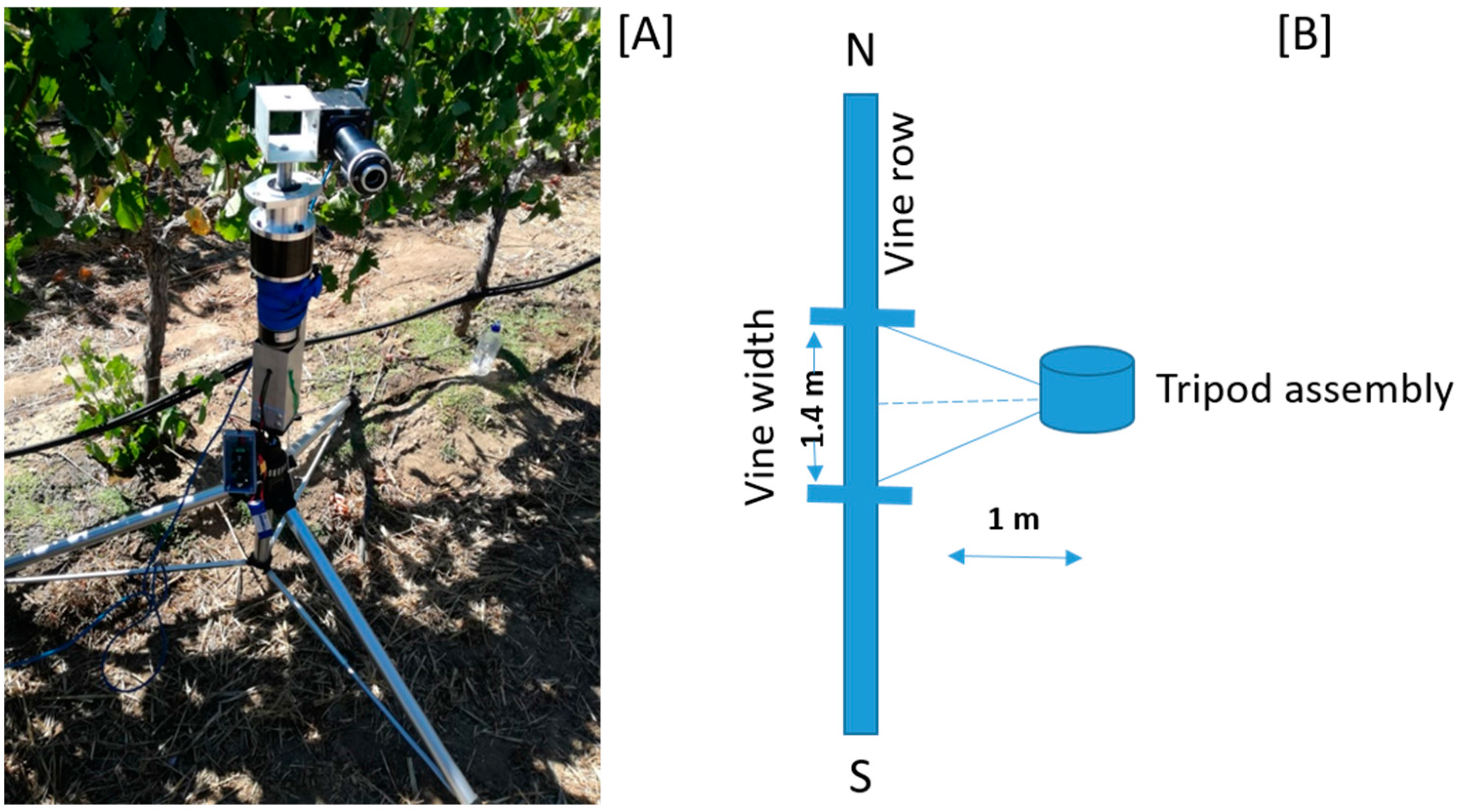
Figure 4.
Spectra comparison before (red) and after (black) applying Savitzky-Golay filter.
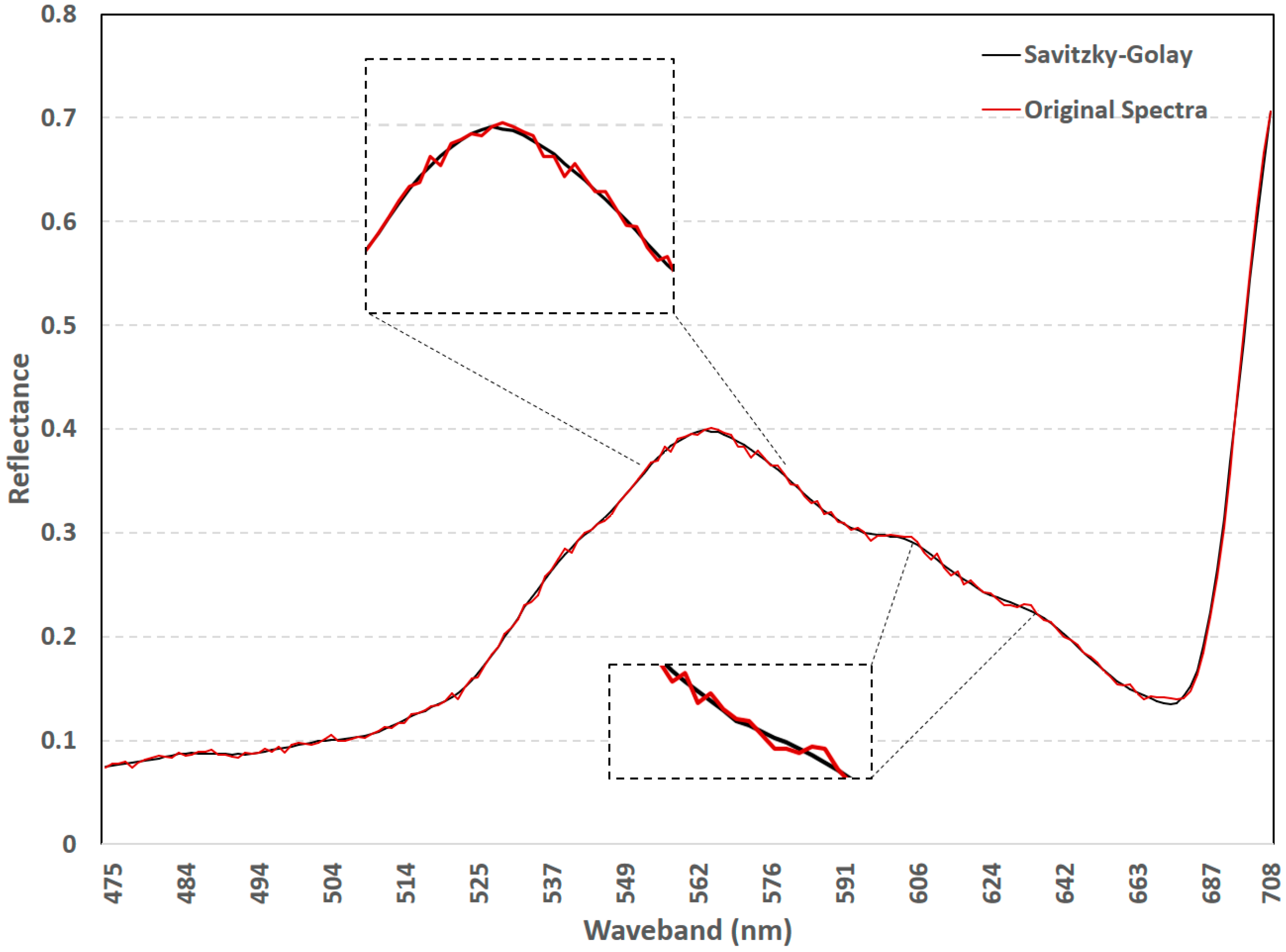
Figure 5.
The importance wavebands as determined by RF (A); XGBoost (B); and overlapping (C). The grey bars represent the important wavebands selected by RF and XGBoost, respectively. The red bars indicate the overlapping wavebands. The mean spectral signature of a sample is shown as a reference.
Figure 5.
The importance wavebands as determined by RF (A); XGBoost (B); and overlapping (C). The grey bars represent the important wavebands selected by RF and XGBoost, respectively. The red bars indicate the overlapping wavebands. The mean spectral signature of a sample is shown as a reference.

Table 1.
Key parameters used for XGBoost classification.
| Parameter | Description | Default Value |
|---|---|---|
| max_depth | controls the maximum depth of each tree (used to control over-fitting) | 6 |
| subsample | specifies the fraction of observations to be randomly sampled at each tree (adds randomness) | 1 |
| eta | the learning rate | 0.3 |
| nrounds | the number of trees to be produced (similar to ntree) | 100–1000 |
| gamma | controls the minimum loss reduction required to make a node split (used to control over-fitting) | 0 |
| min_child_weight | Specifies the minimum sum of instance weight of all the observations required in a child (used to control over-fitting) | 1 |
| colsample_bytree | Specifies the number of features to consider when searching for the best node split (adds randomness) | 1 |
Table 2.
Location of the RF and XGBoost selected important wavebands in the EM spectrum.
| VIS (473 nm–680 nm) | Red-Edge (680 nm–708 nm) | |||
|---|---|---|---|---|
| RF | 12 | 474.74, 478.09, 478.94, 483.2, 494.64, 497.36, 500.11, 573.31, 574.59, 578.48, 579.79, 581.11 | 0 | - |
| XGBoost | 9 | 520.31, 521.32, 524.36, 526.42, 541.34, 558.52, 564.56,630.23, 646.04 | 3 | 686.69, 698.39, 708.32 |
| Overlap | 6 | 473.92, 480.63, 484.06 572.04, 577.17, 585.12 | 0 | - |
Table 3.
Classification accuracies of both the RF and XGBoost models constructed using all the wavebands and the subset of important wavebands.
Table 3.
Classification accuracies of both the RF and XGBoost models constructed using all the wavebands and the subset of important wavebands.
| All Wavebands ( = 176) | Important Wavebands ( = 18) | ||||||||
|---|---|---|---|---|---|---|---|---|---|
| Train | Test | Train | Test | ||||||
| Accuracy (%) | Kappa | Accuracy (%) | Kappa | Accuracy (%) | Kappa | Accuracy (%) | Kappa | ||
| XGBoost | Unsmoothed | 85.0 | 0.70 | 78.3 | 0.57 | 90.0 | 0.80 | 80.0 | 0.60 |
| Smoothed | 83.3 | 0.67 | 77.6 | 0.53 | 86.7 | 0.73 | 78.3 | 0.57 | |
| RF | Unsmoothed | 90.0 | 0.80 | 83.3 | 0.67 | 93.3 | 0.87 | 83.3 | 0.67 |
| Smoothed | 90.0 | 0.80 | 81.7 | 0.63 | 91.7 | 0.83 | 81.7 | 0.63 | |
© 2018 by the authors. Licensee MDPI, Basel, Switzerland. This article is an open access article distributed under the terms and conditions of the Creative Commons Attribution (CC BY) license (http://creativecommons.org/licenses/by/4.0/).
Share and Cite
MDPI and ACS Style
Loggenberg, K.; Strever, A.; Greyling, B.; Poona, N. Modelling Water Stress in a Shiraz Vineyard Using Hyperspectral Imaging and Machine Learning. Remote Sens. 2018, 10, 202. https://doi.org/10.3390/rs10020202
AMA Style
Loggenberg K, Strever A, Greyling B, Poona N. Modelling Water Stress in a Shiraz Vineyard Using Hyperspectral Imaging and Machine Learning. Remote Sensing. 2018; 10(2):202. https://doi.org/10.3390/rs10020202
Chicago/Turabian StyleLoggenberg, Kyle, Albert Strever, Berno Greyling, and Nitesh Poona. 2018. "Modelling Water Stress in a Shiraz Vineyard Using Hyperspectral Imaging and Machine Learning" Remote Sensing 10, no. 2: 202. https://doi.org/10.3390/rs10020202
Note that from the first issue of 2016, this journal uses article numbers instead of page numbers. See further details here.