Detecting Neolithic Burial Mounds from LiDAR-Derived Elevation Data Using a Multi-Scale Approach and Machine Learning Techniques

Abstract
:
1. Introduction
1.1. Archaeological Context
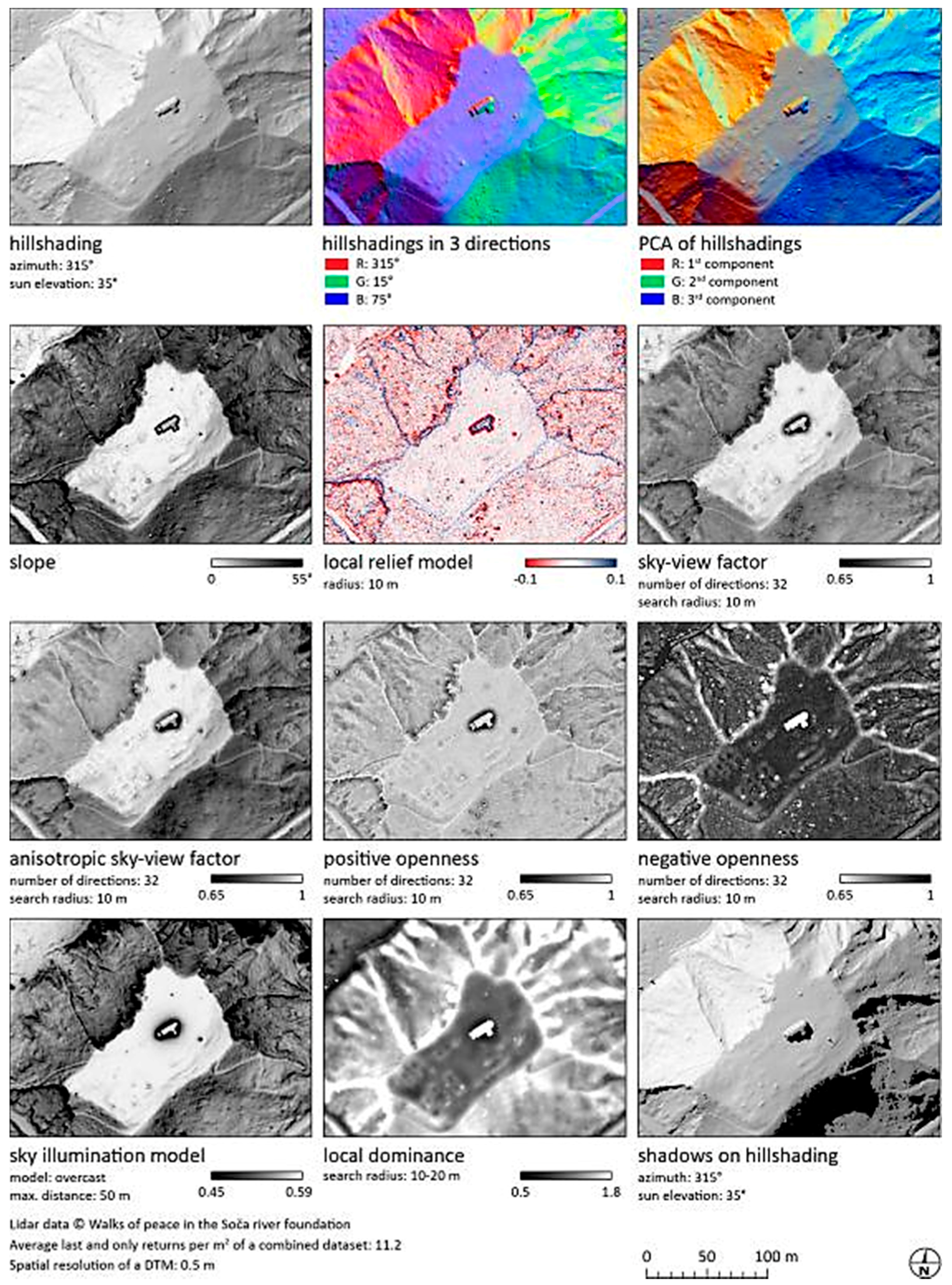
1.2. Terrain Visualisation Techniques
1.3. Machine Learning and Classification Techniques
2. Materials and Methods
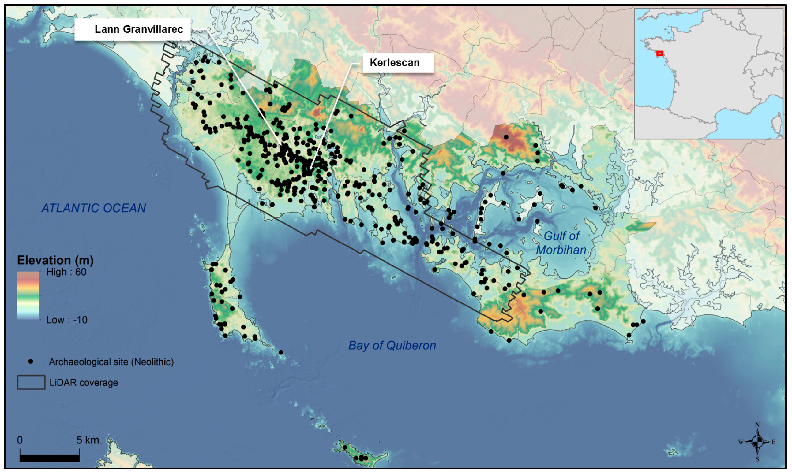
2.1. Study Area
2.2. LiDAR Data
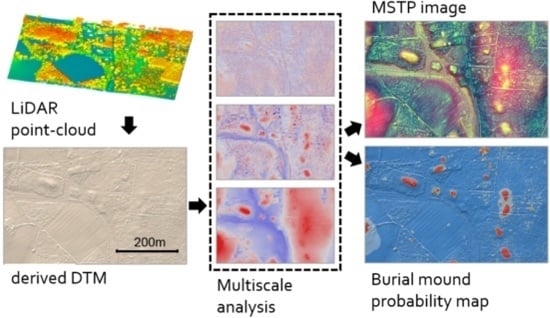
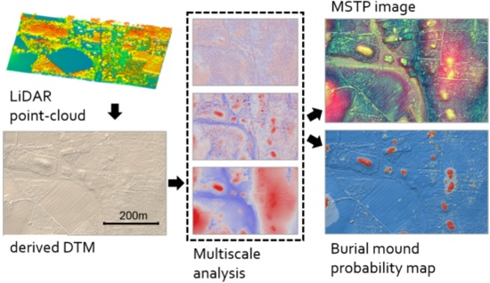
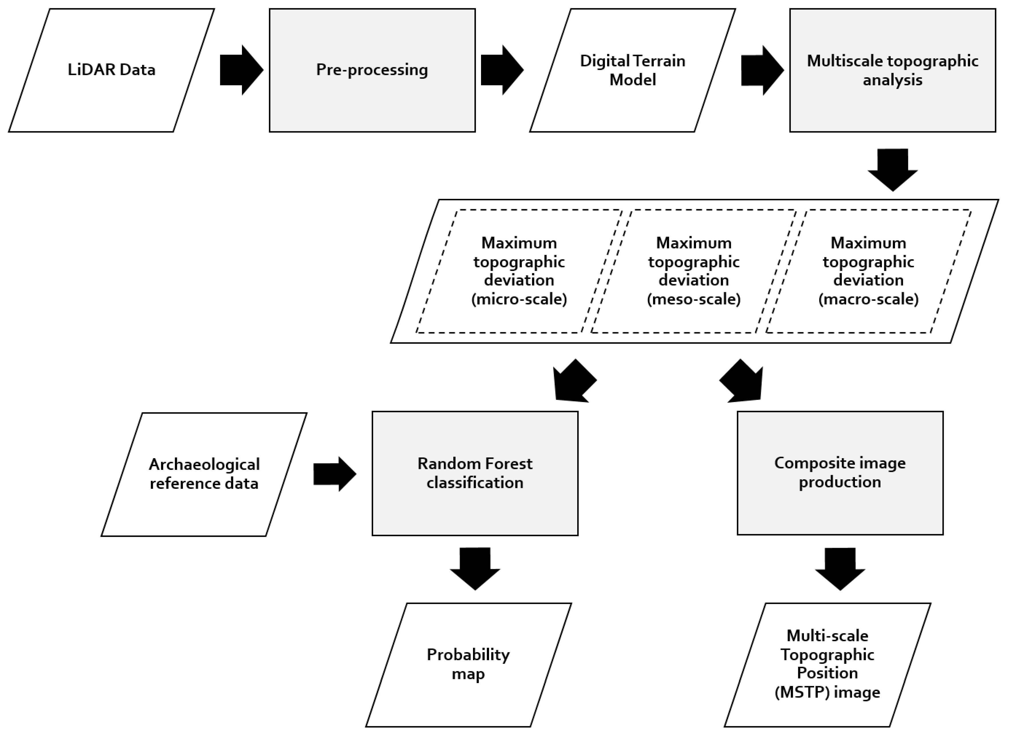
2.3. The Method
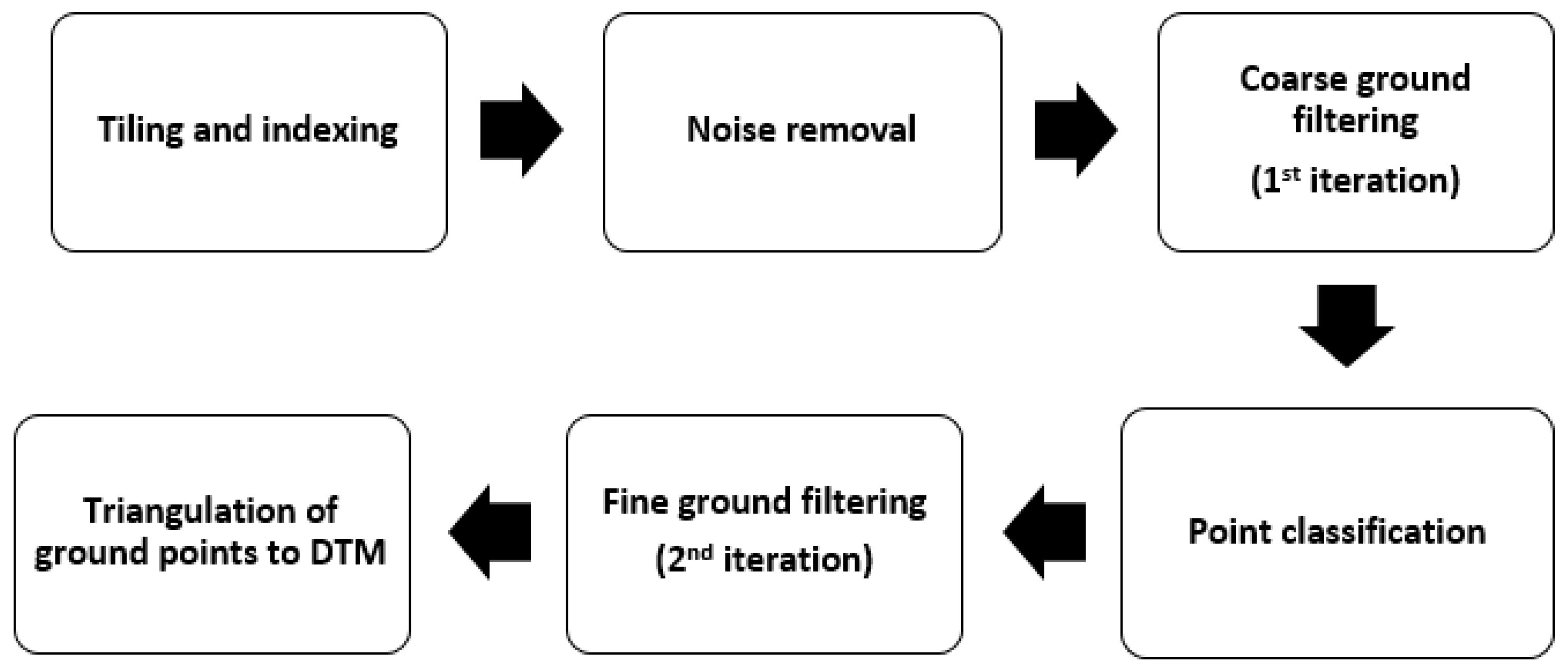
2.3.1. Pre-Processing of LiDAR Data
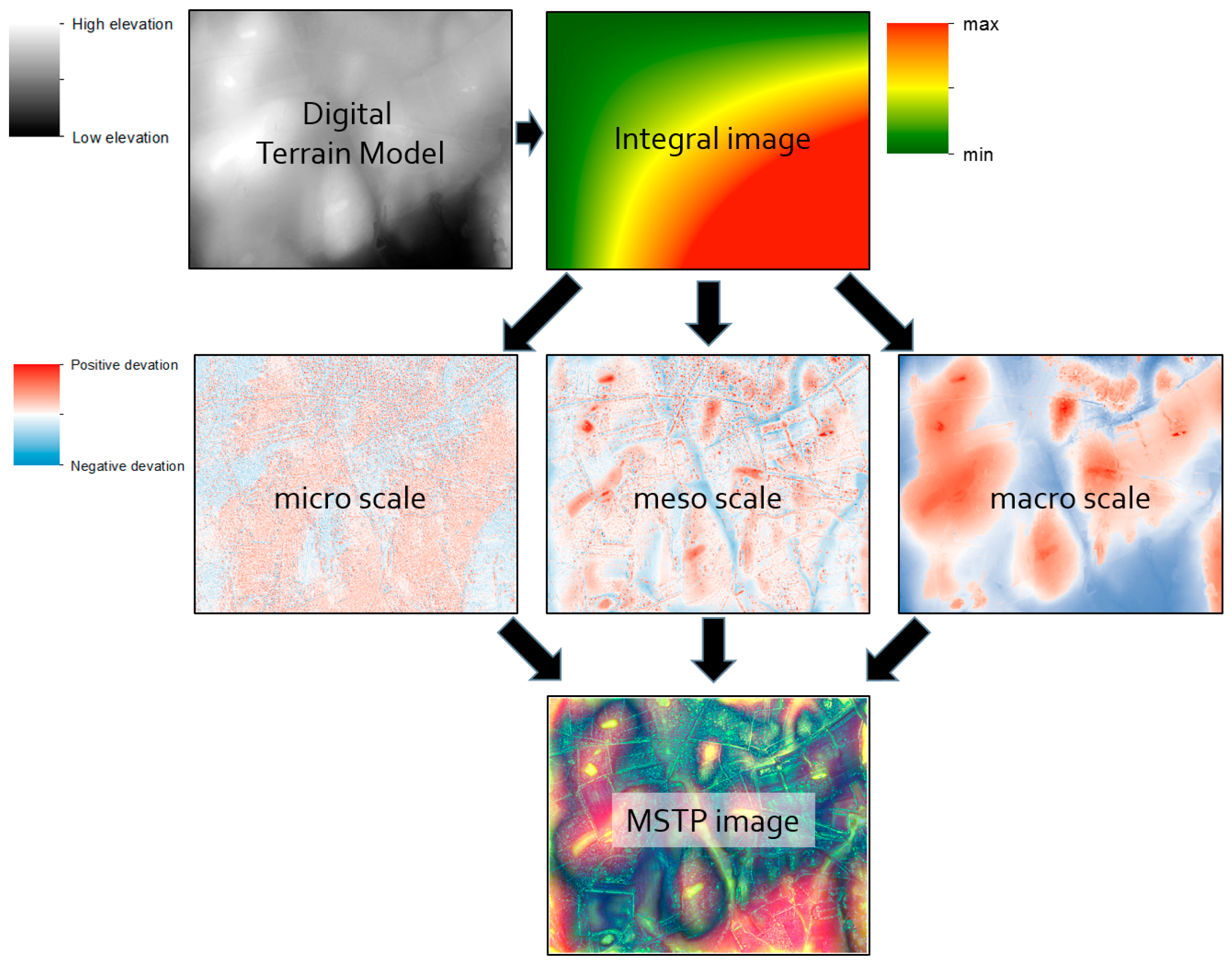
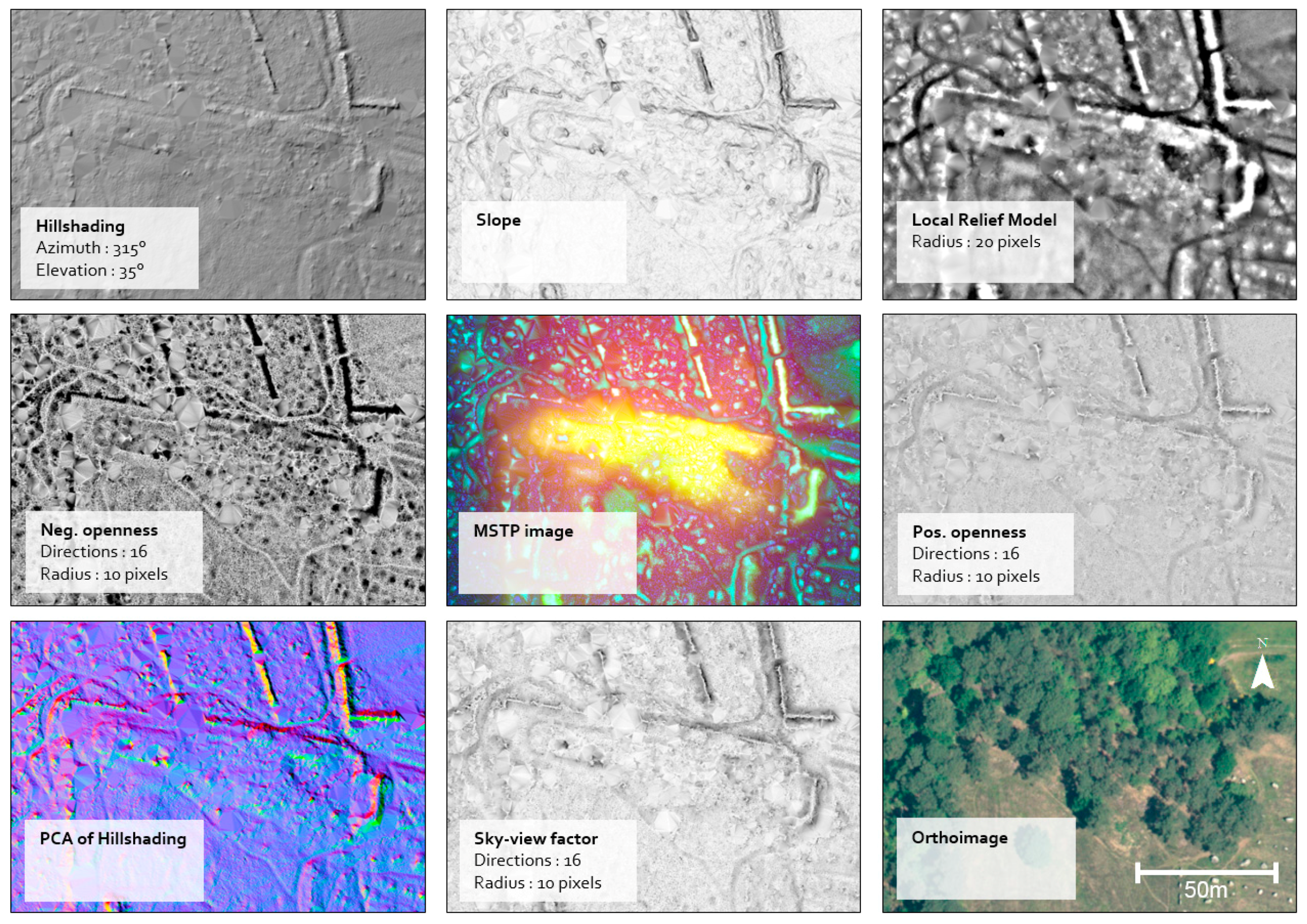
2.3.2. Multi-Scale Topographic Analysis
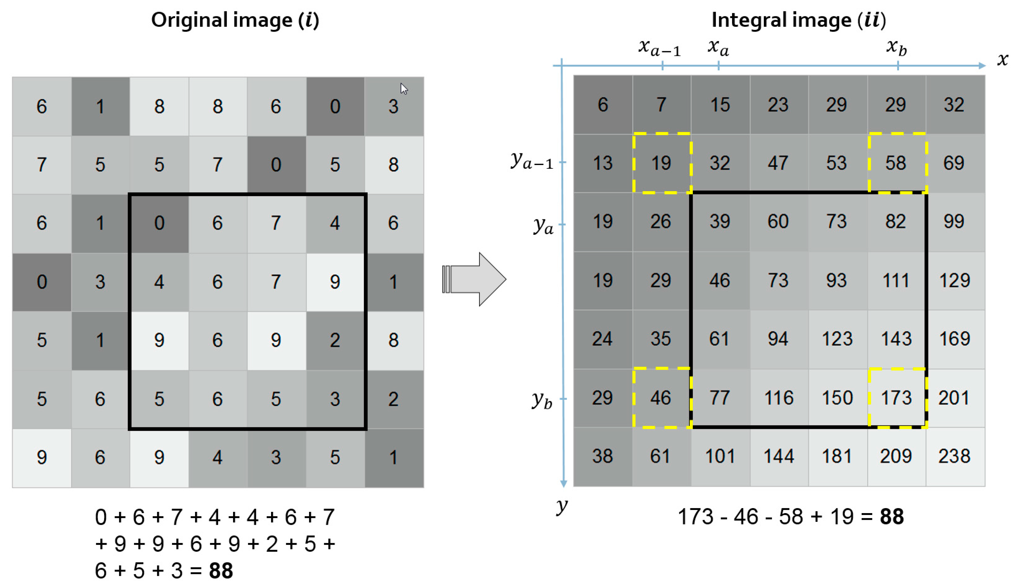
Integral Image Transformation
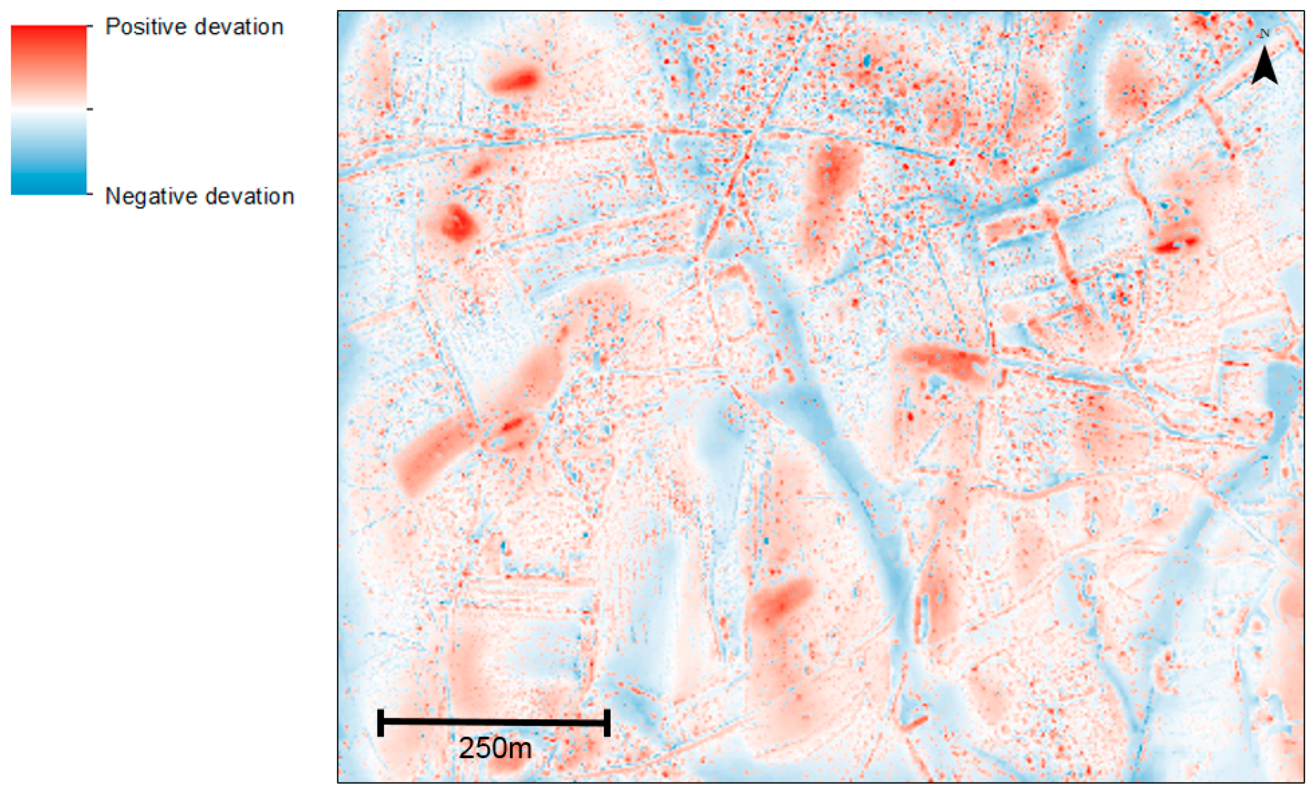
Calculating Topographic Deviation at Multiple Scales
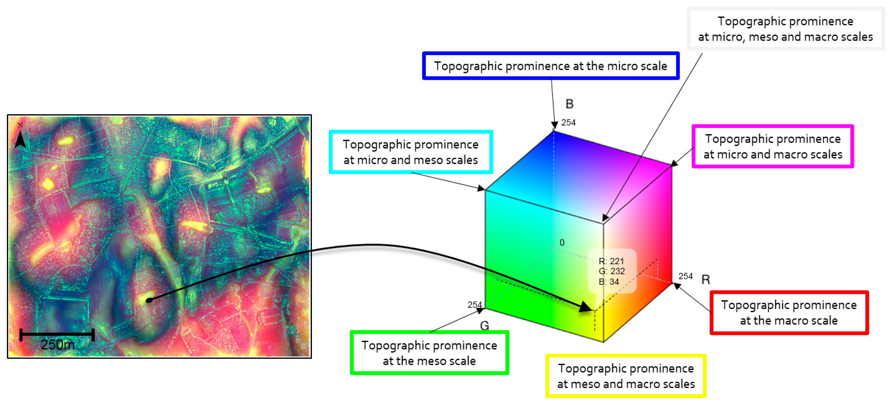
MSTP Image, the Multi-Scale Image Composite
2.3.3. Implementing the Machine Learning Algorithm
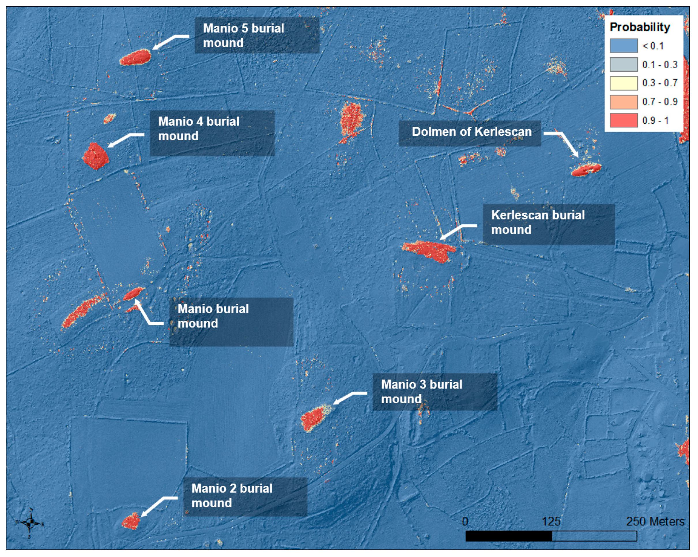
3. Results
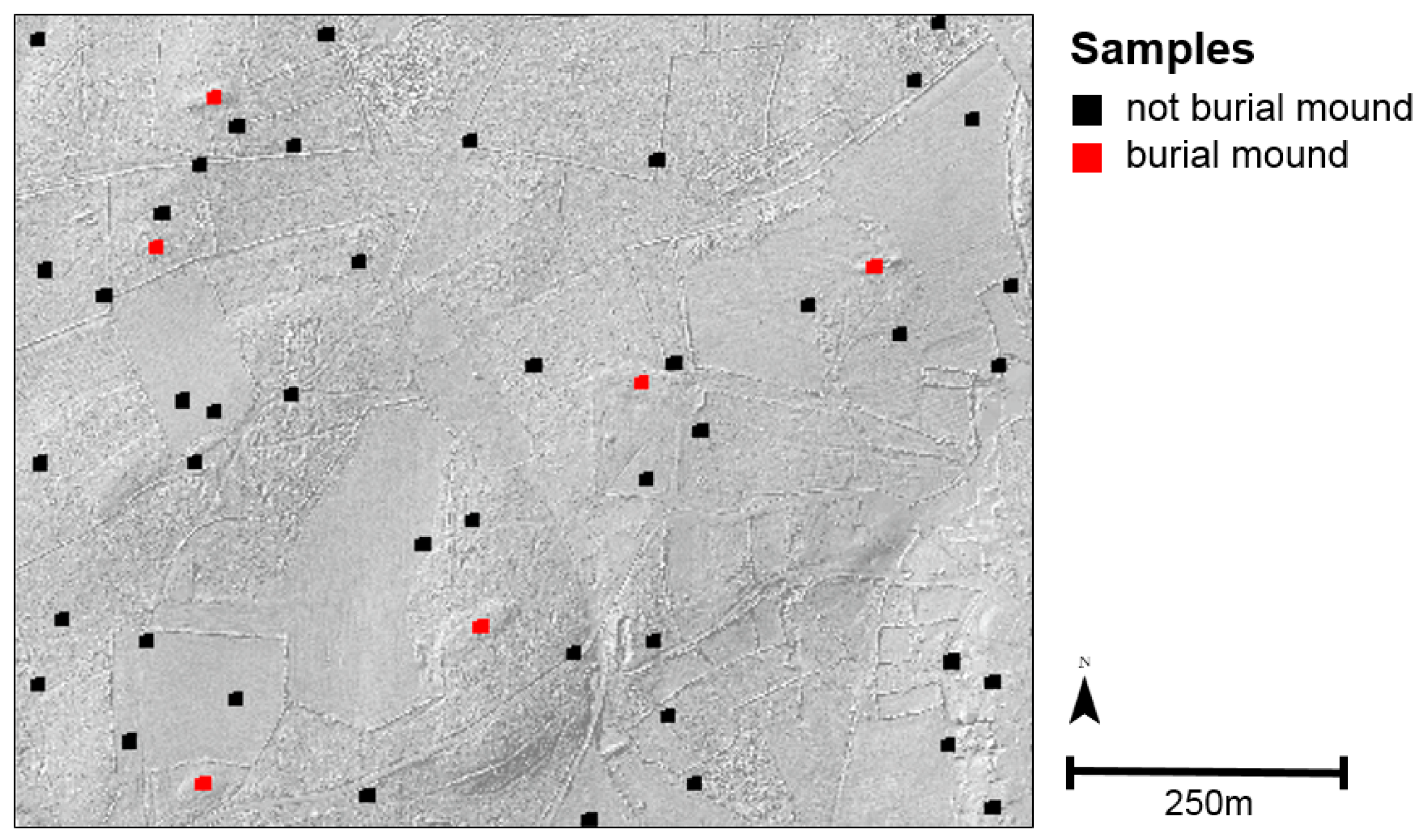
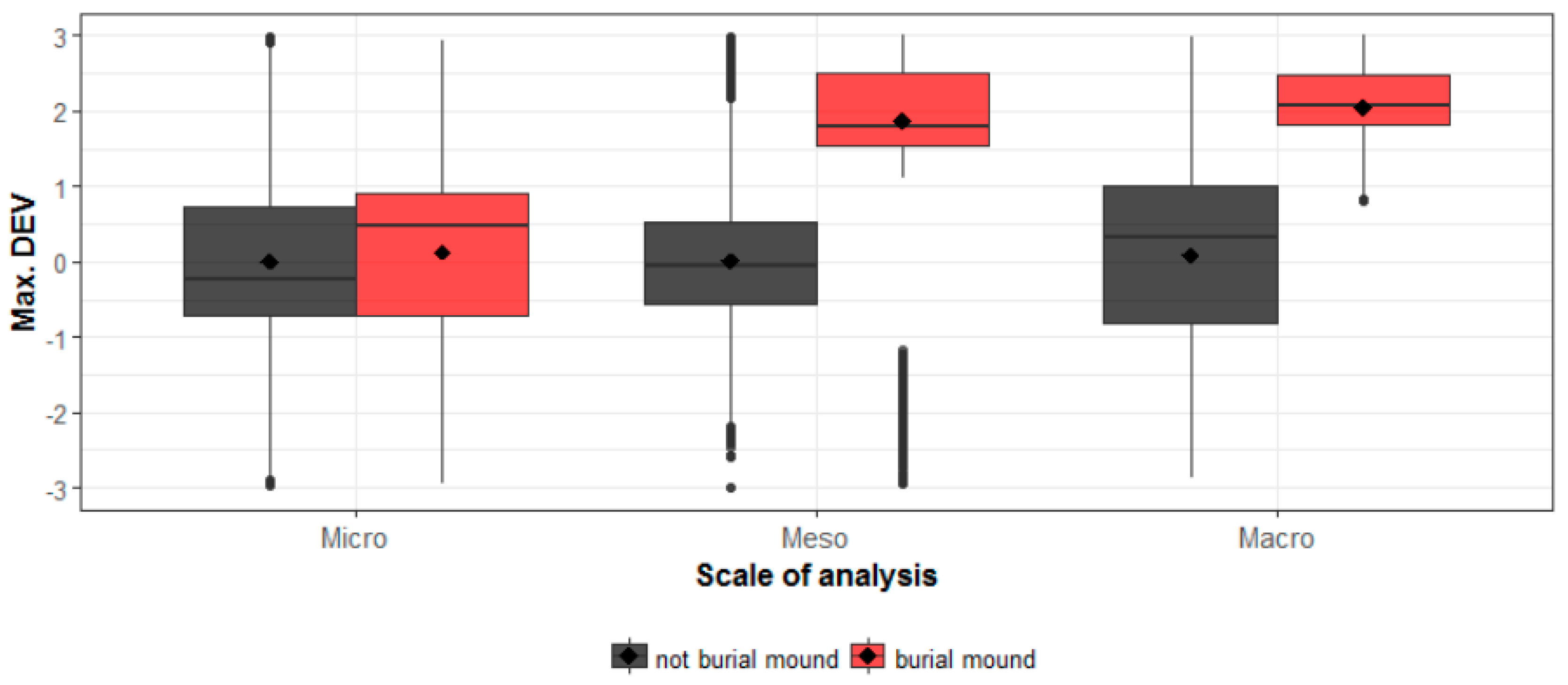
3.1. Training the Model to the Kerlescan Sub-Area
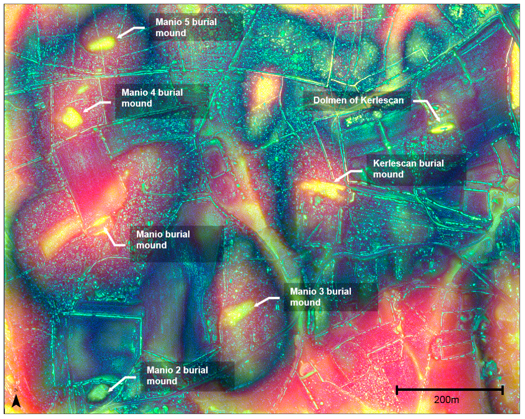
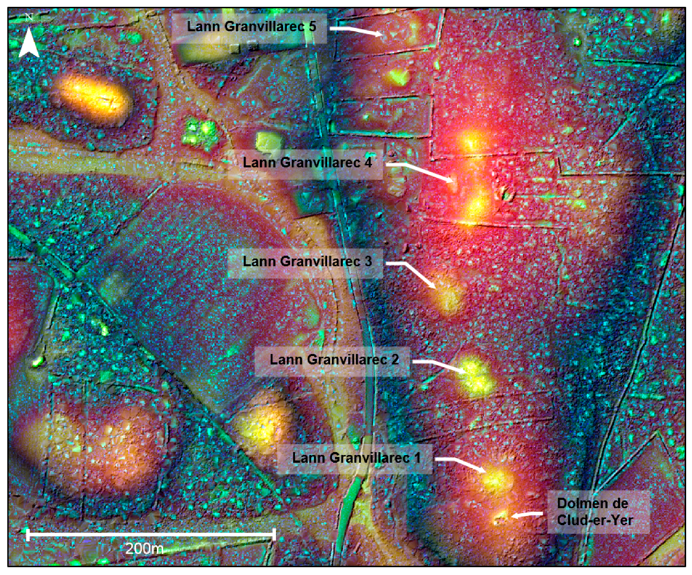
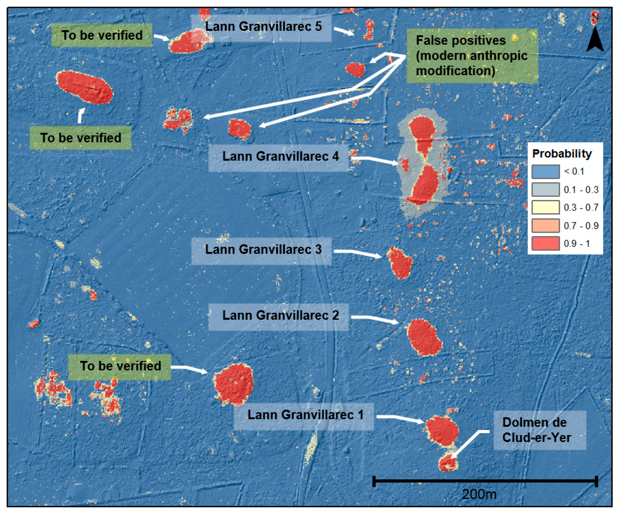
3.2. Applying the Model to the Lann Granvillarec Sub-Area
4. Discussion and Perspectives
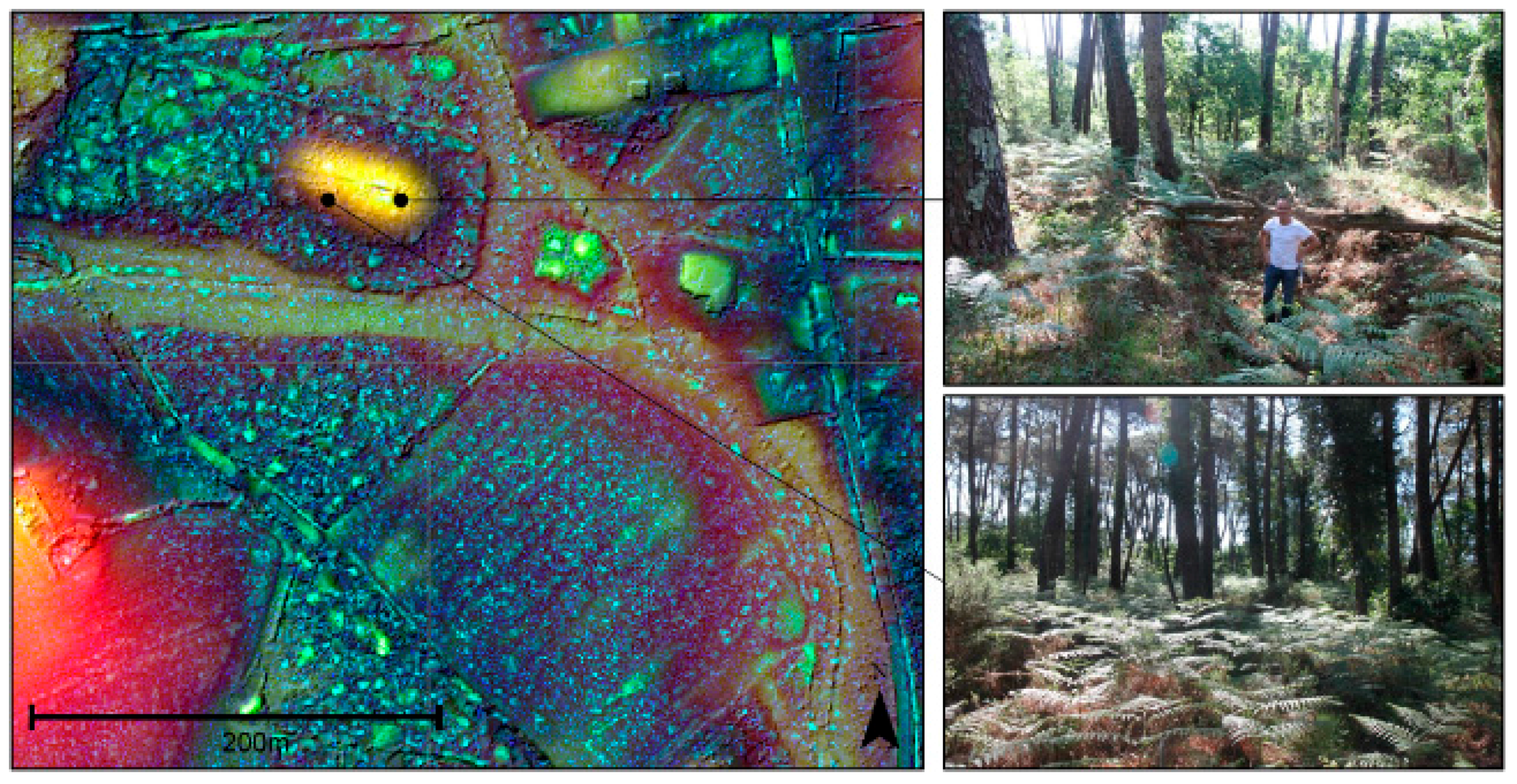
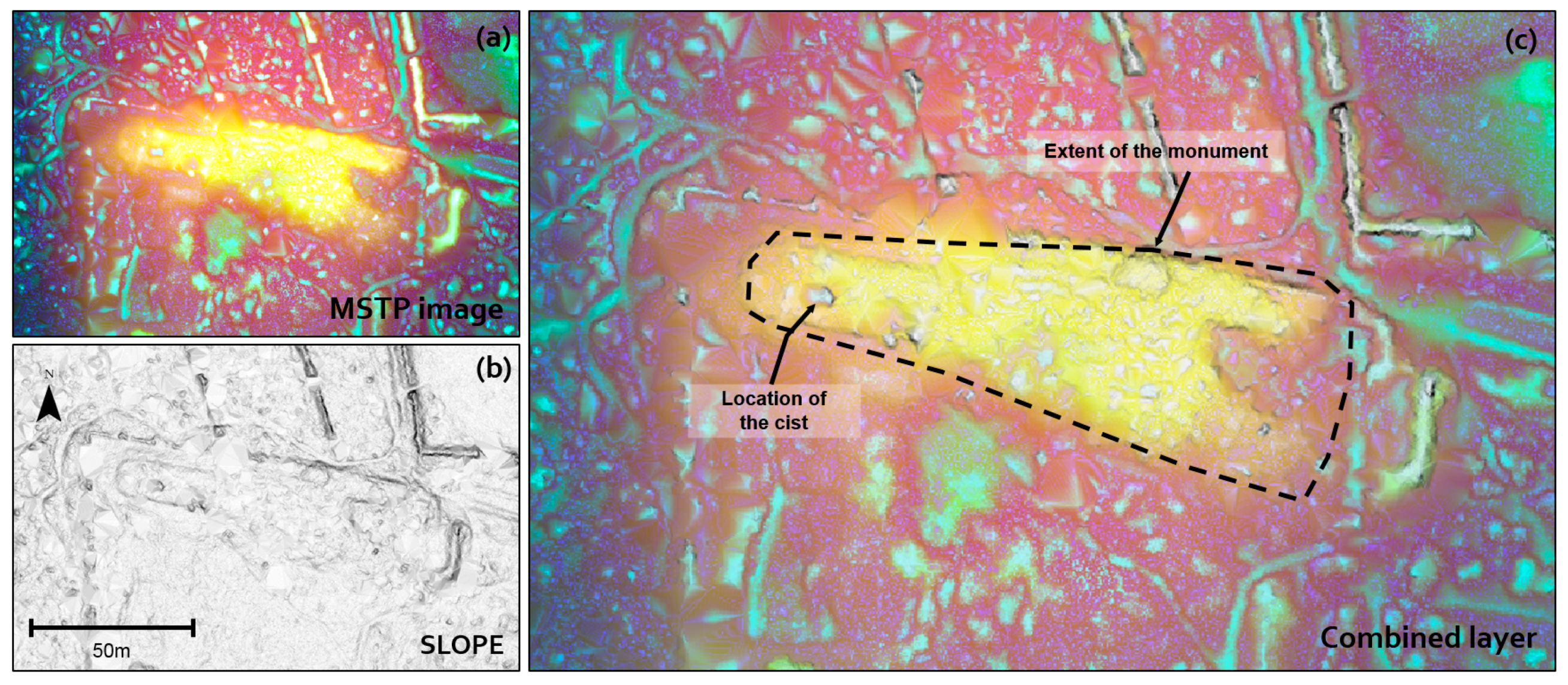
4.1. Comparing MSTP and Other VTs of the Burial Mound of Kerlescan
4.2. Advantages and Limitations of MSTP
4.3. RF Classifier and Futur Perspectives
5. Conclusions
- A pertinent and innovative VT for using a LiDAR-derived DTM in archaeology
- The ability to help archaeologists improve descriptions (geographic location and extent, morphology) of inventoried structures
- A support for archaeological prospection (through visualisation/interpretation of MSTP images)
- A step towards semi-automatic detection by incorporating machine learning (RF) algorithms
Acknowledgments
Author Contributions
Conflicts of Interest
References
- Bewley, R.H. Aerial survey for archaeology. Photogramm. Rec. 2003, 18, 273–292. [Google Scholar] [CrossRef]
- Devereux, B.J.; Amable, G.S.; Crow, P. Visualisation of LiDAR terrain models for archaeological feature detection. Antiquity 2008, 82, 470–479. [Google Scholar] [CrossRef]
- Devereux, B.J.; Amable, G.S.; Crow, P.; Cliff, A.D. The potential of airborne lidar for detection of archaeological features under woodland canopies. Antiquity 2005, 79, 648–660. [Google Scholar] [CrossRef]
- Opitz, R.S.; Cowley, D. (Eds.) Interpreting Archaeological Topography: Airborne Laser Scanning, 3D Data and Ground Observation; Oxbow Books: Oxford, UK; Oakville, CT, USA, 2013. [Google Scholar]
- Freeland, T.; Heung, B.; Burley, D.V.; Clark, G.; Knudby, A. Automated feature extraction for prospection and analysis of monumental earthworks from aerial LiDAR in the Kingdom of Tonga. J. Archaeol. Sci. 2016, 69, 64–74. [Google Scholar] [CrossRef]
- Trier, Ø.D.; Pilø, L.H. Automatic Detection of Pit Structures in Airborne Laser Scanning Data: Automatic detection of pits in ALS data. Archaeol. Prospect. 2012, 19, 103–121. [Google Scholar] [CrossRef]
- Fergusson, J. Rude Stone Monuments in All Countries, Their Age and Uses; John Murray: London, UK, 1872. [Google Scholar]
- Le Rouzic, Z. Les monuments mégalithiques du Morbihan: causes de leur ruine et origine de leur restauration. Bull. Soc. Préhist. Fr. 1939, 36, 234–251. [Google Scholar] [CrossRef]
- Boujot, C.; Vigier, E. Carnac et Environs: Architecture Mégalithiques; Ed. du Patrimoine: Paris, France, 2012. [Google Scholar]
- Roughley, C. The Neolithic Landscape of the Carnac Region, Brittany: New Insights from Digital Approaches. Proc. Prehist. Soc. 2004, 70, 153–172. [Google Scholar] [CrossRef]
- Boujot, C.; Cassen, S. A pattern of evolution for the Neolithic funerary structures of the west of France. Antiquity 1993, 67, 477–491. [Google Scholar] [CrossRef]
- Roughley, C. Understanding the Neolithic landscape of the Carnac region: A GIS approach. BAR Int. Ser. 2001, 931, 211–218. [Google Scholar]
- Bennett, R.; Welham, K.; Hill, R.A.; Ford, A. A Comparison of Visualization Techniques for Models Created from Airborne Laser Scanned Data: A Comparison of Visualization Techniques for ALS Data. Archaeol. Prospect. 2012, 19, 41–48. [Google Scholar] [CrossRef]
- Doneus, M. Openness as Visualization Technique for Interpretative Mapping of Airborne Lidar Derived Digital Terrain Models. Remote Sens. 2013, 5, 6427–6442. [Google Scholar] [CrossRef]
- Kokalj, Ž.; Zakšek, K.; Oštir, K. Application of sky-view factor for the visualisation of historic landscape features in lidar-derived relief models. Antiquity 2011, 85, 263–273. [Google Scholar] [CrossRef]
- Štular, B.; Kokalj, Ž.; Oštir, K.; Nuninger, L. Visualization of lidar-derived relief models for detection of archaeological features. J. Archaeol. Sci. 2012, 39, 3354–3360. [Google Scholar] [CrossRef]
- Zakšek, K.; Oštir, K.; Kokalj, Ž. Sky-View Factor as a Relief Visualization Technique. Remote Sens. 2011, 3, 398–415. [Google Scholar] [CrossRef]
- De Reu, J.; Bourgeois, J.; Bats, M.; Zwertvaegher, A.; Gelorini, V.; De Smedt, P.; Chu, W.; Antrop, M.; De Maeyer, P.; Finke, P.; et al. Application of the topographic position index to heterogeneous landscapes. Geomorphology 2013, 186, 39–49. [Google Scholar] [CrossRef]
- Wilson, J.P.; Gallant, J.C. (Eds.) Terrain Analysis: Principles and Applications; Wiley: New York, NY, USA, 2000. [Google Scholar]
- Lindsay, J.B.; Cockburn, J.M.H.; Russell, H.A.J. An integral image approach to performing Multi-Scale Topographic Position analysis. Geomorphology 2015, 245, 51–61. [Google Scholar] [CrossRef]
- Kotsiantis, S.B.; Zaharakis, I.; Pintelas, P. Supervised Machine Learning: A Review of Classification Techniques; IOS Press: Amsterdam, The Netherlands, 2007. [Google Scholar]
- Breiman, L. Random forests. Mach. Learn. 2001, 45, 5–32. [Google Scholar] [CrossRef]
- Pal, M. Random forest classifier for remote sensing classification. Int. J. Remote Sens. 2005, 26, 217–222. [Google Scholar] [CrossRef]
- Kokalj, Ž.; Zaksek, K.; Oštir, K.; Pehani, P.; Čotar, K. Relief Visualization Toolbox, Version 1.3, Manual; Research Centre of the Slovenian Academy of Sciences and Arts: Ljubljana, Slovenia, 2016; Available online: https://iaps.zrc-sazu.si/en/rvt#v (accessed on 22 December 2017).
- Isenburg, M. Efficient LiDAR Processing Software; Rapidlasso: Gilching, Germany, 2017; Available online: http://rapidlasso.com/lastools/ (accessed on 22 December 2017).
- Georges-Leroy, M.; Nuninger, L.; Opitz, R. Le lidar: Une Technique de Détection au Service de L’archéologie. 2014. Available online: https://hal.archives-ouvertes.fr/halshs-01099797 (accessed on 22 December 2017).
- Lindsay, J.B. The Whitebox Geospatial Analysis Tools project and open-access GIS. Unpublished work. 2014. [Google Scholar]
- R Core Team. R: A Language and Environment for Statistical Computing; R Foundation for Statistical Computing: Vienna, Austria, 2013. [Google Scholar]
- Crow, F.C. Summed-area tables for texture mapping. ACM SIGGRAPH Comput. Graph. 1984, 18, 207–212. [Google Scholar] [CrossRef]
- Kuhn, M.; Wing, J.; Weston, S.; Williams, A.; Keefer, C.; Engelhardt, A.; Cooper, T.; Mayer, Z.; Kenkel, B.; The R Core Team; et al. Caret: Classification and Regression Training. 2017. Available online: https://cran.r-project.org/package=caret (accessed on 22 December 2017).
- McKay, M.D.; Beckman, R.J.; Conover, W.J. Comparison of Three Methods for Selecting Values of Input Variables in the Analysis of Output from a Computer Code. Technometrics 1979, 21, 239–245. [Google Scholar]
- Cohen, J. A Coefficient of Agreement for Nominal Scales. Educ. Psychol. Meas. 1960, 20, 37–46. [Google Scholar] [CrossRef]
- Zeugmann, T.; Poupart, P.; Kennedy, J.; Jin, X.; Han, J.; Saitta, L.; Sebag, M.; Peters, J.; Bagnell, J.; Daelemans, W.; et al. Precision and Recall. In Encyclopedia of Machine Learning; Sammut, C., Webb, G.I., Eds.; Springer: Boston, MA, USA, 2011; p. 781. [Google Scholar]
- Caruana, R.; Niculescu-Mizil, A. An empirical comparison of supervised learning algorithms. In Proceedings of the 23rd International Conference on Machine Learning, Pittsburgh, PA, USA, 25–29 June 2006; pp. 161–168. [Google Scholar]
- Fernández-Delgado, M.; Cernadas, E.; Barro, S.; Amorim, D. Do we need hundreds of classifiers to solve real world classification problems. J. Mach. Learn. Res. 2014, 15, 3133–3181. [Google Scholar]
- Krizhevsky, A.; Sutskever, I.; Hinton, G.E. Imagenet classification with deep convolutional neural networks. In Advances in Neural Information Processing Systems; ACM: New York, NY, USA, 2012; pp. 1097–1105. [Google Scholar]
- Zhang, L.; Zhang, L.; Du, B. Deep Learning for Remote Sensing Data: A Technical Tutorial on the State of the Art. IEEE Geosci. Remote Sens. Mag. 2016, 4, 22–40. [Google Scholar] [CrossRef]
- Geng, J.; Fan, J.; Wang, H.; Ma, X.; Li, B.; Chen, F. High-Resolution SAR Image Classification via Deep Convolutional Autoencoders. IEEE Geosci. Remote Sens. Lett. 2015, 12, 2351–2355. [Google Scholar] [CrossRef]


| Survey Parameter | Value |
|---|---|
| Area covered | 246.7 km2 |
| Flight altitude | 1300 m above ground level |
| LiDAR mode | Multi-echo (up to 5 returns) |
| Laser wavelengths (nm) | 1064 nm (near-infrared), 532 nm (green) |
| Beam divergence | 0.35 mrad (near-infrared), 0.7 mrad (green) |
| Scan frequency | 61 Hz |
| Pulse repetition frequency | 300 kHz |
| Field of view | 26° [13°; +13°] |
| Absolute vertical accuracy | 8 cm |
| Absolute horizontal accuracy | 12 cm |
| Total number of 3D points acquired | 5.2 billion |
| Nominal point density | 14 points/m2 |
| Window Size Range [] | ||
|---|---|---|
| Scale | In metres | In pixels (0.25 m resolution) |
| micro | [1; 10] | [3 × 3; 41 × 41] |
| meso | [10; 100] | [41 × 41; 401 × 401] |
| macro | [100; 1000] | [ 401 × 401; 4001 × 4001] |
| Predicted “Not Burial Mound” | Predicted “Burial Mound” | |
|---|---|---|
| Actual “not burial mound” | 22,126 | 41 (fp) |
| Actual “burial mound” | 46 (fn) | 2952 (tp) |
© 2018 by the authors. Licensee MDPI, Basel, Switzerland. This article is an open access article distributed under the terms and conditions of the Creative Commons Attribution (CC BY) license (http://creativecommons.org/licenses/by/4.0/).
Share and Cite
Guyot, A.; Hubert-Moy, L.; Lorho, T. Detecting Neolithic Burial Mounds from LiDAR-Derived Elevation Data Using a Multi-Scale Approach and Machine Learning Techniques. Remote Sens. 2018, 10, 225. https://doi.org/10.3390/rs10020225
Guyot A, Hubert-Moy L, Lorho T. Detecting Neolithic Burial Mounds from LiDAR-Derived Elevation Data Using a Multi-Scale Approach and Machine Learning Techniques. Remote Sensing. 2018; 10(2):225. https://doi.org/10.3390/rs10020225
Chicago/Turabian StyleGuyot, Alexandre, Laurence Hubert-Moy, and Thierry Lorho. 2018. "Detecting Neolithic Burial Mounds from LiDAR-Derived Elevation Data Using a Multi-Scale Approach and Machine Learning Techniques" Remote Sensing 10, no. 2: 225. https://doi.org/10.3390/rs10020225