Classification of Hyperspectral Images by SVM Using a Composite Kernel by Employing Spectral, Spatial and Hierarchical Structure Information

Abstract

In this paper, we introduce a novel classification framework for hyperspectral images (HSIs) by jointly employing spectral, spatial, and hierarchical structure information. In this framework, the three types of information are integrated into the SVM classifier in a way of multiple kernels. Specifically, the spectral kernel is constructed through each pixel’s vector value in the original HSI, and the spatial kernel is modeled by using the extended morphological profile method due to its simplicity and effectiveness. To accurately characterize hierarchical structure features, the techniques of Fish-Markov selector (FMS), marker-based hierarchical segmentation (MHSEG) and algebraic multigrid (AMG) are combined. First, the FMS algorithm is used on the original HSI for feature selection to produce its spectral subset. Then, the multigrid structure of this subset is constructed using the AMG method. Subsequently, the MHSEG algorithm is exploited to obtain a hierarchy consist of a series of segmentation maps. Finally, the hierarchical structure information is represented by using these segmentation maps. The main contributions of this work is to present an effective composite kernel for HSI classification by utilizing spatial structure information in multiple scales. Experiments were conducted on two hyperspectral remote sensing images to validate that the proposed framework can achieve better classification results than several popular kernel-based classification methods in terms of both qualitative and quantitative analysis. Specifically, the proposed classification framework can achieve 13.46–15.61% in average higher than the standard SVM classifier under different training sets in the terms of overall accuracy.

1. Introduction

With the rapid development of hyperspectral sensors, the present hyperspectral images (HSIs) contain rich spectral and spatial information. Therefore, different objects can be accurately recognized from HSIs using various classification algorithms for different applications, such as geological survey [1], mineral mapping [2], fine agricultural research [3,4], environmental monitoring [5], etc.

HSI classification is one of the most popular problems in the field of remote sensing and has aroused much concern, but faces the following challenges [6,7,8]: First, it is very difficult to acquire sufficient labeled samples. Second, information redundancy and Hughes phenomenon are inevitable due to the high dimensional features represented by hundreds of spectral bands. Finally, HSIs are often corrupted with different types of noise and dominated by mixed pixels. To solve these problems, many researchers recurred to pixel-wise methods to classify each pixel in HSIs to a certain class using its spectral information individually [9,10,11,12,13,14]. Among them, the SVM [10,15] and multinomial logistic regression (MLR) [16,17,18] are the two most commonly used techniques. However, these methods often result in much “salt-and-pepper” noise in classification maps, without considering spatial neighborhoods, and the classification performance cannot be further improved.

This difficulty has been greatly conquered at the appearance of spectral-spatial classification methods [19]. Generally, these methods can be divided into three categories. In the first category, spatial information is integrated with spectral information by using composite kernels [20,21,22,23]. There are many methods for spatial feature extraction, such as mean filtering [20], area filtering [24], Gabor filtering [25], gray-level co-occurrence matrix [26], edge-preserving filtering (EPF) [27], and extended morphological profiles (EMPs) [28]. In the second category, the integration of the spectral information and the spatial information is first performed by image segmentation algorithms, such as mean-shift [29], watershed [30], hierarchical segmentation [31,32], minimum spanning forest [33], graph cut [34,35], and superpixel [36] approaches. Then, the final classification map is produced by combining the pixel-wise classification map and the unsupervised segmentation map by employing a majority voting algorithm. In the third category, the two types of information are jointly included in the classification process using Markov random field (MRF) models. By applying the maximum a posteriori (MAP) decision rule, HSI classification can be effectively solved by minimizing a MAP-MRF energy function. The ensemble method of SVM and the MRF-based model is a regular scheme [37,38,39,40,41,42,43].

Kernel-based classification methods have been very popular for HSI classification because they can effectively deal with the intractable issues of curse of dimensionality, limited labeled samples, and noise corruption. The SVM algorithm using a single (e.g., linear, polynomial, or Gaussian radial basis function (RBF)) kernel has been widely used for image classification. To perform HSI classification, several SVM techniques using the spectral-spatial kernel were presented. For instance, Camps-Valls et al. [20] formulated a general framework of multiple kernels by exploring both the spectral and spatial information, and the spatial information is defined using basic statistical measures within a fixed-size window in the image. The selection of a suitable window size is a challenging problem because spatial structures extracted from such a region cannot be accurately represented. To solve this problem, the adaptive neighborhood system based on morphological filtering and area filtering has been considered. On the one hand, Fauvel et al. [44] applied feature extraction on the original HSI and its EMPs, respectively, and performed the SVM classification using the RBF kernel with spectral-spatial stacked vectors. Li et al. [45] developed a MLR framework using generalized composite kernels (GCK), where the spatial information is represented by using EMPs as well. The obtained spatial information by such methods is highly dependent to the Structuring Element (SE) of morphological operators. On the other hand, Fauvel et al. [22] proposed an improved SVM by using a customized spectral-spatial kernel where the spatial information is modeled as the median value on the adaptive neighbourhood of each pixel defined using morphological area filtering. The result that is achieved by such a method is very sensitive to the predefined number of areas. Recently, the superpixel-based techniques have been applied to HSI classification by Shutao Li’s research group. Fang et al. [46] presented an effective SVM classifier characterized with a superpixel-based composite kernel, where the three types of the spectral, intra-superpixel and inter-superpixel information are combined, and the superpixel map is obtained using the entropy rate superpixel (ERS) algorithm. Meanwhile, texture features are crucial for object classification of HSIs. Later, we introduced an alternative SVM classifier featured with a spectral-texture kernel [23], where the textual information is modeled for each superpixel with its local spectral histogram. The number of superpixels is a data-dependent and greatly influences classification results. Lu et al. [47] developed an effective HSI classification framework by integrating the multiple feature-induced kernels into a SVM classifier, where subpixel, pixel and superpixel features are combined. More recently, Peng et al. [48] improved the spectral-spatial composite kernel by embedding label information with an ideal regularized technique. The information that is extracted from the label domain cannot describe spatial structures well.

In this paper, we develop a novel SVM classification framework with the spectral, spatial, and hierarchical kernels (SVM-SSHK), in which the spectral, spatial, and hierarchical structure information in HSIs are integrated into the SVM classifier in a way of multiple kernels. Specifically, the spectral kernel is constructed through each pixel’s vector value in the original HSI, and the spatial kernel is modeled by using the EMP method due to its simplicity and effectiveness. To accurately characterize hierarchical structure features, the techniques of Fish-Markov selector (FMS), marker-based hierarchical segmentation (MHSEG) and algebraic multigrid (AMG) are combined. First, the FMS algorithm is used on the original image for feature selection to produce its spectral subset. Then, the multigrid structure of this subset is constructed using the AMG method. Subsequently, the MHSEG algorithm is exploited to obtain a hierarchy consisting of a series of segmentation maps. Finally, the hierarchical structure information is modeled by using these segmentation maps. The main contributions of this work is to present an effective composite kernel framework for HSI classification by utilizing spatial structure information in multiple scales. The previously mentioned kernel-based approaches cannot simultaneously capture salient and fine structures in the image with a predefined number of regions. However, the proposed framework can obtain a hierarchical representation of spatial structure information in HSIs. Furthermore, this hierarchical structure is only dependent to the original HSI, without considering the problem of choosing a neighborhood system or the size of a region (e.g., an area or a superpixel).

The remainder of the paper is organized as follows. In Section 2, some related techniques are reviewed. In Section 3, the proposed classification framework that is characterized with a spectral-spatial-hierarchical kernel is introduced. In Section 4, experimental results are reported in comparing to popular HSI classification methods and some issues are discussed. The last section presents some concluding remarks and the future work.

2. Related Techniques

Let x represent an HSI which contains B-band vectors with $x\equiv \left\{x_1,x_2,\dots ,x_N\right\}\in {ℝ}^B$, $\mathbf{y}\equiv \left\{y_1,y_2,\dots ,y_N\right\}\in L^N$ the final classification result with $y_k\equiv \left\{L_1,L_2,\dots ,L_T\right\}$ ($k=1,2,\dots ,N$), ${\left\{\left(x_k,y_k\right)\right\}}_{k=1}^n$ training samples, $n_i$ the number of the training samples of $L_i$ ($i=1,2,\dots ,Z$).

2.1. Spatial Information with EMPs

In the spectral-spatial classification method, the first step is to extract some featured bands to model spectral information from hyperspectral images (HSIs) by dimensionality reduction, which is used to minimize redundant information and to improve computational efficiency. To this end, the most popular approaches have been used, such as principal component analysis (PCA) [28], independent component analysis (ICA) [49], Kernel PCA [50], decision boundary feature extraction, nonparametric weighted feature extraction, and Bhattacharyya distance feature selection [51]. In this work, the widely used PCA transform was used to produce the EMP. First, almost all of the spectral information in HSIs can be represented by using the first three or four principal components (PCs). Second, object boundaries in the HSIs can be better preserved in the resultant PCs [27]. Finally, it was recorded that the EMP was first constructed using PCA [7].

The main idea of EMP is to reconstruct the spatial information through morphological (opening/closing) operators, while preserving the boundaries of the image. Let k and n be the total number of the selected principal components (PCs) and the morphological operators, respectively, ψ and η the opening and closing operations, and I a gray-level image, we can build the morphological profile (MP) for each PC, as follows:

$$MP\left(I\right)=\left\{{\psi }_{\mathrm{T}}\left(I\right),\dots ,{\psi }_2\left(I\right),{\psi }_1\left(I\right),I,{\eta }_1\left(I\right),{\eta }_2\left(I\right),\dots ,{\eta }_{\mathrm{T}}\left(I\right)\right\}$$

(1)

For each PC, the MP is a (2n + 1)-band image. Then, the MPs are stacked to obtain the EMP as follows:

$$EM{P}_k=\left\{MP\left(P{C}_1\right),MP\left(P{C}_2\right),\dots ,MP\left(P{C}_k\right)\right\}.$$

(2)

where EMP is a stacked vector with the dimensionality of $k\left(2n+1\right)$ and includes both the spectral and spatial information of the HSIs. In fact, we can extract EMPs for all of the spectral bands or for some selective bands in the HSIs without PCA, which causes the following limitations. First, some redundancy can be observed in the $B\left(2n+1\right)$-band image, where B is the number of spectral bands for the HSI, which may decrease the classification accuracies. Second, the classification process should be fit for such high-dimensional data with much more computational cost.

2.2. Band Selection with FMS

In many research fields, it is necessary for supervised classification to perform feature selection. Given a set of test samples, the selected features are used to assign a class label for each sample. Feature selection and subspace methods are widely used for dimensionality reduction [52,53,54,55]. For instance, Cheng et al. [56] presented the FMS algorithm for the feature selection of high-dimensional data, whose basic idea is to find the optimal subset of features to maximize intra-class separability and minimize inter-class variations in a higher dimensional kernel space. By employing some spectral kernel functions, such as the polynomial kernel, the feature selection problem can be solved efficiently using MRF optimization techniques. In the original space, denote the within-, between- (or inter-) class, and total scatter matrices by $S_w$, $S_b$, and $S_t$:

$$S_w=\frac{1}{N}{\displaystyle \sum _{j=1}^Z{\displaystyle \sum _{i=1}^{n_j}\left(x_i^{\left(j\right)}-m_j\right){\left(x_i^{\left(j\right)}-m_j\right)}^T}}$$

(3)

$$S_b=\frac{1}{N}{\displaystyle \sum _{j=1}^Z{n}_j\left(m_j-m\right){\left(m_j-m\right)}^T}$$

(4)

$$S_t=\frac{1}{N}{\displaystyle \sum _{i=1}^n{n}_j\left(x_i-m\right){\left(x_i-m\right)}^T}=S_w+S_b$$

(5)

where $x_i^{\left(j\right)}$ is the ith training sample in class $L_j$, and $m_j$ and $m$ represent the sample means for class $L_j$ and the whole training set, respectively. The scatter matrices are denoted by ${\tilde{S}}_w$, ${\tilde{S}}_b$, and ${\tilde{S}}_t$ in the kernel space, whose traces in algebra can be calculated as follows:

$$\mathrm{Tr}({\tilde{S}}_w)=\frac{1}{n}\mathrm{Tr}\left(K\right)-{\displaystyle \sum _{i=1}^Z\frac{1}{n_i}\mathrm{Sum}\left(K^{\left(i\right)}\right)}$$

(6)

$$\mathrm{Tr}({\tilde{S}}_b)=\frac{1}{n}{\displaystyle \sum _{i=1}^Z\frac{1}{n_i}}\mathrm{Sum}\left(K^{\left(i\right)}\right)-\frac{1}{n^2}\mathrm{Sum}\left(K\right)$$

(7)

$$\mathrm{Tr}({\tilde{S}}_t)=\frac{1}{\mathrm{n}}\mathrm{Tr}\left(K\right)-\frac{1}{n^2}\mathrm{Sum}\left(K\right)$$

(8)

where $\mathrm{Tr}(\cdot )$ and $\mathrm{Sum}(\cdot )$ are the summation and trace operators, respectively, and $K$ and $K^{\left(i\right)}$ are two matrices with size of $n\times n$ and $n_i\times n_i$, respectively, and have the following forms:

$${\left\{K\right\}}_{k,l}=k\left(x_k,x_l\right), k,l\in \left\{1,2,\dots ,n\right\}$$

(9)

$${\left\{K^{\left(i\right)}\right\}}_{u,v}=k\left(x_u^{\left(i\right)},x_v^{\left(i\right)}\right), u,v\in \left\{1,2,\dots ,n_i\right\}, i=1,2,\dots ,Z$$

(10)

The feature selector is represented by $\alpha ={\left[{\alpha }_1,{\alpha }_2,\dots ,{\alpha }_B\right]}^Z\in {\left\{0,1\right\}}^B$, where “1” indicates that the kth feature is selected or “0” not selected. The selected features from the vector x are defined, as follows:

$$x\left(\alpha \right)=x\odot \alpha$$

(11)

where $\odot$ is the Hadamard product. Substituting (9) and (10) with (11), $K$ and $K^{\left(i\right)}$ can be expressed as functions of α:

$${\left\{K\left(\alpha \right)\right\}}_{k,l}=k\left(x_k\odot \alpha ,x_l\odot \alpha \right)$$

(12)

$${\left\{K^{\left(i\right)}\left(\alpha \right)\right\}}_{u,v}=k\left(x_u^{\left(i\right)}\odot \alpha ,x_v^{\left(i\right)}\odot \alpha \right)$$

(13)

In such way, the previously mentioned scatter matrices can be defined as functions of α as $\mathrm{Tr}\left({\tilde{S}}_w\left(\alpha \right)\right)$, $\mathrm{Tr}\left({\tilde{S}}_b\left(\alpha \right)\right)$ and $\mathrm{Tr}\left({\tilde{S}}_t\left(\alpha \right)\right)$.

The aim of feature selection is to maximize the class separations for the most discriminative capability of the variables. According to the spirit of Fisher, the following optimization function can be obtained:

$$\underset{\alpha \in {\left\{0,1\right\}}^B}{\arg \max }\left\{\mathrm{Tr}\left({\tilde{S}}_b\right)\left(\alpha \right)-\lambda \mathrm{Tr}\left({\tilde{S}}_t\right)\left(\alpha \right)\right\}$$

(14)

where λ is a parameter to balance the two items.

Actually, Equation (14) is a special case of the Markov problem without pairwise interaction term and can result in the optimal solution. In this work, we can compute a coefficient for each band of HSIs to demonstrate its significance by using the FMS algorithm. The higher the coefficient, the more significant the corresponding band. In this way, we can obtain the most relevant spectral bands.

2.3. Hierarchical Representation of HSIs

To construct a scale-space representation of a HSI $\mathbf{u}=\left[u_1,u_2,\dots ,u_N\right]$, a vector-valued anisotropic diffusion PDE can be used [57,58]:

$$\frac{\partial u_i}{\partial t}=\mathrm{div}\left(g\left(\theta \left(\nabla {\mathbf{u}}_{\sigma }\right)\right)\nabla u_i\right), i=1,2,\dots ,N$$

(15)

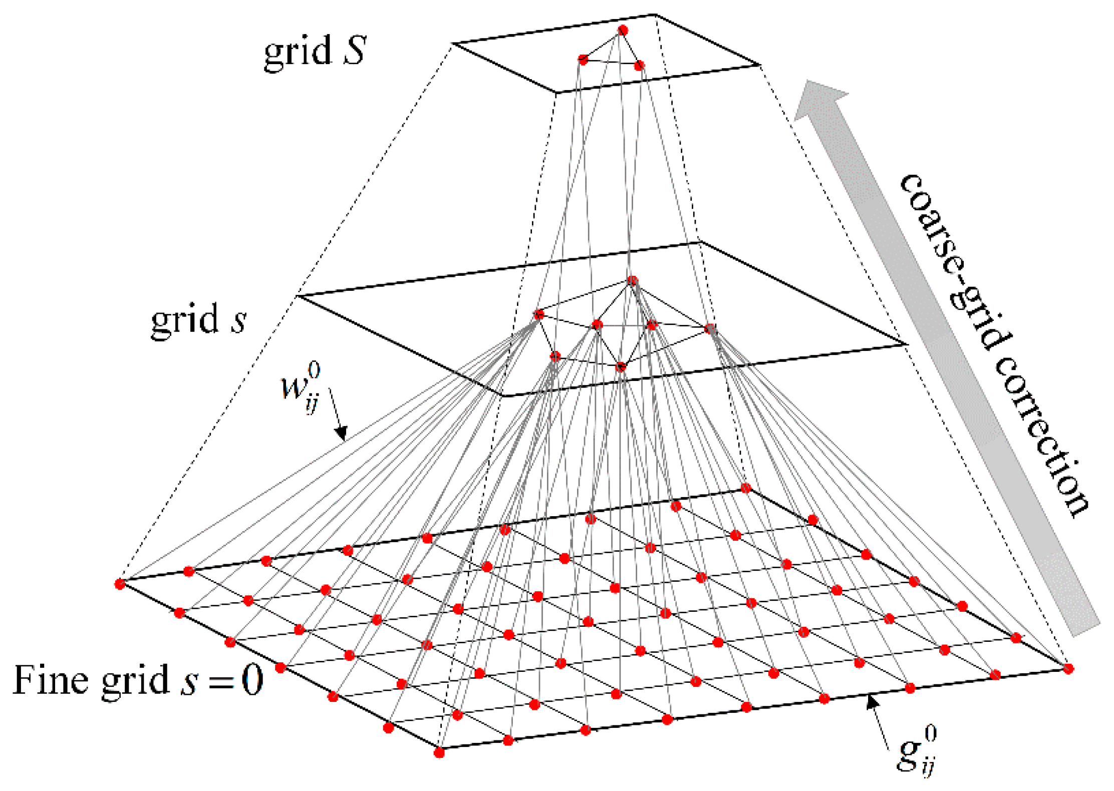
where ${\mathbf{u}}_{\sigma }$ is obtained by convolving u with a Gaussian kernel of standard deviation σ, and $g(\cdot )$ is the diffusivity of $\left|\nabla {\mathbf{u}}_{\sigma }\right|$. Recently, AMG has been used for multiscale representation of HSIs due to the advantage that AMG is capable of constructing a hierarchical representation of the problem from a fine grid to a coarse grid and the linear system is suitable to be effectively solved in the coarsest grid [59]. In this work, the proposed framework exploits all of the vertices in the multigrid structure as the markers.

According to the work of [60], we can construct a “pyramid” multigrid structure of HSIs as shown in Figure 1, where each grid, $s=1,2,\dots ,S$, can be described by a weighted graph $(V^s,E^s)$ in which $V^s$ and $E^s$ are the set of vertices and edges, respectively, and the weight $g_{ij}$ of $\left(i,j\right)\subset E^s$ expresses the similarity between the pixels of $u_i^s$ and $u_j^s$ in $V^s$. Initially, the first graph $(V^0,E^0)$ is built from the original HSI, where $V^0$ denotes the set of vertices, whose size is the same as the HSI, while $E^0$ represents the set of edges connecting each vertex to its four-neighborhoods with weights. In our method, the initial weights $g_{ij}^0$ of $\left(i,j\right)\subset E^0$ are computed by using the diffusivity of the anisotropic diffusion partial differential equation:

$$g\left(\theta \right)=\{\begin{array}{ll}1,\hfill & \theta =0\hfill \\ 1-e^{-\frac{3.31488}{{\left(\theta /\beta \right)}^8}},\hfill & \theta >0\hfill \end{array}$$

(16)

where θ is an indicator of the image edge strength using the Euclidean distance (ED) or the spectral angle mapper (SAM) between two pixel vectors, β denotes a gradient threshold.

The main steps of building the multigrid structure is summarized as follows [60].

Step 1: To consecutively select a new set of $V^{l+1}$ from $V^l$. To build the AMG multigrid structure, the authors of [60] introduced a mass $m_i$ for each vertex, which is a measure for the number of pixels that are assigned to a given vertex selected to the next grid and can be initialized as $m_i^0=1$. The first vertex of $V^{l+1}$ is selected as the vertex in $V^l$ with the greatest mass. The rest vertices in $V^l$ are sorted in decreasing order of mass. Then, a new vertex is iteratively selected if this satisfies the condition as follows [10]:

$$\frac{{\displaystyle \sum _{j\in V^{l+1}}{g}_{ij}^l}}{{\displaystyle \sum _{\left(i,j\right)\in E^l}{g}_{ij}^l}}\le \upsilon \Rightarrow V^{l+1}=V^{l+1}\cup \left\{i\right\}, \mathrm{for} \mathrm{each} i\in V^l\backslash V^{l+1}$$

(17)

where $\upsilon$ is a threshold value with $0\le \upsilon \le 1$, and $V^l\backslash V^{l+1}$ indicates the set difference between $V^l$ and $V^{l+1}$. In the multigrid structure, each vertex has a mass value and the masses in the $\left(l+1\right)$th grid are calculated as follows:

$$\forall i\in V^{l+1}:m_i^{l+1}=m_i^l+{\displaystyle \sum _{j\in V^{l+1}}{w}_{ij}^l}$$

(18)

where $m_i^l$ and $m_i^{l+1}$ are the masses in the lth and $(l+1)$th grids, respectively, and $w_{ij}^l$ weights how much vertex $i\in V^l\backslash V^{l+1}$ depends on the vertex $j\in V^{l+1}$:

$$\forall i\in V^l\backslash V^{l+1},j\in V^{l+1}:w_{ij}^l=w_{ji}^l=\frac{g_{ij}^l}{{\displaystyle \sum _{k\in V^{l+1}}{g}_{ik}^l}}$$

(19)

Step 2: To connect the vertices in $V^{l+1}$ to obtain $E^{l+1}$. The matrix of diffusivities are obtained using the Garlekin operator ${\mathbf{G}}^{l+1}=I_f^c{\mathbf{G}}^l{I}_c^f$ [61], where $I_f^c$ and $I_c^f$ denote the restriction and interpolation operators:

$${\left[I_f^c\right]}_{ij}=\frac{w_{ij}^l}{1+{\displaystyle \sum _{j\in V^l\backslash V^{l+1}}{w}_{ij}^l}}$$

(20)

$${\left[I_c^f\right]}_{ij}=w_{ij}^l$$

(21)

According to the Garlekin operator, the weight in the $\left(l+1\right)$th grid is computed, as follows:

$$g_{ij}^{l+1}=\frac{1}{1+{\displaystyle \sum _{j\in V^l\backslash V^{l+1}}{w}_{ij}^l}}{\displaystyle \sum _{p,q\in V^l}{w}_{ip}^l{g}_{pq}^l{w}_{qj}^l}$$

(22)

$E^{l+1}$ are obtained by connecting the vertices, as follows:

$$E^{l+1}=\left\{\left(i,j\right):i,j\in V^{l+1}\wedge g_{ij}^l>0\right\}$$

(23)

To iteratively perform the previously two steps, a S-level multigrid structure of HSIs is constructed. The markers correspond to pixels of the smoothed image ${\mathbf{u}}^t$ determined by the position of the vertices in the coarse grid. The smoothed spectra can be considered as the average of spectrally similar and spatially adjacent pixels, which can decrease noise and improve the representation of the different objects in the HSI. In this work, the vertices in each grid level are used for the subsequent region growing algorithm.

2.4. AMG-MHSEG Algorithm

As described in [32], we presented a AMG-MHSEG classification framework of HSIs. The advantages of this framework are summarized as follows. First, the marker selection is performed using a AMG-derived approach, which is more effective than the classification-derived methods proposed by Tarabalka et al. [31]. The selection of markers in the classification-derived methods depend highly on the performance of the pixel-wise classifiers. Moreover, the selected markers may be greatly different due to randomly selection of training samples. The previously mentioned difficulties always cause uncertainty in the classification maps. However, the markers selected by the AMG-derived approach are only determined by structure features of HSIs. Second, the combination of the multigrid representation approach of HSIs and the MHSEG algorithm can provide the multiscale segmentation maps. The main steps of the AMG-MHSEG algorithm are introduced in Algorithm 1.

Algorithm 1: AMG-MHSEG

Input: An original hyperspectral image u and the coarsest grid level S. Output: Segmentation maps

Input a hyperspectral image and construct an undirected graph as the finest grid. AMG Relaxation At the finest grid level, perform a Gauss-Seidel relaxation to solve $\left(\mathbf{I}-\tau {\mathbf{G}}^0\right){\mathbf{X}}^0=\mathbf{u}$ with an initial guess image u and compute the error ${\mathbf{X}}^0=\left(\mathbf{I}-\tau {\mathbf{G}}^0\right){\mathbf{X}}^0-\mathbf{u}$. At the coarser grid level l ($0<l\le S$), perform a Gauss-Seidel relaxation to solve the residual equation $\left(\mathbf{I}-\tau {\mathbf{G}}^l\right){\mathbf{X}}^l={\mathbf{F}}^l$ with an initial guess 0, and compute the error ${\mathbf{X}}^l={\mathbf{F}}^l-\left(\mathbf{I}-\tau {\mathbf{G}}^l\right){\mathbf{X}}^l$ and then the residual ${\mathbf{F}}^l=\left(\mathbf{I}-\tau {\mathbf{G}}^l\right){\mathbf{X}}^l$. AMG Coarse-Grid Correction: Select the set of vertices in ${\mathbf{V}}^l$ for ${\mathbf{V}}^{l+1}$ to obtain ${\mathbf{F}}^{l+1}$ for the coarser grid level $l+1$. Compute ${\mathbf{G}}^{l+1}$ and connect the nodes in ${\mathbf{V}}^{l+1}$ to obtain ${\mathbf{E}}^{l+1}$. If $l\le S$, go to step 2; otherwise, go to the next step. Initialize the vertices in grid l as markers for the subsequent HSEG algorithm by assigning each vertex a non-zero marker label and each pixel as a separate region. Perform the M-HSEG algorithm by using the markers obtained from grid l of the hyperspectral image: (a) Calculate the dissimilarity criterion (DC) values between all pairs of spatially adjacent regions. It should be noted that we only calculate the DC value between a markered pixel and a non-markered pixel and merge the pair of adjacent pixels that has the smallest DC value. (b) Merge the pair of adjacent pixels that has the smallest DC value. (c) Stop when there is no more merging, which means that the DC value is NaN. Obtain the resultant segmentation maps for the subsequent classification.

3. The Proposed Classification Framework

In this section, the classical SVM classifier with the spectral-spatial kernel is first described. Then, the integration of the spectral, spatial and hierarchical structure information into a composite kernel framework is presented in our methodology. Figure 2 illustrates the schematic diagram of the SVM-SSHK method.

3.1. Spectral-Spatial Kernel

Let us consider an HSI that contains B-band vectors of $x^{\mathit{SPE}}\equiv \left\{x_1^{\mathit{SPE}},x_2^{\mathit{SPE}},\dots ,x_N^{\mathit{SPE}}\right\}\in {ℝ}^{B\times N}$, its EMP $x^{\mathit{SPA}}\equiv \left\{x_1^{\mathit{SPA}},x_2^{\mathit{SPA}},\dots ,x_N^{\mathit{SPA}}\right\}\in {ℝ}^{k\left(2n+1\right)\times N}$ and the hierarchical segmentation map $x^{\mathit{HIE}}\equiv \left\{x_1^{\mathit{HIE}},x_2^{\mathit{HIE}},\dots ,x_N^{\mathit{HIE}}\right\}\in {ℝ}^{S\times N}$. The supervised SVM classifier is widely used for statistical classification and regression analysis due to its characteristics of geometrical margin maximization and empirical error minimization [62]. Because the HSIs are not linearly separable, the pixels are mapped from $x^{\mathit{SPE}}$ to a kernel Hilbert space by using a mapping function $\varphi \left(x^{\mathit{SPE}}\right)$ to construct the hyperplane. Then, the decision function can be defined as follows:

$$f\left(x\right)={\displaystyle \sum _{i=1}^q{\alpha }_i{y}_{i}K\left(x,x_i\right)}+b$$

(24)

where $\alpha =\left[{\alpha }_1,{\alpha }_2,\dots ,{\alpha }_q\right]$ is a set of coefficients associated with $z_q$, b is the bias of the decision function f, and $K\left(x_i,x_j\right)=f{\left(x_i\right)}^{\text{'}}f\left(x_j\right)$. For HSI classification using SVM, the Gaussian RBF kernel is the most widely employed as a spectral kernel, measuring the similarity between two pixels. The typical spectral kernel can be defined, as follows:

$$K^{\mathit{SPE}}\left(x_i^{\mathit{SPE}},x_j^{\mathit{SPE}}\right)=\exp \left(-\gamma {\Vert x_i^{\mathit{SPE}}-x_j^{\mathit{SPE}}\Vert }^2\right)$$

(25)

where $\sigma$ is the width of the RBF kernel. Similarly, the spatial kernel can be constructed using the RBF kernel. Specifically, for two vectors $x_i^{\mathit{SPA}}$ and $x_j^{\mathit{SPA}}$, the spatial kernel is defined as follows:

$$K^{\mathit{SPA}}\left(x_i^{\mathit{SPA}},x_j^{\mathit{SPA}}\right)=\exp \left(-\gamma {\Vert x_i^{\mathit{SPA}}-x_j^{\mathit{SPA}}\Vert }^2\right)$$

(26)

As stated in [20,63], if $k_1$ and $k_2$ are two kernels, then ${\mu }_1{k}_1+{\mu }_2{k}_2$ is a new kernel with ${\mu }_1,{\mu }_2\ge 0$. According to this property, Camps-Valls et al. [20] formulated a SVM classifier with a spectral-spatial kernel for HSI classification, and this composite kernel is shown as follows:

$$K^{\mathit{SPE}-\mathit{SPA}}\left(x_i,x_j\right)=\mu K^{\mathit{SPE}}\left(x_i^{\mathit{SPE}},x_j^{\mathit{SPE}}\right)+\left(1-\mu \right)K^{\mathit{SPA}}\left(x_i^{\mathit{SPA}},x_j^{\mathit{SPA}}\right)$$

(27)

where μ is a weight to balance the spectral kernel and the spatial one. The authors in [20] performed the spatial feature extraction for each pixel by computing the mean and variance within a fixed-size window. The SVM classifier with the composite kernel (27) can effectively combine the spectral and spatial information and achieve better results than that using the spectral kernel individually. However, the spatial structure information may not be well represented for classification within such a predefined region.

3.2. The SVM-SSHK Method

In this work, we propose an effective SVM classifier that is characterized with three kernels, which are computed on the pixels from the original, feature and hierarchical spaces to extract the spectral, spatial and hierarchical structure features, respectively. In the proposed framework, the spectral features are extracted directly through each pixel’s vector value in the original HSI, and the spatial feature extraction in the proposed framework is performed using the EMP method due to its simplicity and effectiveness. As addressed in the previous question, the spectral information in HSIs can be represented by the limited PCs. It means that the spatial information of the HSI can be projected into a lower dimensional space after the PCA transform. To construct the EMP of the HSI, we can first define the MP for each PC instead of each spectral band, and then stacked the MPs of all the PCs to produce a final EMP. Specifically, the PCA transform is first applied to the original HSI for feature extraction. Then, the first three PCs are used as a feature image to obtain the EMP, where each pixel is a stacked vector, according to Equation (2).

To remedy the shortcomings of the spatial feature extraction, the hierarchical structure information can be used to as a supplement to the spatial features. Based on our previous study [32], the hierarchical structure information is helpful to improve HSI classification accuracies. As proposed in [32], the AMG method is very effective to model the spatial structure information because the multigrid structure can be used as the hierarchical representation of HSIs. To construct the hierarchical kernel, the FMS algorithm is applied to the original HSI for feature selection to obtain its spectral subset. Then, the multigrid representation of this subset is built using the AMG-based method. Next, the AMG-MHSEG algorithm is performed on each grid to obtain the corresponding segmentation map. Finally, these maps are combined to produce a stacked vector for each pixel and its value is featured with the cluster labels in different grids. The proposed hierarchical kernel is introduced, as follows:

$$K^{\mathit{HIE}}\left(x_i^{\mathit{HIE}},x_j^{\mathit{HIE}}\right)=\exp \left(-\gamma {\Vert x_i^{\mathit{HIE}}-x_j^{\mathit{HIE}}\Vert }^2\right)$$

(28)

To exploit the spectral, spatial, and hierarchical structure information for HSI classification, composite kernels are considered for combining information. In this work, we present a weighted summation kernel, as follows:

$$\begin{array}{c}{K}^{\mathit{SPE}-\mathit{SPA}-\mathit{HIE}}\left(x_i,x_j\right)={\mu }^{\mathit{SPE}}{K}^{\mathit{SPE}}\left(x_i^{\mathit{SPE}},x_j^{\mathit{SPE}}\right)+{\mu }^{\mathit{SPA}}{K}^{\mathit{SPA}}\left(x_i^{\mathit{SPA}},x_j^{\mathit{SPA}}\right)\\ +{\mu }^{\mathit{HIE}}{K}^{\mathit{HIE}}\left(x_i^{\mathit{HIE}},x_j^{\mathit{HIE}}\right)\end{array}$$

(29)

where ${\mu }^{\mathit{SPE}}$, ${\mu }^{\mathit{SPA}}$ and ${\mu }^{\mathit{HIE}}$ are weights to indicate the contribution of each feature information involved in HSI classification under the condition of ${\mu }^{\mathit{SPE}}+{\mu }^{\mathit{SPA}}+{\mu }^{\mathit{HIE}}=1$. For clarity, the SVM-SSHK method is introduced in Algorithm 2.

Algorithm 2: SVM-SSHK

Input: An original hyperspectral image u, the available training samples, required number of segmentation maps S, the time step size τ, Gaussian scale σ, the gradient threshold β, the critical threshold υ and the number of morphological operators n.

Step 1: Initialize S, τ, σ, υ and n.   Step 2: Obtain the first three PCs of u;   Step 3: Construct the EMP by computing the MPs for all the PCs in Step 2 as described in Section 2.1.   Step 4: Perform the FMS algorithm on u for feature selection to produce its spectral subset u1 with the most relevant spectral bands as described in Section 2.2.   Step 5: For i = 1, 2, . . . , S    (a) Construct the ith grid of u1 using the procedures described in Section 2.3.    (b) Select all the vertices in the ith grid as makers for the HSEG algorithm and initialize each vertex with a non-zero marker label.    (c) Obtain the ith segmentation map by using the MHSEG algorithm described in Algorithm 1.    End   Step 6: Normalize u, the EMP and the S-scale HSEG maps to [0,1].   Step 7: Construct the spectral, spatial and hierarchical kernels as described in Section 3.2.   Step 8: Apply the SVM classifier with the proposed SSHK kernel in (29) to classify u using the training samples by choosing the optimal C and $\gamma$.   Step 9: Obtain the final classification map.

4. Experiments

4.1. Image Description

The effectiveness of the SVM-SSHK method was validated using two hyperspectral remote sensing images of the AVIRIS Indian Pines (IP) and the ROSIS-03 University of Pavia (UP). The 145 × 145 IP image was obtained over northwestern Indiana, USA, and its ground truth data (GTD) includes 16 agricultural objects, and the 610 × 340 UP image was acquired over an urban area in Pavia, Italy, and its GTD has been produced with nine classes available. In this work, two spectral subsets of the IP and UP images with 185 bands and 103 bands, respectively, are used in our experiments, because those discarded bands locate in the absorption spectrum of water or are too noisy. Figure 3 shows the RGB color composite of the two images and GTD. Note that the class of background in the two HSIs was removed from further consideration in the following experiments.

4.2. Experimental Settings

To evaluate the performance of the SVM-SSHK method, seven state-of-the-art kernel-based classification methods were selected for comparison, including SVM, EMP [28], EPF [27], SVM using a composite kernel (SVM-CK) [20], MLR-GCK [45], the two superpixel-based classifiers using spectral-spatial kernel (SC-SSK) [22], and multiple kernels (SC-MK) [46]. The overall accuracy (OA), average accuracy (AA), and kappa coefficient (κ) were used for quantitative evaluation. Before demonstrating the experimental results, a brief description on the parameter settings and related issues are provided. To fix the optimal parameter settings for each method, we tuned these parameters in a certain range based on the original references to obtain the best classification performance, which can be comparative to the classification results from these original references for the IP and UP images with the same number of training samples. The parameter settings for each method are provided as follows:

(1)

The SVM algorithm with the RBF kernel was exploited by all of the methods, except for MLR-GCK, and the optimal C and $\gamma$ for each method were obtained by five-fold cross validation ranging from 2⁻⁵ to 2¹⁵ and 2⁻¹⁵ to 2⁵, respectively.

(2)

For EMP, the first three PCs were used for building the MPs, which were computed using a flat disk-shaped SE with radius from 1 to 15 with the step size of 2.

(3)

For EPF, the first PC was used as a guidance image, a local $5\times 5$ window was used for the joint bilateral filter, two Gaussian scales were fixed as ${\delta }_s=3$ and ${\delta }_r=0.2$.

(4)

For SVM-CK, the weight was fixed as $\mu =0.4$, and a local $5\times 5$ window was used for each pixel to compute the mean and variance.

(5)

For MLR-GCK, the spectral and spatial variances were fixed as ${\sigma }_{\mathit{SPE}}=1.5$ and ${\sigma }_{\mathit{SPA}}=2$, respectively, and $\lambda ={10}^{-5}$.

(6)

For SC-SSK, the two parameters were fixed as $\mu =0.8$ and $\sigma =0.8$. The number of superpixels was fixed as 200 and 3500 for the IP and UP images, respectively.

(7)

For SC-MK, the three weights were fixed as ${\mu }_{\mathit{Spec}}=0.2$, ${\mu }_{IntraS}=0.4$ and ${\mu }_{\mathrm{InterS}}=0.4$, respectively, and the number of superpixels was fixed as 200.

In our experiments, we randomly divided the GTD for training and test and followed the scheme in [46] by setting training samples M ranging from 15 to 40 with a step size of 5 for each class and the rest for test. For some minority classes in the IP image, the labeled samples were divided into the equal training and test samples when the total of the labeled samples is less than M.

Table 1. The percentage of the total pixels used as training and test for the IP and UP images under different values of M.

Class	M
	15		20		25		30		35		40
	Training	Test	Training	Test	Training	Test	Training	Test	Training	Test	Training	Test
The IP image
Alfalfa	32.61%	67.39%	43.48%	56.52%	54.35%	45.65%	65.22%	34.78%	76.09%	23.91%	86.96%	13.04%
Corn-no till	1.05%	98.95%	1.40%	98.60%	1.75%	98.25%	2.10%	97.90%	2.45%	97.55%	2.80%	97.20%
Corn-min till	1.81%	98.19%	2.41%	97.59%	3.01%	96.99	3.62%	96.38%	4.22%	95.78%	4.82%	95.18%
Corn	6.33%	93.67%	8.44%	91.56%	10.55%	89.45%	12.66%	87.34%	14.77%	85.23%	16.88%	83.12%
Grass-pasture	3.11%	96.89%	4.14%	95.86%	5.18%	94.82%	6.21%	93.79%	7.25%	92.75%	8.28%	91.72%
Grass-trees	2.05%	97.95%	2.74%	97.26%	3.42%	96.58%	4.11%	95.89%	4.79%	95.21%	5.48%	94.52%
Grass-pasture-mowed	53.57%	46.43%	71.43%	28.57%	89.29%	10.71%	50.00%	50.00%	50.00%	50.00%	50.00%	50.00%
Hay-windrowed	3.14%	96.86%	4.18%	95.82%	5.23%	94.77%	6.28%	93.72%	7.32%	92.68%	8.37%	91.63%
Oats	75%	25%	50.00%	50.00%	50.00%	50.00%	50.00%	50.00%	50.00%	50.00%	50.00%	50.00%
Soybean-no till	1.54%	98.46%	2.06%	97.94%	2.57%	97.43%	3.09%	96.91%	3.60%	96.4%	4.12%	95.88%
Soybean-min till	0.61%	99.39%	0.81%	99.19%	1.02%	98.98%	1.22%	98.78%	1.43%	98.57%	1.63%	98.37%
Soybean-clean	2.53%	97.47%	3.37%	96.63%	4.22%	95.78%	5.06%	94.94%	5.90%	94.1%	6.75%	93.25%
Wheat	7.32%	92.68%	9.76%	90.24%	12.20%	87.80%	14.63%	85.37%	17.07%	82.93%	19.51%	80.49%
Woods	1.19%	98.81%	1.58%	98.42%	1.98%	98.02%	2.37%	97.63%	2.77%	97.23%	3.16%	96.84%
Buildings-Grass-Trees-Drives	3.89%	96.11%	5.18%	94.82%	6.48%	93.52%	7.77%	92.23%	9.07%	90.93%	10.36%	89.64%
Stone-Steel-Towers	16.13%	83.87%	21.51%	78.49%	26.88%	73.12%	3.23%	96.77%	37.63%	62.37%	43.01%	56.99%
The UP Image
Asphalt	0.23%	99.77%	0.30%	99.7%	0.38%	99.62%	0.45%	99.55%	0.53%	99.47%	0.60%	99.4%
Meadows	0.08%	99.92%	0.11%	99.89%	0.13%	99.87%	0.16%	99.84%	0.19%	99.81%	0.21%	99.79%
Gravel	0.71%	99.29%	0.95%	99.05%	0.12%	99.88%	1.43%	98.57%	1.67%	98.33%	1.91%	98.09%
Trees	0.49%	99.51%	0.65%	99.35%	0.82%	99.18%	0.98%	99.02%	1.14%	98.86%	1.31%	98.69%
Metal Sheets	1.12%	98.88%	1.49%	98.51%	1.86%	98.14%	2.23%	97.77%	2.60%	97.4%	2.97%	97.03%
Bare Soil	0.30%	99.7%	0.40%	99.6%	0.50%	99.5%	0.60%	99.4%	0.70%	99.3%	0.80%	99.2%
Bitumen	1.13%	98.87%	1.50%	98.5%	1.88%	98.12%	2.26%	97.74%	2.63%	97.37%	3.01%	96.99%
Self-Blocking Bricks	0.41%	99.59%	0.54%	99.46%	0.68%	99.32%	0.81%	99.19%	0.95%	99.05%	1.09%	98.91%
Shadow	1.58%	98.42%	2.11%	97.89%	2.64%	97.36%	3.17%	96.83%	3.70%	96.3%	4.22%	95.78%

demonstrates that the percentage of the total samples (pixels) that were used for training and test for the two HSIs under different values of M. The classification experiments using each training set were repeated 10 times for reliable evaluation of the results.

4.3. Experimental results

4.3.1. The IP Image

In the first experiment, we reported the classification results in the case of $M=40$ in

Table 2. Classification Results [Mean Accuracy (%) ± Standard Deviation] by the SVM Classifier with the Spectral, Spatial and Hierarchical Kernels for the IP Image. The best accuracies are indicated in bold in each raw.

Class	Kernels Used in the SVM Classifier
	${\mathit{K}}^{\mathbf{S}\mathbf{P}\mathbf{E}}$	${\mathit{K}}^{\mathbf{S}\mathbf{P}\mathbf{A}}$	${\mathit{K}}^{\mathbf{H}\mathbf{I}\mathbf{E}}$	${\mathit{K}}^{\mathbf{S}\mathbf{P}\mathbf{E}-\mathbf{S}\mathbf{P}\mathbf{A}}$	${\mathit{K}}^{\mathbf{S}\mathbf{P}\mathbf{E}-\mathbf{H}\mathbf{I}\mathbf{E}}$	${\mathit{K}}^{\mathbf{S}\mathbf{P}\mathbf{E}-\mathbf{S}\mathbf{P}\mathbf{A}-\mathbf{H}\mathbf{I}\mathbf{E}}$
Alfalfa	98.33 ± 5.00	98.33 ± 5.00	98.33 ± 5.00	98.33 ± 5.00	98.33 ± 5.00	98.33 ± 5.00
Corn-no till	76.40 ± 3.96	82.50 ± 3.26	85.44 ± 5.02	87.07 ± 1.84	88.90 ± 4.59	87.37 ± 5.48
Corn-min till	76.01 ± 3.37	90.82 ± 3.01	94.07 ± 1.27	91.56 ± 2.14	94.89 ± 1.43	94.02 ± 1.86
Corn	89.55 ± 3.98	92.60 ± 3.74	93.06 ± 4.68	93.06 ± 3.63	95.00 ± 3.29	95.25 ± 3.23
Grass-pasture	92.32 ± 2.85	91.98 ± 2.49	90.65 ± 2.85	93.07 ± 2.62	93.79 ± 3.04	94.02 ± 2.70
Grass-trees	94.42 ± 1.28	97.50 ± 1.84	91.69 ± 3.91	97.84 ± 1.46	96.31 ± 2.19	98.04 ± 1.48
Grass-pasture-mowed	95.71 ± 4.74	95.00 ± 4.57	95.00 ± 3.27	98.57 ± 2.86	99.29 ± 2.14	99.29 ± 2.14
Hay-windrowed	97.66 ± 0.67	99.63 ± 0.15	98.30 ± 2.08	99.66 ± 0.15	99.52 ± 0.86	99.79 ± 0.22
Oats	99.00 ± 3.00	97.89 ± 4.23	97.78 ± 6.67	99.00 ± 3.00	100 ± 0	100 ± 0
Soybean-no till	79.00 ± 7.18	83.89 ± 3.82	92.53 ± 4.57	86.39 ± 4.58	93.62 ± 3.66	93.91 ± 3.87
Soybean-min till	66.59 ± 5.06	85.34 ± 5.54	88.01 ± 4.73	84.30 ± 4.82	88.16 ± 3.14	90.55 ± 3.84
Soybean-clean	85.04 ± 5.23	85.23 ± 4.82	95.43 ± 2.43	90.91 ± 4.07	95.54 ± 1.80	95.57 ± 1.80
Wheat	99.15 ± 0.49	98.78 ± 0.72	95.12 ± 3.01	98.90 ± 0.65	99.09 ± 0.49	98.96 ± 0.55
Woods	90.38 ± 2.90	98.42 ± 2.27	92.41 ± 3.68	98.11 ± 2.00	98.03 ± 2.05	98.89 ± 0.76
Buildings-Grass-Trees-Drives	71.73 ± 4.09	97.80 ± 1.76	94.35 ± 2.78	97.71 ± 1.40	97.39 ± 1.43	97.94 ± 1.67
Stone-Steel-Towers	96.77 ± 1.48	98.48 ± 0.76	97.34 ± 1.75	98.67 ± 0.87	98.48 ± 0.76	98.29 ± 1.02
OA	80.08 ± 1.41	89.64 ± 1.60	90.93 ± 1.86	90.72 ± 1.53	93.12 ± 1.32	93.73 ± 1.36
AA	88.01 ± 0.94	93.39 ± 0.93	93.72 ± 1.35	94.57 ± 0.70	96.02 ± 0.86	96.27 ± 0.74
κ	77.38 ± 1.56	88.16 ± 1.80	89.65 ± 2.10	89.40 ± 1.72	92.14 ± 1.50	92.83 ± 1.54

to show the contribution of each kernel in the proposed method with ${\mu }^{\mathit{SPE}}=0.3$, ${\mu }^{\mathit{SPA}}=0.1$ and ${\mu }^{HIE}=0.6$ in $K^{\mathit{SPE}-\mathit{SPA}-\mathit{HIE}}$, τ = 1, σ = 0.1, υ = 0.3, β = 0.01 and S = 11 were used by the AMG-MHSEG algorithm, and the PC 1-3 and n = 8 were used for the constructions of the EMP. For the IP image, the most relevant 30 spectral bands were selected by the FMS algorithm. Table 1 shows that the hierarchical structure information can further increase discriminative capability of the SVM classifier. Specifically, SVM with $K^{\mathit{SPE}-\mathit{HIE}}$ can increases the OA, AA, and κ by 10.31%~15.77%, 6.21%~9.81%, and 11.7%~17.82%, respectively, when compared to SVM with $K^{\mathit{SPE}}$. Furthermore, SVM with $K^{\mathit{SPE}-\mathit{SPA}-\mathit{HIE}}$ can improve the OA, AA, and κ over the others in this table by 0.61%~13.65%, 0.25%~8.26%, and 0.69%~15.45% in average, respectively. The improvement of $K^{\mathit{SPE}-\mathit{SPA}-\mathit{HIE}}$ over the other kernels in Table 1 demonstrates that the combination of the spectral, spatial, and hierarchical kernels can generate better classification results than using a single or double kernels in terms of OA, AA, and κ. Finally, the SVM classifier with $K^{\mathit{SPE}-\mathit{SPA}-\mathit{HIE}}$ can achieve the highest CAs for 12 of 16 classes above 90%.

In the second experiment, we applied each classification method to the IP image under different training sets.

Table 3. Classification Results [Mean Accuracy (%) ± Standard Deviation] by Different Methods using Different Number of Training Samples for the IP Image. The best accuracies are indicated in bold in each raw.

M		Methods
		SVM	EMP	EPF	SVM-CK	MLR-GCK	SC-SSK	SC-MK	SVM-SSHK
15	OA	70.85 ± 1.72 (8)	74.64 ± 3.03 (7)	82.40 ± 2.46 (3)	76.11 ± 2.42 (6)	82.17 ± 1.41 (4)	83.29 ± 2.08 (2)	81.83 ± 2.39 (5)	83.31 ± 1.79 (1)
	AA	81.41 ± 1.32 (8)	85.18 ± 1.35 (7)	90.89 ± 0.91 (1)	85.25 ± 1.42 (6)	89.13 ± 0.73 (5)	89.76 ± 1.39 (4)	90.68 ± 1.16 (2)	90.30 ± 1.31 (3)
	κ	67.22 ± 1.90 (8)	71.42 ± 3.25 (7)	80.13 ± 2.70 (3)	73.05 ± 2.65 (6)	79.86 ± 1.53 (4)	81.08 ± 2.33 (2)	79.50 ± 2.66 (5)	81.14 ± 1.97 (1)
20	OA	73.64 ± 1.11 (8)	81.36 ± 1.86 (7)	85.45 ± 1.37 (5)	81.57 ± 1.53 (6)	85.70 ± 0.75 (4)	87.17 ± 2.25 (2)	86.90 ± 1.55 (3)	87.69 ± 1.39 (1)
	AA	83.31 ± 1.61 (8)	88.78 ± 1.25 (7)	91.86 ± 2.25 (4)	89.27 ± 1.31 (6)	91.12 ± 0.74 (5)	91.97 ± 1.60 (3)	93.32 ± 0.88 (1)	92.69 ± 1.21 (2)
	κ	70.33 ± 1.23 (8)	78.86 ± 2.07 (7)	83.53 ± 1.54 (5)	79.14 ± 1.73 (6)	83.76 ± 0.84 (4)	85.44 ± 2.51 (2)	85.15 ± 1.74 (3)	86.01 ± 1.55 (1)
25	OA	76.25 ± 1.41 (8)	84.51 ± 1.29 (7)	87.57 ± 2.49 (5)	85.68 ± 1.87 (6)	88.53 ± 1.01 (3)	89.46 ± 1.19 (2)	88.39 ± 1.44 (4)	89.87 ± 1.18 (1)
	AA	84.66 ± 1.54 (8)	90.72 ± 1.34 (7)	92.74 ± 2.01 (5)	91.63 ± 0.98 (6)	92.79 ± 0.76 (4)	92.89 ± 1.26 (3)	94.26 ± 0.86 (1)	93.87 ± 0.62 (2)
	κ	73.18 ± 1.54 (8)	82.39 ± 1.44 (7)	85.89 ± 2.79 (5)	83.76 ± 2.08 (6)	86.94 ± 1.13 (3)	88.00 ± 1.33 (2)	86.83 ± 1.62 (4)	88.48 ± 1.33 (1)
30	OA	77.04 ± 1.13 (8)	87.24 ± 1.32 (6)	86.92 ± 2.05 (7)	87.89 ± 1.25 (5)	89.40 ± 0.80 (4)	91.70 ± 1.39 (2)	90.41 ± 1.44 (3)	92.28 ± 0.83 (1)
	AA	85.74 ± 0.89 (8)	91.88 ± 0.98 (6)	90.65 ± 1.80 (7)	93.01 ± 0.52 (5)	93.25 ± 0.44 (4)	94.21 ± 0.89 (3)	94.94 ± 1.06 (1)	94.90 ± 0.80 (2)
	κ	74.05 ± 1.26 (8)	85.45 ± 1.47 (6)	85.11 ± 2.32 (7)	86.22 ± 1.40 (5)	87.92 ± 0.91 (4)	90.52 ± 1.57 (2)	89.09 ± 1.62 (3)	91.18 ± 0.93 (1)
35	OA	79.08 ± 1.29 (8)	87.87 ± 1.64 (7)	90.22 ± 1.58 (5)	89.11 ± 1.52 (6)	90.55 ± 0.67 (4)	92.63 ± 0.82 (3)	92.75 ± 1.21 (2)	92.83 ± 1.31 (1)
	AA	86.76 ± 0.91 (8)	92.51 ± 0.53 (7)	92.71 ± 1.31 (6)	94.00 ± 0.55 (5)	94.16 ± 0.54 (4)	94.84 ± 0.73 (3)	96.07 ± 0.79 (1)	95.84 ± 0.76 (2)
	κ	76.28 ± 1.41 (8)	86.16 ± 1.84 (7)	88.83 ± 1.78 (5)	87.60 ± 1.70 (6)	89.20 ± 0.75 (4)	91.58 ± 0.94 (3)	91.72 ± 1.36 (2)	91.82 ± 1.49 (1)
40	OA	79.49 ± 1.47 (8)	89.32 ± 1.27 (7)	90.50 ± 2.09 (5)	89.46 ± 1.29 (6)	91.51 ± 0.76 (4)	93.21 ± 0.95 (2)	92.77 ± 1.63 (3)	93.73 ± 1.36 (1)
	AA	87.53 ± 0.95 (8)	93.38 ± 0.47 (7)	93.80 ± 0.97 (6)	94.29 ± 0.53 (5)	94.96 ± 0.51 (4)	95.48 ± 0.69 (3)	96.24 ± 0.65 (2)	96.27 ± 0.74 (1)
	κ	76.72 ± 1.63 (8)	87.78 ± 1.44 (7)	89.15 ± 2.36 (5)	88.00 ± 1.46 (6)	90.29 ± 0.86 (4)	92.22 ± 1.08 (2)	91.74 ± 1.84 (3)	92.83 ± 1.54 (1)
Average Rank		8	6.83	4.94	5.72	4	2.5	2.67	1.33

lists the classification results and the last row of this table records the average rank for each method. All of the accuracies of the same row in this table are ranked in descending order and average rank is defined as the mean of the rankings for the same column. We can observe from Table 3 that using composite or multiple kernels in the SVM classifier can well combine the spectral and spatial information and provide higher results in all of the cases than the single feature-stacked kernel methods, including SVM and EMP, except for EPF, which can obtain a lower average rank of 4.94 than that of SVM-CK. The average rank values of SVM-CK and MLR-GCK are 5.72 and 4, respectively, and the superpixel-based methods of SC-SSK and SC-MK are better than these two methods and achieve similar performances with 2.5 and 2.67, respectively, in terms of the average rank. SVM-SSHK can outperform the other methods in terms of OA, AA, and κ in the case of different training samples and its average rank reaches 1.33.

Figure 4 illustrates some classification maps by the different methods with 40 training samples per class, corresponding to Table 3 with $M=40$. The noise in the SVM classification maps in Figure 4a was obviously visible and can be greatly removed by the other kernel methods, which validated that the spatial information is significant for improving the classification results. However, the noise effect was still observed in two classes of Soybeans-no till and Soybeans-min till in the EMP and MLR-GCK results. The classification maps can be improved by removing the noise in the two previously mentioned classes by SVM-CK and SC-SSK. Nevertheless, the edges of the image were corrupted with the noise by EPF and SVM-CK due to using a fixed-size window for feature extraction. The adaptive neighborhood system of SC-SSK can solve the problem of SVM-CK, but cannot completely remove the noise effect. The SC-MK and SVM-SSHK classification maps were comparable and much better than the others and less noise and classification errors were seen in the SVM-SSHK result by comparison.

4.3.2. The UP Image

Similarly, the classification results in the case of $M=40$ are recorded in

Table 4. Classification Results [Mean Accuracy (%) ± Standard Deviation] by the SVM Classifier with the Spectral, Spatial and Hierarchical Kernels for the UP Image. The best accuracies are indicated in bold in each raw.

Class	Kernels Used in the SVM Classifier
	${\mathit{K}}^{\mathbf{S}\mathbf{P}\mathbf{E}}$	${\mathit{K}}^{\mathbf{S}\mathbf{P}\mathbf{A}}$	${\mathit{K}}^{\mathbf{H}\mathbf{I}\mathbf{E}}$	${\mathit{K}}^{\mathbf{S}\mathbf{P}\mathbf{E}-\mathbf{S}\mathbf{P}\mathbf{A}}$	${\mathit{K}}^{\mathbf{S}\mathbf{P}\mathbf{E}-\mathbf{H}\mathbf{I}\mathbf{E}}$	${\mathit{K}}^{\mathbf{S}\mathbf{P}\mathbf{E}-\mathbf{S}\mathbf{P}\mathbf{A}-\mathbf{H}\mathbf{I}\mathbf{E}}$
Asphalt	82.58 ± 3.97	98.42 ± 0.48	88.83 ± 5.70	98.48 ± 0.34	94.27 ± 2.25	98.75 ± 0.67
Meadows	81.00 ± 3.71	97.37 ± 2.66	71.67 ± 6.58	97.42 ± 1.97	93.73 ± 2.74	98.14 ± 0.89
Gravel	75.90 ± 2.48	95.79 ± 1.38	57.29 ± 5.77	95.95 ± 1.36	87.91 ± 3.03	96.20 ± 1.18
Trees	77.53 ± 4.02	90.60 ± 3.24	57.50 ± 3.75	91.38 ± 2.71	87.25 ± 2.45	96.62 ± 1.16
Metal Sheets	79.34 ± 4.40	91.44 ± 2.19	82.13 ± 5.29	92.07 ± 2.98	97.08 ± 1.36	98.46 ± 0.82
Bare Soil	99.75 ± 0.20	99.49 ± 0.42	76.55 ± 4.17	99.66 ± 0.34	99.67 ± 0.26	99.89 ± 0.12
Bitumen	99.56 ± 0.20	99.32 ± 0.74	93.90 ± 1.56	99.63 ± 0.20	99.07 ± 0.98	99.66 ± 0.20
Self-Blocking Bricks	94.10 ± 2.78	98.50 ± 1.19	52.91 ± 3.78	98.43 ± 1.11	92.92 ± 2.66	98.25 ± 0.96
Shadow	91.46 ± 2.11	98.69 ± 0.58	90.71 ± 4.69	98.64 ± 0.68	96.18 ± 1.99	98.90 ± 0.49
OA	80.79 ± 1.92	93.73 ± 1.47	65.31 ± 1.95	94.19 ± 1.21	90.71 ± 1.49	97.35 ± 0.52
AA	86.80 ± 0.86	96.62 ± 0.49	74.61 ± 1.50	96.85 ± 0.50	94.23 ± 0.84	98.32 ± 0.31
κ	75.42 ± 2.25	91.80 ± 1.88	57.28 ± 2.15	92.38 ± 1.55	87.96 ± 1.87	96.50 ± 0.68

to evaluate the contribution of each kernel in the SVM-SSHK method, ${\mu }^{\mathit{SPE}}=0.2$, ${\mu }^{\mathit{SPA}}=0.6$, and ${\mu }^{HIE}=0.2$ in $K^{\mathit{SPE}-\mathit{SPA}-\mathit{HIE}}$, τ = 1, σ = 0.1, υ = 0.2, β = 0.01, and S = 13 were used by the AMG-MHSEG algorithm, and the PC 1-3 and n = 8 were used for the constructions of the EMP. For the UP image, the most relevant 30 spectral bands were selected by the FMS algorithm. It can be observed from Table 4 that SVM with $K^{\mathit{SPE}-\mathit{HIE}}$ can increases the OA, AA and κ by 6.51%~13.33%, 5.73%~9.13%, and 8.42%~16.66%, respectively, when compared to SVM with $K^{\mathit{SPE}}$. Furthermore, SVM with $K^{\mathit{SPE}-\mathit{SPA}-\mathit{HIE}}$ can improve the OA, AA, and κ over the others in this table by 3.16%~16.56%, 1.47%~11.52%, and 4.12%~21.08% in average, respectively. In addition, SVM with $K^{\mathit{SPE}-\mathit{SPA}-\mathit{HIE}}$ is capable of obtaining the highest CAs for all of the classes above 96% for the UP image, except for the class of Self-Blocking Bricks.

Next, we applied each classification method to the UP image under different training sets and the classification result of each method is listed in

Table 5. Classification Results [Mean Accuracy (%) ± Standard Deviation] by Different Methods using Different Number of Training Samples for the UP Image. The best accuracies are indicated in bold in each raw.

M		Methods
		SVM	EMP	EPF	SVM-CK	MLR-GCK	SC-SSK	SC-MK	SVM-SSHK
15	OA	75.66 ± 4.01 (8)	84.95 ± 3.20 (7)	85.59 ± 3.95 (6)	86.88 ± 3.00 (5)	87.93 ± 2.32 (4)	88.19 ± 1.69 (3)	88.84 ± 1.99 (2)	90.61 ± 2.50 (1)
	AA	81.15 ± 2.00 (8)	92.33 ± 1.36 (3)	89.78 ± 1.84 (6)	87.91 ± 1.70 (7)	92.58 ± 0.93 (2)	91.74 ± 1.13 (5)	92.20 ± 1.87 (4)	93.45 ± 1.66 (1)
	κ	68.94 ± 4.66 (8)	80.82 ± 3.88 (7)	81.41 ± 4.82 (6)	82.93 ± 3.77 (5)	84.46 ± 2.82 (4)	84.70 ± 2.10 (3)	85.54 ± 2.47 (2)	87.94 ± 3.23 (1)
20	OA	77.62 ± 3.78 (8)	87.62 ± 2.90 (6)	87.35 ± 4.11 (7)	88.89 ± 1.97 (5)	90.33 ± 3.03 (3)	90.23 ± 1.05 (4)	91.69 ± 2.29 (2)	92.26 ± 2.25 (1)
	AA	83.14 ± 0.94 (8)	94.30 ± 1.31 (3)	91.26 ± 1.50 (6)	89.82 ± 1.56 (7)	92.58 ± 0.93 (5)	93.66 ± 0.83 (4)	94.71 ± 1.35 (2)	95.80 ± 0.88 (1)
	κ	71.49 ± 4.20 (8)	84.15 ± 3.52 (6)	83.73 ± 4.89 (7)	85.47 ± 2.52 (4)	84.46 ± 2.82 (5)	87.30 ± 1.30 (3)	89.21 ± 2.89 (2)	89.97 ± 2.84 (1)
25	OA	79.42 ± 3.67 (8)	90.70 ± 1.99 (6)	89.06 ± 4.15 (7)	91.06 ± 1.87 (4)	93.03 ± 1.15 (3)	90.82 ± 1.41 (5)	94.02 ± 1.68 (2)	95.03 ± 1.46 (1)
	AA	84.66 ± 1.49 (8)	95.03 ± 1.24 (4)	92.92 ± 1.83 (6)	92.10 ± 1.01 (7)	96.01 ± 0.65 (3)	94.17 ± 0.88 (5)	96.16 ± 0.80 (2)	96.53 ± 0.89 (1)
	κ	73.72 ± 4.25 (8)	87.91 ± 2.54 (6)	85.91 ± 5.05 (7)	88.30 ± 2.39 (4)	90.90 ± 1.46 (3)	88.04 ± 1.80 (5)	92.15 ± 2.19 (2)	93.47 ± 1.88 (1)
30	OA	82.25 ± 1.61 (8)	90.93 ± 1.48 (7)	91.91 ± 2.51 (5)	91.62 ± 1.68 (6)	93.04 ± 1.23 (3)	92.18 ± 1.43 (4)	94.46 ± 1.33 (2)	95.98 ± 1.19 (1)
	AA	86.07 ± 1.06 (8)	95.28 ± 0.63 (4)	93.75 ± 1.51 (6)	92.05 ± 1.24 (7)	95.93 ± 0.94 (3)	94.48 ± 0.61 (5)	96.59 ± 0.58 (2)	97.25 ± 0.44 (1)
	κ	77.09 ± 2.00 (8)	88.21 ± 1.85 (7)	89.44 ± 3.23 (5)	89.00 ± 2.16 (6)	90.91 ± 1.58 (3)	89.76 ± 1.78 (4)	92.75 ± 1.70 (2)	94.66 ± 1.44 (1)
35	OA	82.38 ± 1.17 (8)	92.45 ± 1.28 (6)	91.93 ± 1.56 (7)	93.07 ± 0.86 (4)	94.70 ± 1.35 (3)	92.99 ± 0.67 (5)	95.94 ± 0.87 (2)	96.43 ± 1.00 (1)
	AA	86.84 ± 0.94 (8)	96.30 ± 0.66 (4)	94.42 ± 1.04 (6)	93.33 ± 0.41 (7)	96.97 ± 0.42 (3)	95.36 ± 0.73 (5)	97.39 ± 0.42 (2)	97.85 ± 0.40 (1)
	κ	77.32 ± 1.42 (8)	90.16 ± 1.63 (6)	89.49 ± 1.98 (7)	90.88 ± 1.08 (4)	93.05 ± 1.72 (3)	90.81 ± 0.87 (5)	94.66 ± 1.14 (2)	95.31 ± 1.28 (1)
40	OA	83.46 ± 1.43 (8)	93.55 ± 1.91 (6)	93.61 ± 2.06 (4)	93.55 ± 1.12 (5)	95.14 ± 0.90 (3)	93.05 ± 1.07 (7)	96.27 ± 1.11 (2)	97.35 ± 0.52 (1)
	AA	87.26 ± 1.00 (8)	96.46 ± 1.02 (4)	95.52 ± 0.72 (5)	93.51 ± 0.71 (7)	97.12 ± 0.32 (3)	95.30 ± 0.38 (6)	97.68 ± 0.81 (2)	98.32 ± 0.31 (1)
	κ	78.61 ± 1.73 (8)	91.56 ± 2.47 (5)	91.64 ± 2.61 (4)	91.49 ± 1.44 (6)	93.60 ± 1.16 (3)	90.89 ± 1.34 (7)	95.09 ± 1.44 (2)	96.50 ± 0.68 (1)
Average Rank		8	5.38	5.94	5.56	3.28	4.72	2.11	1

. In this table, the average rank of SVM is lowest with 8, which is the same as in Table 3. EMP, EPF and SVM-CK performed HSI classification with similar average rank values of 5.38, 5.94, and 5.56, achieving the fifth, sixth, and seventh positions in this table, respectively. The remaining methods using composite or multiple kernels can obtain higher average rank values than the previously mentioned methods. For instance, the average rank values of SC-SSK, MLR-GCK, and SC-MK are 4.72, 3.28, and 2.11, respectively. The proposed SVM-SSHK method can achieve the best classification accuracies in all cases of training samples in terms of OA, AA, and κ. The improvement of the SSHK over the other composite or multiple kernels indicates that the introduction of the hierarchical structure information for classification can further improve discriminative capability of the kernel methods.

Figure 5 shows the classification results corresponding to Table 5 with $M=40$. From this figure, we can see that the SVM classification map was corrupted with much noise. Some pixels that belonging to Meadows are incorrectly assigned with a Bare Soil label in the EMP classification map. This problem can be partially resolved by SVM-CK and MLR-GCK to generate better classification results in Figure 5d,e, respectively. The EPF and SC-SSK classification maps became smoother, but several misclassified areas were produced in the middle and bottom of the image. SC-MK improved the SC-SSK classification map by greatly correcting such areas and caused classification errors in other parts of the image as well. For instance, two large areas of two classes of Asphalt and Meadows in the GTD were labelled to Bare Soil and Self-Blocking Bricks in the upper-left and right of the image, respectively. SVM-SSHK can better discriminate all of the objects, though very few pixels had false class labels.

5. Discussion

As mentioned in Section 2 and Section 3, some parameters should be fixed in the SVM-SSHK method. All of our experiments on HSIs, including those that are not mentioned here, confirmed that the number of the morphological operators n and the selected PCs play an important role for the construction of the EMP, and the critical threshold υ greatly influences the hierarchical information extraction. Furthermore, the weights in the spectral-spatial-hierarchical kernel make a significant impact on the classification performance of the proposed method. In this section, the impact of all the previously mentioned parameters is further analyzed to better understand the application of SVM-SSHK method for HSI classification.

5.1. Impact of n

To exploit the spatial kernel in the proposed framework, the number of the opening/closing operators (n) should be appropriately selected. In this subsection, the impact of n on the performance of the SVM-SSHK method is firstly analyzed. Experiments were performed on the IP and UP images in the case of $M=40$ and the parameter settings were fixed the same to the previous experiments in Section 4.3.1 and Section 4.3.2.

Table 6. Classification accuracy (%) by the SVM-SSHK method under different values of n for the IP and UP images. The best accuracies are indicated in bold in each column.

n	Classification Accuracy
	IP			UP
	OA	AA	κ	OA	AA	κ
2	94.64	96.52	93.86	94.86	95.79	93.21
4	94.96	96.58	94.22	96.15	97.08	94.9
6	94.93	96.56	94.19	96.85	97.91	95.84
8	95.86	97.12	95.25	98.10	98.73	97.49
10	93.07	95.64	92.07	98.15	98.68	97.55
12	93.11	95.67	92.12	98.20	98.71	97.65
14	93.05	95.63	92.04	98.19	98.75	97.60
16				98.21	98.70	97.63
18				98.09	98.54	97.47
20				98.08	97.75	97.01

lists the classification accuracies by the proposed framework under different values of n. In this table, the highest classification accuracies for the IP image can be obtained when $n=8$, and the OA, AA and κ for the UP image were very stable when $n\ge 8$ around 98.1%, 98.6%, and 97.5%, respectively, and the highest OA, AA, and κ were achieved when $n=16,14,\mathrm{and}12$, respectively. A large value of n means that more number of MPs should be computed for spatial information extraction. To ensure computational efficiency of the SVM-SSHK method, we fixed this parameter as $n=8$ for both the IP and UP images.

5.2. Impact of Different Number of PCs

To present further inspections with respect to the most appropriate number of PCs, three combinations were analyzed for spatial information extraction. Experiments were performed on the two HSIs in the case of $M=40$ and the parameter settings were fixed the same to the previous experiments in Section 4.3.1 and Section 4.3.2.

Table 7. Classification accuracy (%) by the SVM-SSHK method under different number of PCs for the IP and UP images.

Option	Classification Accuracy
	IP			UP
	OA	AA	κ	OA	AA	κ
PC 1	94.98	96.53	94.25	93.36	96.28	91.35
PC 1 + PC 2	95.02	96.54	94.28	97.67	98.42	96.91
PC 1 + PC 2 + PC 3	95.86	97.12	95.25	98.1	98.73	97.49

lists the classification accuracies by the proposed framework under different number of PCs. In this table, as the number of PCs is increased, which means that more spatial information can be exploited for constructing the EMP of the HSI, the improved classification accuracies can be obtained. For instance, the SVM-SSHK method using the first three PCs can increase the OA for the IP image by 0.84% and 0.88%, and for the UP image by 0.43% and 4.74%, than using PC 1 + PC 2 and PC 1, respectively. For conciseness and efficiency, the first three PCs were exploited for spatial information extraction.

5.3. Impact of υ

To figure out the impact of υ, experiments were performed on the IP and UP images in the case of $M=40$ and the parameter settings were fixed the same to the previous experiments in Section 4.3.1 and Section 4.3.2.

Table 8. Classification accuracy (%) by the SVM-SSHK method under different values of υ for the IP and UP images. The best accuracies are indicated in bold in each column.

υ	Classification Accuracy
	IP			UP
	OA	AA	κ	OA	AA	κ
0.05	95.19	96.58	94.49	96.98	97.20	96.00
0.1	94.58	96.2	93.79	97.23	98.26	96.34
0.2	93.49	95.87	92.53	98.10	98.73	97.49
0.3	95.86	97.12	95.25	96.08	97.32	94.80
0.4	94.82	96.13	94.05	91.91	95.52	89.43
0.5	90.88	94.81	89.57	95.26	97.40	93.76

provides the classification accuracies by the proposed framework under different values of υ. As υ is increased from 0.05 to 0.1 for the two HSIs, the variation of the classification accuracies is very similar. Specifically, the highest OA, AA, and κ of 95.86%, 97.12%, and 95.25% for the IP image and 98.1%, 98.73%, and 97.49% for the UP image were achieved when $\upsilon =0.3$ and $\upsilon =0.2$, respectively. To ensure that the SVM-SSHK is capable of achieving the optimal results, the parameter settings were used in the previous experiments for comparison.

5.4. Impact of Weights

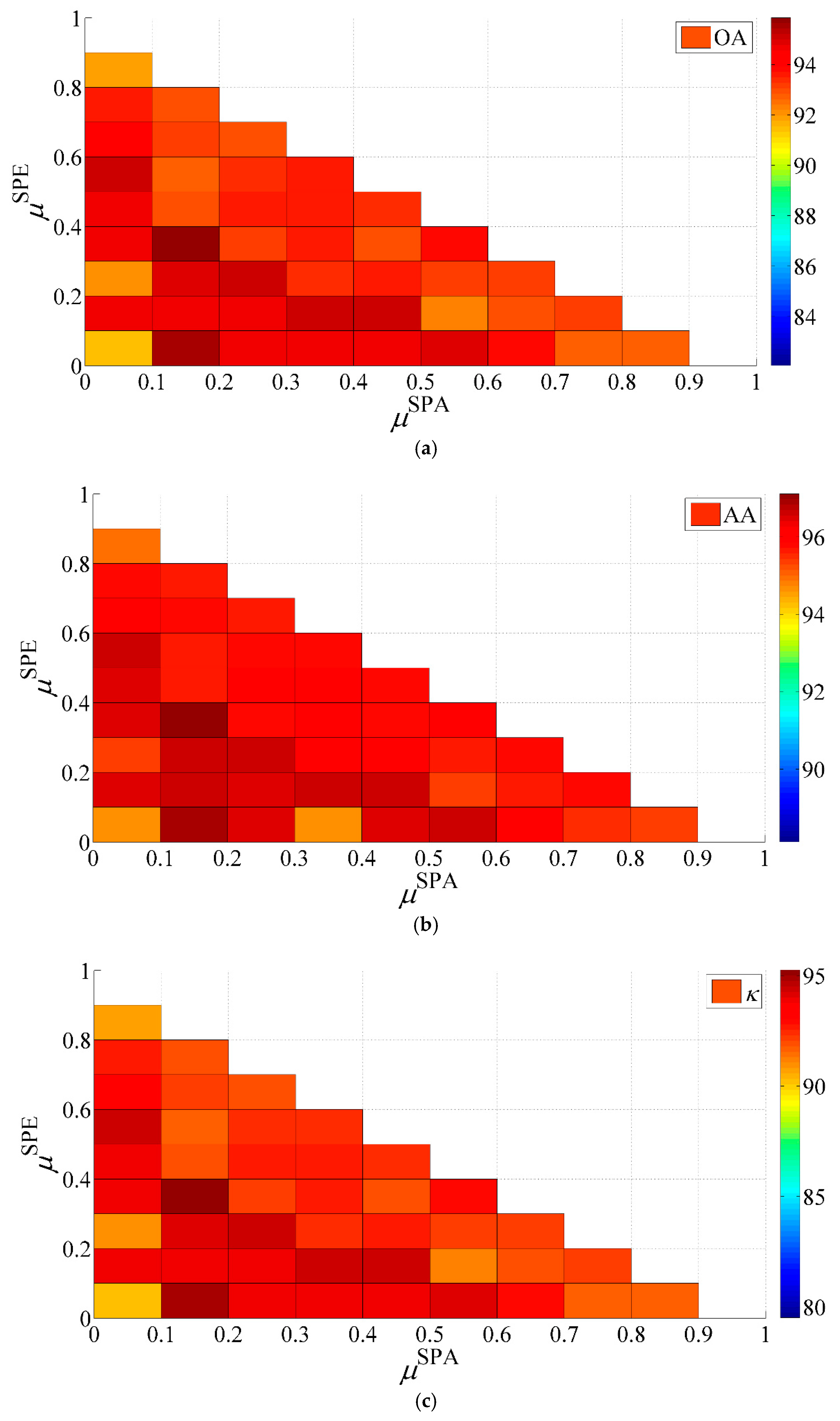
In the SVM-SSK method, the weights in $K^{\mathit{SPE}-\mathit{SPA}-\mathit{HIE}}$ critically determine the classification performance, since their values indicate the contribution of spectral, spatial, and hierarchical structure information for classification. An appropriate combination of their values may obtain better results. To obtain the interaction effect of ${\mu }^{\mathit{SPE}}$, ${\mu }^{\mathit{SPA}}$, and ${\mu }^{\mathit{HIE}}$, we can perform a four-dimensional (4-D) analysis to evaluate the influence of these three weights on our method’s performance. Based on the constraint of ${\mu }^{\mathit{SPE}}+{\mu }^{\mathit{SPA}}+{\mu }^{\mathit{HIE}}=1$, we converted this 4-D analysis to a problem of analyzing different combinations of ${\mu }^{\mathit{SPE}}$ and ${\mu }^{\mathit{SPA}}$ in terms of classification accuracies. Figure 6 illustrates the three-dimensional (3-D) plot of the classification accuracies with the change of ${\mu }^{\mathit{SPE}}$ and ${\mu }^{\mathit{SPA}}$ from 0 to 1 with a step size of 0.1. Several conclusions can be observed from this figure.

First, for the IP image, if ${\mu }^{\mathit{SPE}}=0$, it means that the proposed framework includes only two kernels of $K^{\mathit{SPA}}$ and $K^{\mathit{HIE}}$. In such case, we can obtain the OA, AA and κ with 91.01%~95.59%, 93.53%~96.91%, and 89.69%~94.95%, respectively; if ${\mu }^{\mathit{SPA}}=0$, it indicates that the proposed framework includes only two kernels of $K^{\mathit{SPE}}$ and $K^{\mathit{HIE}}$. In such a case, we can obtain the OA, AA and κ with 82.06%~95.1%, 88.12%~96.65%, and 79.51%~94.38%, respectively. Specifically, the OA, AA and κ of 91.52%, 94.7%, and 90.31% were achieved when ${\mu }^{\mathit{SPE}}={\mu }^{\mathit{SPA}}=0$. For the UP image, the OA, AA, and κ can be obtained with 61.28%~98.05%, 70.91%~98.68%, and 52.53%~97.42% when ${\mu }^{\mathit{SPE}}=0$, respectively, and 61.28%~92.86%, 70.91%~95.27%, and 52.53%~90.65% when ${\mu }^{\mathit{SPA}}=0$, respectively. Specifically, the very poor OA, AA, and κ of 61.28%, 70.91%, and 52.53% were achieved when ${\mu }^{\mathit{SPE}}={\mu }^{\mathit{SPA}}=0$, respectively.

Second, the appropriate selection of ${\mu }^{\mathit{SPE}}$, ${\mu }^{\mathit{SPA}}$, and ${\mu }^{\mathit{HIE}}$ can result in the best classification accuracies. For instance, the highest OA, AA, and κ for the IP and UP images can reach to 95.86%, 97.12%, and 95.25% under the condition of ${\mu }^{\mathit{SPE}}=0.3$, ${\mu }^{\mathit{SPA}}=0.1$, and ${\mu }^{HIE}=0.6$, and to 98.14%, 98.75%, and 97.53% under the condition of ${\mu }^{\mathit{SPE}}=0.1$, ${\mu }^{\mathit{SPA}}=0.7$, and ${\mu }^{HIE}=0.2$, respectively. Compared to Table 2 and Table 4, it can be confirmed again that the combination of the spectral, spatial and hierarchical kernels is really essential to produce better classification accuracies than using a single or double kernels in the SVM classifier.

Finally, the SVM-SSHK method can demonstrate very stable classification performance in most cases of different parameter settings on ${\mu }^{\mathit{SPE}}$ and ${\mu }^{\mathit{SPA}}$. According to Figure 6, there are 66 combinations of the two weights in total. For the IP image, the SVM-SSHK method can obtain the OA, AA and κ higher than 92%, 94%, and 90% for 53 of 66 (80.30%) different parameters settings, respectively. For the UP image, the proposed method is capable of achieving the OA, AA, and κ higher than 95%, 95%, and 90% for 40 of 66 (60.60%) different parameters settings, respectively.

6. Conclusions

In this paper, we present an effective classification framework by integrating the spectral, spatial, and hierarchical structure information into the SVM classifier in a way of multiple kernels. In this framework, the spectral kernel is constructed using directly the original HSI, the spatial kernel is modeled using the EMP method and the hierarchical kernel is introduced by combining the techniques of FMS and AMG-MHSEG. The main advantage of the proposed framework is to utilize spatial structure information in multiple scales for HSI classification. Experimental results on two benchmark HSIs confirmed the following conclusions: (1) The combination of the spectral, spatial and hierarchical kernels in the SVM-SSHK method can generate better classification results than using any single or double of these three kernels; (2) The SVM-SSHK method can achieve the most accurate classification results under different training sets, when compared to the popular kernel-based classification methods. Specifically, SVM-SSHK can be 0.02–15.24% and 0.08–15.61% higher than the other methods in average in the terms of OA for the IP and UP images, respectively; (3) SVM-SSHK can demonstrate stable classification performance in most cases of different parameter settings on the weights of the three kernels. In conclusion, the SVM-SSHK method is very promising for the improvement of classification of hyperspectral images. In the future, advanced studies will be performed by exploring more efficient SVMs with multiple kernels.

References

- Cloutis, E.A. Review article hyperspectral geological remote sensing: Evaluation of analytical techniques. Int. J. Remote Sens. 1996, 17, 2215–2242. [Google Scholar] [CrossRef]
- Kruse, F.A.; Boardman, J.W.; Huntington, J.F. Comparison of airborne hyperspectral data and eo-1 hyperion for mineral mapping. IEEE Trans. Geosci. Remote Sens. 2003, 41, 1388–1400. [Google Scholar] [CrossRef]
- Cochrane, M.A. Using vegetation reflectance variability for species level classification of hyperspectral data. Int. J. Remote Sens. 2000, 21, 2075–2087. [Google Scholar] [CrossRef]
- Strachan, I.B.; Pattey, E.; Boisvert, J.B. Impact of nitrogen and environmental conditions on corn as detected by hyperspectral reflectance. Remote Sens. Environ. 2002, 80, 213–224. [Google Scholar] [CrossRef]
- Dahan, M. Compressive fluorescence microscopy for biological and hyperspectral imaging. Proceed. Natl. Acad. Sci. USA 2012, 109, 1679–1687. [Google Scholar]
- Hughes, G. On the mean accuracy of statistical pattern recognizers. Inf. Theory IEEE Trans. 1968, 14, 55–63. [Google Scholar] [CrossRef]
- Fauvel, M.; Tarabalka, Y.; Benediktsson, J.A.; Chanussot, J.; Tilton, J.C. Advances in spectral-spatial classification of hyperspectral images. Proc. IEEE 2013, 101, 652–675. [Google Scholar] [CrossRef]
- Camps-Valls, G.; Tuia, D.; Bruzzone, L.; Benediktsson, J.A. Advances in hyperspectral image classification: Earth monitoring with statistical learning methods. IEEE Signal Process. Mag. 2014, 31, 45–54. [Google Scholar] [CrossRef]
- Yang, H. A back-propagation neural network for mineralogical mapping from aviris data. Int. J. Remote Sens. 1999, 20, 97–110. [Google Scholar] [CrossRef]
- Melgani, F.; Bruzzone, L. Classification of hyperspectral remote sensing images with support vector machines. IEEE Trans. Geosci. Remote Sens. 2004, 42, 1778–1790. [Google Scholar] [CrossRef]
- Ham, J.; Chen, Y.; Crawford, M.M.; Ghosh, J. Investigation of the random forest framework for classification of hyperspectral data. IEEE Trans. Geosci. Remote Sens. 2005, 43, 492–501. [Google Scholar] [CrossRef]
- Chen, C.H.; Peter Ho, P.-G. Statistical pattern recognition in remote sensing. Pattern Recognit. 2008, 41, 2731–2741. [Google Scholar] [CrossRef]
- Camps-Valls, G.; Bruzzone, L. Kernel Methods for Remote Sensing Data Analysis; Wiley: New York, NY, USA, 2009. [Google Scholar]
- Ratle, F.; Camps-Valls, G.; Weston, J. Semisupervised neural networks for efficient hyperspectral image classification. IEEE Trans. Geosci. Remote Sens. 2010, 48, 2271–2282. [Google Scholar] [CrossRef]
- Cortes, C.; Vapnik, V. Support vector machine. Mach. Learn. 1995, 20, 273–297. [Google Scholar] [CrossRef]
- Böhning, D. Multinomial logistic regression algorithm. Ann. Inst. Stat. Math. 1992, 44, 197–200. [Google Scholar] [CrossRef]
- Li, J.; Bioucas-Dias, J.M.; Plaza, A. Semisupervised hyperspectral image segmentation using multinomial logistic regression with active learning. IEEE Trans. Geosci. Remote Sens. 2010, 48, 4085–4098. [Google Scholar] [CrossRef]
- Li, J.; Bioucas-Dias, J.M.; Plaza, A. Spectral-spatial hyperspectral image segmentation using subspace multinomial logistic regression and markov random fields. IEEE Trans. Geosci. Remote Sens. 2012, 50, 809–823. [Google Scholar] [CrossRef]
- Plaza, A.; Benediktsson, J.A.; Boardman, J.W.; Brazile, J.; Bruzzone, L.; Camps-Valls, G.; Chanussot, J.; Fauvel, M.; Gamba, P.; Gualtieri, A. Recent advances in techniques for hyperspectral image processing. Remote Sens. Environ. 2009, 113, S110–S122. [Google Scholar] [CrossRef]
- Camps-Valls, G.; Gomez-Chova, L.; Munoz-Mari, J.; Vila-Frances, J.; Calpe-Maravilla, J. Composite kernels for hyperspectral image classification. IEEE Geosci. Remote Sens. Lett. 2006, 3, 93–97. [Google Scholar] [CrossRef]
- Camps-Valls, G.; Shervashidze, N.; Borgwardt, K.M. Spatio-spectral remote sensing image classification with graph kernels. IEEE Geosci. Remote Sens. Lett. 2010, 7, 741–745. [Google Scholar] [CrossRef]
- Mathieu, F.; Jocelyn, C.; Atli, B.J. A spatial-spectral kernel-based approach for the classification of remote-sensing images. Pattern Recognit. 2012, 45, 381–392. [Google Scholar]
- Wang, Y.; Zhang, Y.; Song, H. A spectral-texture kernel-based classification method for hyperspectral images. Remote Sens. 2016, 8, 919. [Google Scholar] [CrossRef]
- Fauvel, M.; Chanussot, J.; Benediktsson, J.A. A spatial-spectral kernel-based approach for the classification of remote-sensing images. Pattern Recognit. 2012, 45, 381–392. [Google Scholar] [CrossRef]
- Shen, L.; Zhu, Z.; Jia, S.; Zhu, J.; Sun, Y. Discriminative gabor feature selection for hyperspectral image classification. IEEE Geosci. Remote Sens. Lett. 2013, 10, 29–33. [Google Scholar] [CrossRef]
- Huang, X.; Zhang, L. A comparative study of spatial approaches for urban mapping using hyperspectral rosis images over pavia city, northern italy. Int. J. Remote Sens. 2009, 30, 3205–3221. [Google Scholar] [CrossRef]
- Kang, X.; Li, S.; Benediktsson, J.A. Spectral-spatial hyperspectral image classification with edge-preserving filtering. IEEE Trans. Geosci. Remote Sens. 2014, 52, 2666–2677. [Google Scholar] [CrossRef]
- Benediktsson, J.A.; Palmason, J.A.; Sveinsson, J.R. Classification of hyperspectral data from urban areas based on extended morphological profiles. IEEE Trans. Geosci. Remote Sens. 2005, 43, 480–491. [Google Scholar] [CrossRef]
- Huang, X.; Zhang, L. An adaptive mean-shift analysis approach for object extraction and classification from urban hyperspectral imagery. IEEE Trans. Geosci. Remote Sens. 2008, 46, 4173–4185. [Google Scholar] [CrossRef]
- Tarabalka, Y.; Chanussot, J.; Benediktsson, J.A. Segmentation and classification of hyperspectral images using watershed transformation. Pattern Recognit. 2010, 43, 2367–2379. [Google Scholar] [CrossRef]
- Tarabalka, Y.; Tilton, J.C.; Benediktsson, J.A.; Chanussot, J. A marker-based approach for the automated selection of a single segmentation from a hierarchical set of image segmentations. IEEE J. Sel. Top. Appl. Earth Obs. Remote Sens. 2012, 5, 262–272. [Google Scholar] [CrossRef]
- Song, H.; Wang, Y. A spectral-spatial classification of hyperspectral images based on the algebraic multigrid method and hierarchical segmentation algorithm. Remote Sens. 2016, 8, 296. [Google Scholar] [CrossRef]
- Tarabalka, Y.; Chanussot, J.; Benediktsson, J.A. Segmentation and classification of hyperspectral images using minimum spanning forest grown from automatically selected markers. IEEE Trans. Syst. Man Cybern. 2010, 40, 1267–1279. [Google Scholar] [CrossRef] [PubMed]
- Tarabalka, Y.; Rana, A. Graph-Cut-Based Model for Spectral-Spatial Classification of Hyperspectral Images. In Proceedings of the IEEE Geoscience and Remote Sensing Symposium, Quebec City, QC, Canada, 13–18 July 2014; pp. 3418–3421. [Google Scholar]
- Wang, Y.; Song, H.; Zhang, Y. Spectral-spatial classification of hyperspectral images using joint bilateral filter and graph cut based model. Remote Sens. 2016, 8, 748. [Google Scholar] [CrossRef]
- Fang, L.; Li, S.; Kang, X.; Benediktsson, J.A. Spectral-spatial classification of hyperspectral images with a superpixel-based discriminative sparse model. IEEE Trans. Geosci. Remote Sens. 2015, 53, 4186–4201. [Google Scholar] [CrossRef]
- Farag, A.A.; Mohamed, R.M.; El-Baz, A. A unified framework for map estimation in remote sensing image segmentation. IEEE Trans. Geosci. Remote Sens. 2005, 43, 1617–1634. [Google Scholar] [CrossRef]
- Tarabalka, Y.; Fauvel, M.; Chanussot, J.; Benediktsson, J.A. Svm-and mrf-based method for accurate classification of hyperspectral images. IEEE Geosci. Remote Sens. Lett. 2010, 7, 736–740. [Google Scholar] [CrossRef]
- Zhang, B.; Li, S.; Jia, X.; Gao, L.; Peng, M. Adaptive markov random field approach for classification of hyperspectral imagery. IEEE Geosci. Remote Sens. Lett. 2011, 8, 973–977. [Google Scholar] [CrossRef]
- Moser, G.; Serpico, S.B. Combining support vector machines and markov random fields in an integrated framework for contextual image classification. IEEE Trans. Geosci. Remote Sens. 2013, 51, 2734–2752. [Google Scholar] [CrossRef]
- Bai, J.; Xiang, S.; Pan, C. A graph-based classification method for hyperspectral images. IEEE Trans. Geosci. Remote Sens. 2013, 51, 803–817. [Google Scholar] [CrossRef]
- Ghamisi, P.; Benediktsson, J.A.; Ulfarsson, M.O. Spectral-spatial classification of hyperspectral images based on hidden markov random fields. IEEE Trans. Geosci. Remote Sens. 2014, 52, 2565–2574. [Google Scholar] [CrossRef]
- Golipour, M.; Ghassemian, H.; Mirzapour, F. Integrating hierarchical segmentation maps with mrf prior for classification of hyperspectral images in a bayesian framework. IEEE Trans. Geosci. Remote Sens. 2016, 54, 805–816. [Google Scholar] [CrossRef]
- Fauvel, M.; Benediktsson, J.A.; Chanussot, J.; Sveinsson, J.R. Spectral and spatial classification of hyperspectral data using svms and morphological profiles. IEEE Trans. Geosci. Remote Sens. 2008, 46, 3804–3814. [Google Scholar] [CrossRef]
- Li, J.; Marpu, P.R.; Plaza, A.; Bioucas-Dias, J.M.; Benediktsson, J.A. Generalized composite kernel framework for hyperspectral image classification. IEEE Trans. Geosci. Remote Sens. 2013, 51, 4816–4829. [Google Scholar] [CrossRef]
- Fang, L.; Li, S.; Duan, W.; Ren, J.; Benediktsson, J.A. Classification of hyperspectral images by exploiting spectral-spatial information of superpixel via multiple kernels. IEEE Trans. Geosci. Remote Sens. 2015, 53, 6663–6674. [Google Scholar] [CrossRef]
- Lu, T.; Li, S.; Fang, L.; Jia, X.; Benediktsson, J.A. From subpixel to superpixel: A novel fusion framework for hyperspectral image classification. IEEE Trans. Geosci. Remote Sens. 2017, 55, 4398–4411. [Google Scholar] [CrossRef]
- Peng, J.; Chen, H.; Zhou, Y.; Li, L. Ideal regularized composite kernel for hyperspectral image classification. IEEE J. Sel. Top. Appl. Earth Obs. Remote Sens. 2017, 10, 1563–1574. [Google Scholar] [CrossRef]
- Palmason, J.A.; Benediktsson, J.A.; Sveinsson, J.R.; Chanussot, J. Classification of Hyperspectral Data from Urban Areas Using Morphological Preprocessing and Independent Component Analysis. In Proceedings of the 2005 IEEE International Geoscience and Remote Sensing Symposium, Seoul, Korea, 25–29 July 2005; p. 4. [Google Scholar]
- Fauvel, M.; Chanussot, J.; Benediktsson, J.A. Kernel principal component analysis for the classification of hyperspectral remote sensing data over urban areas. EURASIP J. Adv. Signal Process. 2009, 2009, 783194. [Google Scholar] [CrossRef]
- Castaings, T.; Waske, B.; Atli Benediktsson, J.; Chanussot, J. On the influence of feature reduction for the classification of hyperspectral images based on the extended morphological profile. Int. J. Remote Sens. 2010, 31, 5921–5939. [Google Scholar] [CrossRef]
- Pal, M.; Foody, G.M. Feature selection for classification of hyperspectral data by svm. IEEE Trans. Geosci. Remote Sens. 2010, 48, 2297–2307. [Google Scholar] [CrossRef]
- Tuia, D.; Camps-Valls, G.; Matasci, G.; Kanevski, M. Learning relevant image features with multiple-kernel classification. IEEE Trans. Geosci. Remote Sens. 2010, 48, 3780–3791. [Google Scholar] [CrossRef]
- Jia, X.; Kuo, B.C.; Crawford, M.M. Feature mining for hyperspectral image classification. Proc. IEEE 2013, 101, 676–697. [Google Scholar] [CrossRef]
- Taşkın, G.; Kaya, H.; Bruzzone, L. Feature selection based on high dimensional model representation for hyperspectral images. IEEE Trans. Image Process. 2017, 26, 2918–2928. [Google Scholar] [CrossRef] [PubMed]
- Cheng, Q.; Zhou, H.; Cheng, J. The fisher-markov selector: Fast selecting maximally separable feature subset for multiclass classification with applications to high-dimensional data. IEEE Trans. Pattern Anal. Mach. Intell. 2011, 33, 1217–1233. [Google Scholar] [CrossRef] [PubMed]
- Perona, P.; Malik, J. Scale-space and edge detection using anisotropic diffusion. IEEE Trans. Pattern Anal. Mach. Intell. 1990, 12, 629–639. [Google Scholar] [CrossRef]
- Weickert, J.; Romeny, B.M.T.H.; Viergever, M.A. Efficient and reliable schemes for nonlinear diffusion filtering. IEEE Trans. Geosci. Remote Sens. 1998, 7, 398–410. [Google Scholar] [CrossRef] [PubMed]
- Falgout, R.D. An introduction to algebraic multigrid. Comput. Sci. Eng. 2006, 8, 24–33. [Google Scholar] [CrossRef]
- Duarte-Carvajalino, J.M.; Sapiro, G.; Vélez-Reyes, M.; Castillo, P.E. Multiscale representation and segmentation of hyperspectral imagery using geometric partial differential equations and algebraic multigrid methods. IEEE Trans. Geosci. Remote Sens. 2008, 46, 2418–2434. [Google Scholar] [CrossRef]
- Briggs, W.L.; Henson, V.E.; McCormick, S.F. A Multigrid Tutorial, 2nd ed.; SIAM: Philadelphia, PA, USA, 2000; pp. 7–48. [Google Scholar]
- Cristianini, N.; Scholkopf, B. Support vector machines and kernel methods: The new generation of learning machines. Ai Mag. 2002, 23, 31. [Google Scholar]
- Schölkopf, B.; Smola, A.J. Learning with Kernels. Support Vector Machines, Regularization, Optimization, and Beyond; MIT Press: Cambridge, MA, USA, 2002. [Google Scholar]
Figure 1.
The multigrid structure of hyperspectral images (HSIs).
Figure 2.
Schematic diagram of the SVM-SSHK method.
Figure 3.
Hyperspectral images and the corresponding ground truth data (GTD). (a) A false color composite image (bands 47, 23, and 13) of the Indian Pines (IP) image and (b) its GTD; (c) a false color composite image (bands 103, 56, and 31) of the University of Pavia (UP) image and (d) its GTD.
Figure 4.
Classification results of the IP image. (a) SVM; (b) EMP; (c) EPF; (d) SVM-CK; (e) MLR-GCK; (f) SC-SSK; (g) SC-MK; and, (h) SVM-SSHK.
Figure 5.
Classification results of the UP image. (a) SVM; (b) EMP; (c) EPF; (d) SVM-CK; (e) MLR-GCK; (f) SC-SSK; (g) SC-MK; and, (h) SVM-SSHK.
Figure 6.
Impact of and using the two images on SVM-SSHK’s performance. (a) overall accuracy (OA); (b) average accuracy (AA); and, (c) kappa coefficient (κ) for the IP image; (d) OA; (e) AA and (f) κ for the UP image.