Development of a Regional Lidar-Derived Above-Ground Biomass Model with Bayesian Model Averaging for Use in Ponderosa Pine and Mixed Conifer Forests in Arizona and New Mexico, USA

 ,
,
Abstract
:
1. Introduction
1.1. Background
1.2. Project Goals
2. Materials and Methods
2.1. Study Area
2.2. Data
2.2.1. Field Survey
2.2.2. Lidar
2.2.3. Topography
2.2.4. Phenology
2.2.5. Ecological Response Unit
2.3. Field AGB Estimates
2.4. Estimating AGB with Lidar Metrics and Ancillary Data
2.4.1. Variable Selection with Bayesian Model Averaging and Stepwise Regression
2.4.2. BMA Specifications
2.5. Model Evaluation and Assessment of Lidar AGB Estimates
2.5.1. Comparison of Product from Four Model Selection Procedures
2.5.2. Model Refinement to Reduce Variance Inflation and Increase Reliability of Model Coefficients
2.5.3. Model Performance by Project and Plot Size
3. Results
3.1. Summary Statistics of Field Data Estimates
3.2. Assessing Results of Alternative Variable Selection Procedures
3.3. Median Probability AGB Model Structure
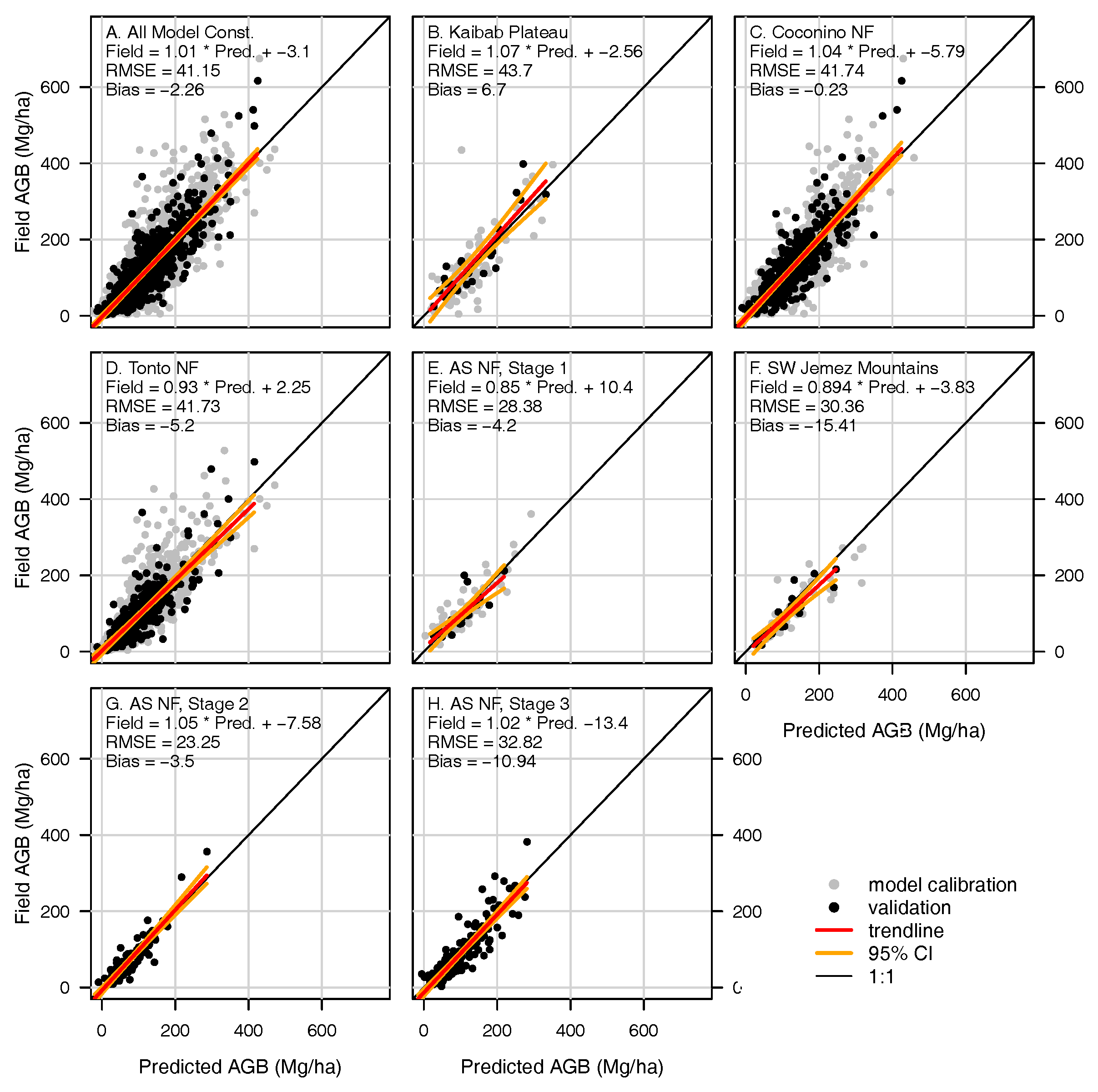
3.4. Trimmed Median Probability Model Performance, Overall and by Field Data Collection Site
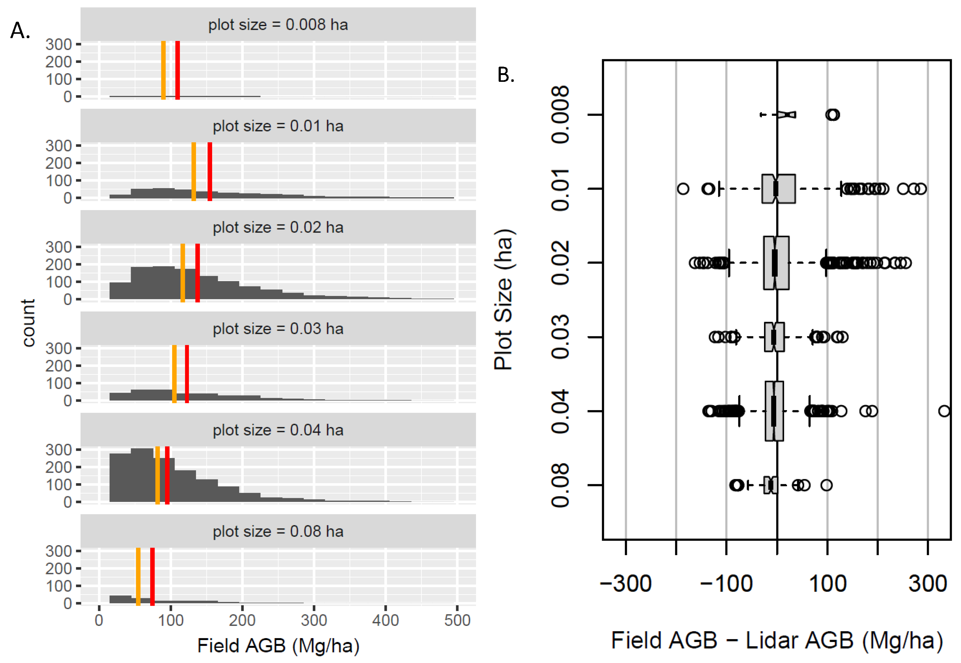
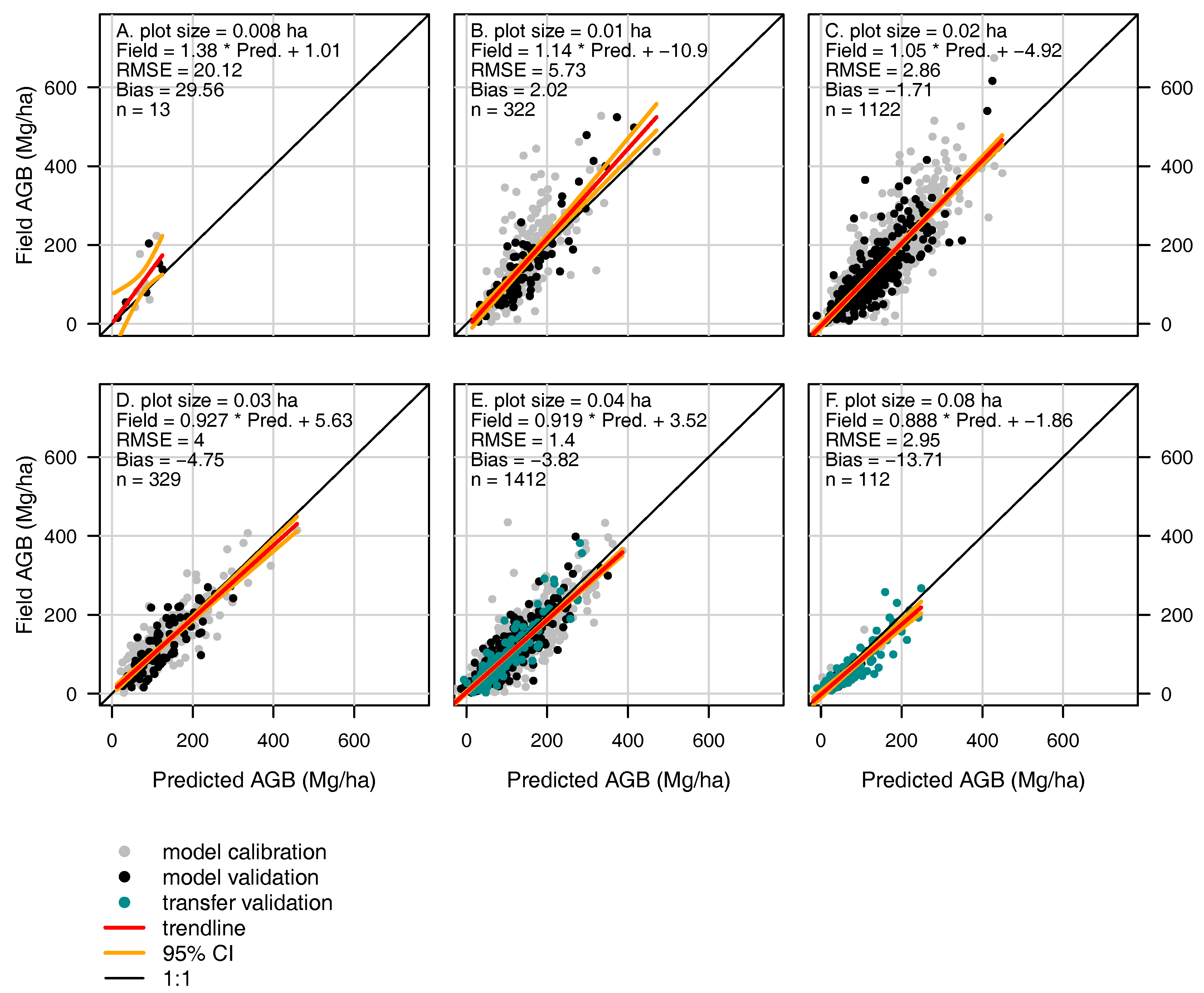
3.5. Influence of Inconsistent Plot Size
4. Discussion
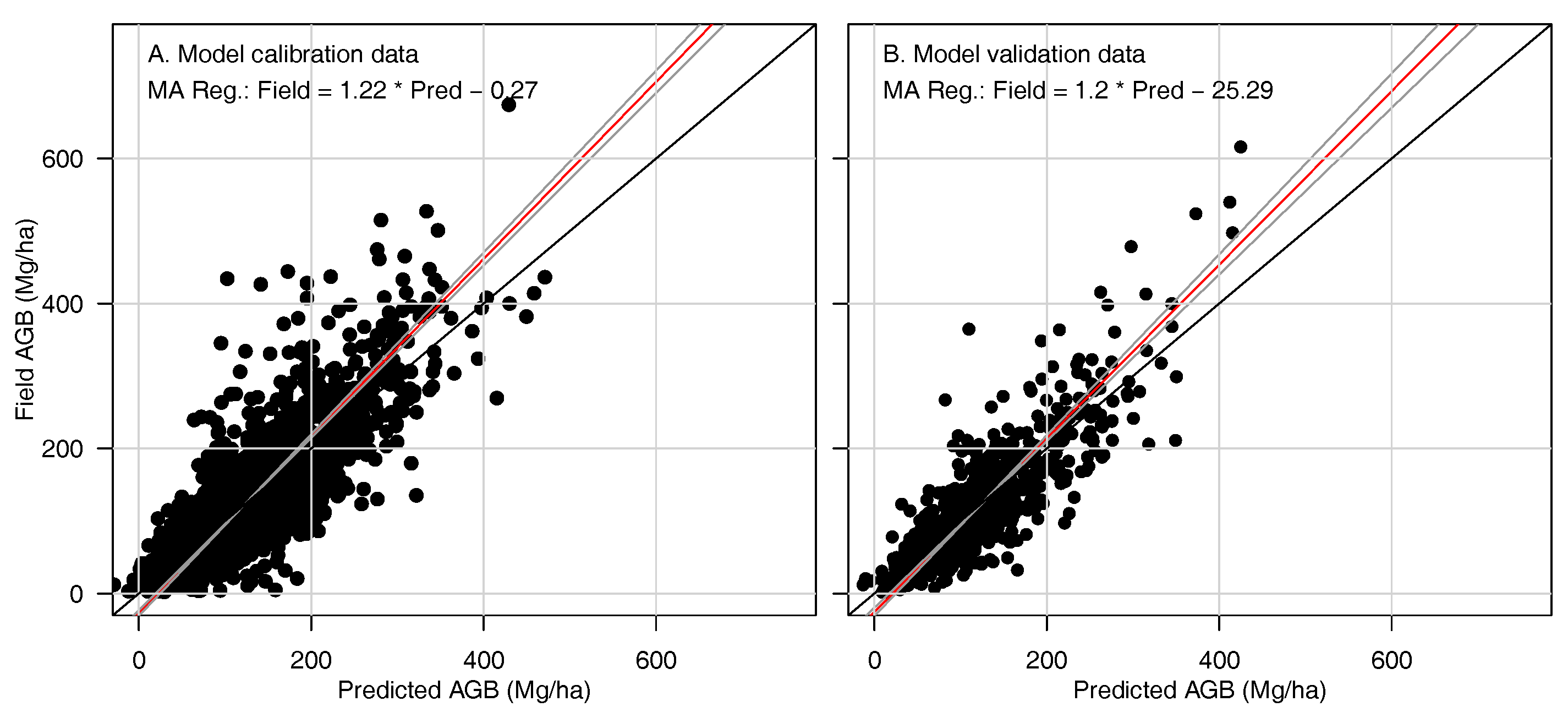
4.1. Model Bias
4.2. Relationship to Other Modeling Efforts
4.3. Management Implications
5. Conclusions
Directions for Future Research
Supplementary Materials
Acknowledgments
Author Contributions
Conflicts of Interest
Abbreviations
| BMA | Bayesian model average |
| CFLRP | Collaborative Forest Landscape Restoration Program |
| dbh | diameter at breast height |
| 4FRI | Four Forest Restoration Initiative |
| N.F. | National Forest |
| PRSE | percent relative standard error |
| RMSE | root mean square error |
| RMSPE | root mean square predicted error |
References
- Brown, R.T.; Agee, J.K.; Franklin, J.F. Forest restoration and fire: Principles in the context of place. Conserv. Biol. 2004, 18, 903–912. [Google Scholar] [CrossRef]
- Jolly, W.M.; Cochrane, M.A.; Freeborn, P.H.; Holden, Z.A.; Brown, T.J.; Williamson, G.J.; Bowman, D.M. Climate-induced variations in global wildfire danger from 1979 to 2013. Nat. Commun. 2015, 6, 7537. [Google Scholar] [CrossRef] [PubMed]
- Covington, W.W.; Moore, M.M. Post settlement changes in natural fire regimes and forest structure: Ecological restoration of old-growth ponderosa pine forests. J. Sustain. For. 1994, 2, 153–181. [Google Scholar] [CrossRef]
- Huffman, D.W.; Zegler, T.J.; Fule, P.Z. Fire history of a mixed conifer forest on the Mogollon Rim, northern Arizona, USA. Int. J. Wildland Fire 2015, 24, 680–689. [Google Scholar] [CrossRef]
- Cooper, E. Changes in vegetation, structure, and growth of southwestern pine forest since white settlement. Ecol. Mon. 1960, 30, 129–164. [Google Scholar] [CrossRef]
- Moore, M.M.; Huffman, D.W.; Fule, P.Z.; Covington, W.W.; Crouse, J.E. Comparison of historical and contemporary forest structure and composition on permanent plots in southwestern ponderosa pine forest. For. Sci. 2004, 50, 162–176. [Google Scholar]
- Strahan, R.T.; Sánchez Meador, A.J.; Huffman, D.W.; Laughlin, D.C. Shifts in community-level traits and functional diversity in a mixed conifer forest: A legacy of land-use change. J. Appl. Ecol. 2016, 53, 1755–1765. [Google Scholar] [CrossRef]
- Flannigan, M.D.; Stocks, B.J.; Wotton, B.M. Climate change and forest fires. Sci. Total Environ. 2000, 262, 221–229. [Google Scholar] [CrossRef]
- McKenzie, D.; Gedalof, Z.E.; Peterson, D.L.; Mote, P. Climatic change, wildfire, and conservation. Conserv. Biol. 2004, 18, 890–902. [Google Scholar]
- Westerling, A.L.; Hidalgo, H.G.; Cayan, D.R.; Swetnam, T.W. Warming and earlier spring increase western US forest wildfire activity. Science 2006, 313, 940–943. [Google Scholar] [CrossRef] [PubMed]
- Liu, Y.; Stanturf, J.; Goodrick, S. Trends in global wildfire potential in a changing climate. For. Ecol. Manag. 2010, 259, 685–697. [Google Scholar] [CrossRef]
- Seidl, R.; Thom, D.; Kautz, M.; Martin-Benito, D.; Peltoniemi, M.; Vacchiano, G.; Wild, J.; Ascoli, D.; Petr, M.; Honkaniemi, J.; et al. Forest disturbances under climate change. Nat. Clim. Chang. 2017, 7, 395–402. [Google Scholar] [CrossRef] [PubMed]
- Abatzoglou, J.T.; Williams, A.P. Impact of anthropogenic climate change on wildfire across western US forests. Proc. Natl. Acad. Sci. USA 2016, 113, 11770–11775. [Google Scholar] [CrossRef] [PubMed]
- Schultz, C.A.; Jedd, T.; Beam, R.D. The Collaborative Forest Landscape Restoration Program: A history and overview of the first projects. J. For. 2012, 110, 381–391. [Google Scholar] [CrossRef]
- Schoennagel, T.; Nelson, C.R.; Theobald, D.M.; Carnwath, G.C.; Chapman, T.B. Implementation of National Fire Plan treatments near the wildland–urban interface in the western United States. Proc. Natl. Acad. Sci. USA 2009, 106, 10706–10711. [Google Scholar] [CrossRef] [PubMed]
- Nagendra, H.; Lucas, R.; Honrado, J.P.; Jongman, R.H.; Tarantino, C.; Adamo, M.; Mairota, P. Remote sensing for conservation monitoring: Assessing protected areas, habitat extent, habitat condition, species diversity, and threats. Ecol. Indic. 2013, 33, 45–59. [Google Scholar] [CrossRef]
- Dubayah, R.; Drake, J.B. Lidar remote sensing for forestry. J. For. 2000, 98, 44–46. [Google Scholar]
- Lefsky, M.A.; Cohen, W.B.; Parker, G.G.; Harding, D.J. Lidar remote sensing for ecosystem studies: Lidar, an emerging remote sensing technology that directly measures the three-dimensional distribution of plant canopies, can accurately estimate vegetation structural attributes and should be of particular interest to forest, landscape, and global ecologists. AIBS Bull. 2002, 52, 19–30. [Google Scholar]
- Hyyppä, J.; Hyyppä, H.; Leckie, D.; Gougeon, F.; Yu, X.; Maltamo, M. Review of methods of small-footprint airborne laser scanning for extracting forest inventory data in boreal forests. Int. J. Remote Sens. 2008, 29, 1339–1366. [Google Scholar] [CrossRef]
- Goetz, S.J.; Dubayah, R.O. Advances in remote sensing technology and implications for measuring and monitoring forest carbon stocks and change. Carbon Manag. 2011, 2, 231–244. [Google Scholar] [CrossRef]
- Petrokofsky, G.; Kanamaru, H.; Achard, F.; Goetz, S.J.; Joosten, H.; Holmgren, P.; Lehtonen, A.; Menton, M.C.S.; Pullin, A.S.; Wattenbach, M. Comparison of methods for measuring and assessing carbon stocks and carbon stock changes in terrestrial carbon pools. How do the accuracy and precision of current methods compare? A systematic review protocol. Environ. Evid. 2012, 1, 6. [Google Scholar] [CrossRef] [Green Version]
- Wulder, M.A.; White, J.C.; Nelson, R.F.; Næsset, E.; Ørka, H.O.; Coops, N.C.; Hilker, T.; Bater, C.W.; Gobakken, T. Lidar sampling for large-area forest characterization: A review. Remote Sens. Environ. 2012, 121, 196–209. [Google Scholar] [CrossRef]
- Zolkos, S.G.; Goetz, S.J.; Dubayah, R. A meta-analysis of terrestrial aboveground biomass estimation using lidar remote sensing. Remote Sens. Environ. 2013, 128, 289–298. [Google Scholar] [CrossRef]
- Reinhardt, E.D.; Keane, R.E.; Calkin, D.E.; Cohen, J.D. Objectives and considerations for wildland fuel treatment in forested ecosystems of the interior western United States. For. Ecol. Manag. 2008, 256, 1997–2006. [Google Scholar] [CrossRef]
- Gaines, W.L.; Harrod, R.J.; Dickinson, J.; Lyons, A.L.; Halupka, K. Integration of Northern spotted owl habitat and fuels treatments in the eastern Cascades, Washington, USA. For. Ecol. Manag. 2010, 260, 2045–2052. [Google Scholar] [CrossRef]
- Roccaforte, J.P.; Fule, P.Z.; Covington, W.W. Monitoring Landscape-Scale Ponderosa Pine Restoration Treatment Implementation and Effectiveness. Restor. Ecol. 2010, 18, 820–833. [Google Scholar] [CrossRef]
- Schoennagel, T.; Nelson, C.R. Restoration relevance of recent National Fire Plan treatments in forests of the western United States. Front. Ecol. Environ. 2010, 9, 271–277. [Google Scholar] [CrossRef]
- Schultz, C.A.; Coelho, D.L.; Beam, R.D. Design and governance of multiparty monitoring under the USDA Forest Service’s Collaborative Forest Landscape Restoration Program. J. For. 2014, 112, 198–206. [Google Scholar] [CrossRef]
- Ringold, P.L.; Alegria, J.; Czaplewski, R.L.; Mulder, B.S.; Tolle, T.; Burnett, K. Adaptive monitoring design for ecosystem management. Ecol. Appl. 1996, 6, 745–747. [Google Scholar] [CrossRef]
- Stankey, G.H.; Bormann, B.T.; Ryan, C.; Shindler, B.; Sturtevant, V.; Clark, R.N.; Philpot, C. Adaptive management and the Northwest Forest Plan: Rhetoric and reality. J. For. 2003, 101, 40–46. [Google Scholar]
- Stem, C.; Margoluis, R.; Salafsky, N.; Brown, M. Monitoring and evaluation in conservation: A review of trends and approaches. Conserv. Biol. 2005, 19, 295–309. [Google Scholar] [CrossRef]
- Larson, A.J.; Belote, R.T.; Williamson, M.A.; Aplet, G.H. Making monitoring count: Project design for active adaptive management. J. For. 2013, 111, 348–356. [Google Scholar] [CrossRef]
- Folke, C.; Carpenter, S.; Elmqvist, T.; Gunderson, L.; Holling, C.S.; Walker, B. Resilience and sustainable development: Building adaptive capacity in a world of transformations. AMBIO J. Hum. Environ. 2002, 31, 437–440. [Google Scholar] [CrossRef]
- Hobbs, R.J.; Arico, S.; Aronson, J.; Baron, J.S.; Bridgewater, P.; Cramer, V.A.; Epstein, P.R.; Ewel, J.J.; Klink, C.S.; Lugo, A.E.; et al. Novel ecosystems: Theoretical and management aspects of the new ecological world order. Glob. Ecol. Biogeogr. 2006, 15, 1–7. [Google Scholar] [CrossRef]
- Hobbs, R.J.; Higgs, E.; Harris, J.A. Novel ecosystems: Implications for conservation and restoration. Trends Ecol. Evol. 2009, 24, 599–605. [Google Scholar] [CrossRef] [PubMed]
- Roccaforte, J.P.; Huffman, D.W.; Fulé, P.Z.; Covington, W.W.; Chancellor, W.W.; Stoddard, M.T.; Crouse, J.E. Forest structure and fuels dynamics following ponderosa pine restoration treatments, White Mountains, Arizona, USA. For. Ecol. Manag. 2015, 337, 174–185. [Google Scholar] [CrossRef]
- Sherrill, K.R.; Lefsky, M.A.; Bradford, J.B.; Ryan, M.G. Forest structure estimation and pattern exploration from discrete-return lidar in subalpine forests of the central Rockies. Can. J. For. Res. 2008, 38, 2081–2096. [Google Scholar] [CrossRef]
- Kim, Y.; Yang, Z.; Cohen, W.; Pflugmacher, D.; Lauver, C.; Vankat, J. Distinguishing between live and dead standing tree biomass on the North Rim of Grand Canyon National Park, USA using small-footprint lidar data. Remote Sens. Environ. 2009, 113, 2499–2510. [Google Scholar] [CrossRef]
- Hall, S.A.; Burke, I.C.; Box, D.O.; Kaufmann, M.R.; Stoker, J.M. Estimating stand structure using discrete-return lidar: An example from low density, fire prone ponderosa pine forests. For. Ecol. Manag. 2005, 208, 189–209. [Google Scholar] [CrossRef]
- Næsset, E. Practical large-scale forest stand inventory using small-footprint airborne scanning laser. Scand. J. For. Res. 2004, 19, 164–179. [Google Scholar] [CrossRef]
- Nelson, R.; Short, A.; Valenti, M. Measuring biomass and carbon in Delaware using an airborne profiling LIDAR. Scand. J. For. Res. 2004, 19, 500–511. [Google Scholar] [CrossRef]
- Næsset, E.; Gobakken, T. Estimation of above-and below-ground biomass across regions of the boreal forest zone using airborne laser. Remote Sens. Environ. 2008, 112, 3079–3090. [Google Scholar] [CrossRef]
- Asner, G.P.; Mascaro, J.; Muller-Landau, H.C.; Vielledent, G.; Vaudry, R.; Rasamoelina, M.; Hall, J.S.; van Breugel, M. A universal airborne LiDAR approach for tropical forest carbon mapping. Oecologia 2012, 168, 1147–1160. [Google Scholar] [CrossRef] [PubMed]
- Lefsky, M.A.; Hudak, A.T.; Cohen, W.B.; Acker, S.A. Geographic variability in lidar predictions of forest stand structure in the Pacific Northwest. Remote Sens. Environ. 2005, 95, 532–548. [Google Scholar] [CrossRef]
- Næsset, E. Predicting forest stand characteristics with airborne scanning laser using a practical two-stage procedure and field data. Remote Sens. Environ. 2002, 80, 88–99. [Google Scholar] [CrossRef]
- Li, Y.; Andersen, H.; McGaughey, R. A comparison of statistical methods for estimating forest biomass from light detection and ranging data. West. J. Appl. For. 2008, 23, 223–231. [Google Scholar]
- Sarrazin, M.J.D.; Van Aardt, J.A.N.; Asner, G.P.; McGlinchy, J.; Messinger, D.W.; Wu, J. Fusing small-footprint waveform LiDAR and hyperspectral data for canopy-level species classification and herbaceous biomass modeling in savanna ecosystems. Can. J. Remote Sens. 2012, 37, 653–665. [Google Scholar] [CrossRef]
- Ediriweera, S.; Pathirana, S.; Danaher, T.; Nichols, D. Estimating above-ground biomass by fusion of LiDAR and multispectral data in subtropical woody plant communities in topographically complex terrain in North-eastern Australia. J. For. Res. 2014, 25, 761–771. [Google Scholar] [CrossRef]
- Laurin, G.; Chen, Q.; Lindsell, J.; Coomes, D.; Del Frate, F.; Guerriero, L.; Pirotti, F.; Valentini, R. Above ground biomass estimation in an African tropical forest with lidar and hyperspectral data. ISPRS J. Photogramm. Remote Sens. 2014, 89, 49–58. [Google Scholar] [CrossRef]
- Strunk, J.; Temesgen, H.; Andersen, H.E.; Packalen, P. Prediction of forest attributes with field plots, Landsat, and a sample of lidar strips. Photogramm. Eng. Remote Sens. 2014, 80, 143–150. [Google Scholar] [CrossRef]
- Raftery, A.E. Bayesian model selection in social research. Sociol. Methodol. 1995, 25, 111–163. [Google Scholar] [CrossRef]
- Hoeting, J.A.; Madigan, D.; Raftery, A.E.; Volinsky, C.T. Bayesian model averaging: A tutorial. Stat. Sci. 1999, 4, 382–417. [Google Scholar]
- Hoeting, J.A. Methodology for Bayesian model averaging: An update. In Proceedings of the Manuscripts of Invited Paper Presentations, International Biometric Conference, Freiburg, Germany, 21–26 July 2002. [Google Scholar]
- Andersen, H.E.; McGaughey, R.J.; Reutebuch, S.E. Estimating forest canopy fuel parameters using LIDAR data. Remote Sens. Environ. 2005, 94, 441–449. [Google Scholar] [CrossRef]
- Erdody, T.L.; Moskal, L.M. Fusion of LiDAR and imagery for estimating forest canopy fuels. Remote Sens. Environ. 2010, 114, 725–737. [Google Scholar]
- Hermosilla, T.; Ruiz, L.A.; Kazakova, A.N.; Coops, N.C.; Moskal, L.M. Estimation of forest structure and canopy fuel parameters from small-footprint full-waveform LiDAR data. Int. J. Wildland Fire 2014, 23, 224–233. [Google Scholar] [CrossRef]
- González-Ferreiro, E.; Diéguez-Aranda, U.; Crecente-Campo, F.; Barreiro-Fernández, L.; Miranda, D.; Castedo-Dorado, F. Modelling canopy fuel variables for Pinus radiata D. Don in NW Spain with low-density LiDAR data. Int. J. Wildland Fire 2014, 23, 350–362. [Google Scholar] [CrossRef]
- Fahey, T.J.; Woodbury, P.B.; Battles, J.J.; Goodale, C.L.; Hamburg, S.P.; Ollinger, S.V.; Woodall, C.W. Forest carbon storage: Ecology, management, and policy. Front. Ecol. Environ. 2010, 8, 245–252. [Google Scholar] [CrossRef]
- White, M.A.; Vankat, J.L. Middle and high elevation coniferous forest communities of the north rim region of Grand Canyon National Park, Arizona, USA. Vegetatio 1993, 109, 161–174. [Google Scholar] [CrossRef]
- Nichol, A.A. The Natural Vegetation of Arizona; College of Agriculture, University of Arizona: Tucson, AZ, USA, 1937. [Google Scholar]
- Romme, W.H.; Floyd, M.L.; Hanna, D. Historical Range of Variability and Current Landscape Condition Analysis: South Central Highlands Section, Southwestern Colorado and Northwestern New Mexico; Colorado Forest Restoration Institute at Colorado State University, and Region 2 of the U.S. Forest Service: Fort Collins, CO, USA, 2009.
- Rasmussen, D.I. Biotic communities of Kaibab Plateau, Arizona. Ecol. Monogr. 1941, 11, 229–275. [Google Scholar] [CrossRef]
- Weng, C.; Jackson, S.T. Late glacial and Holocene vegetation history and paleoclimate of the Kaibab Plateau, Arizona. Palaeogeogr. Palaeoclimatol. Palaeoecol. 1999, 153, 179–201. [Google Scholar] [CrossRef]
- Wahlberg, M.M.; Triepke, F.J.; Robbie, W.A.; Strenger, S.H.; Vandendriesche, D.; Muldavin, E.H.; Malusa, J.R. Ecological Response Units of the Southwestern United States; USDA, Forest Service Forestry Report FR-R3-XX-XX; Southwestern Region, Regional Office: Albuquerque, NM, USA, 2013; p. 201.
- Frazer, G.W.; Magnussen, S.; Wulder, M.A.; Niemann, K.O. Simulated impact of sample plot size and co-registration error on the accuracy and uncertainty of LiDAR-derived estimates of forest stand biomass. Remote Sens. Environ. 2011, 115, 636–649. [Google Scholar] [CrossRef]
- Lim, K.S.; Treitz, P.M. Estimation of Above ground Forest Biomass from Airborne Discrete Return Laser Scanner Data Using Canopy-based Quantile Estimators. Scand. J. For. Res. 2004, 19, 558–570. [Google Scholar] [CrossRef]
- Nilsson, M. Estimation of tree heights and stand volume using an airborne lidar system. Remote Sens. Environ. 1996, 56, 1–7. [Google Scholar] [CrossRef]
- Hosking, J.R.M. L-Moments: Analysis and Estimation of Distributions Using Linear Combinations of Order Statistics. J. R. Stat. Soc. Ser. B 1990, 52, 105–124. [Google Scholar]
- Næsset, E. Determination of mean tree height of forest stands using airborne laser scanner data. ISPRS J. Photogramm. Remote Sens. 1997, 52, 49–56. [Google Scholar] [CrossRef]
- Nelson, R.; Oderwald, R.; Gregoire, G. Separating the ground and airborne laser sampling phases to estimate tropical forest basal area, volume, and biomass. Rem. Sens. Environ. 1997, 60, 311–326. [Google Scholar] [CrossRef]
- Hawbaker, T.; Keuler, N.; Lesak, A.; Gobakken, T.; Contrucci, K.; Radeloff, V. Improved estimates of forest vegetation structure and biomass with a LiDAR-optimized sampling design. J. Geophys. Res. Biogeosci. 2009, 114. [Google Scholar] [CrossRef]
- Junttila, V.; Finley, A.O.; Bradford, J.B.; Kauranne, T. Strategies for minimizing sample size for use in airborne LiDAR-based forest inventory. For. Ecol. Manag. 2013, 292, 75–85. [Google Scholar] [CrossRef]
- Dyess, J.; Youtz, J.; Nicolet, T. Vegetation Monitoring and Sampling Protocols in Brief; US Department of Agriculture, Forest Service, Region 3: Albuquerque, NM, USA, 2011.
- McGaughey, R.J. FUSION/LDV: Software for LIDAR Data Analysis and Visualization, Version 3.60+; US Department of Agriculture, Forest Service, Pacific Northwest Research Station: Seattle, WA, USA, 2016; p. 123.
- Clyde, M.A.; Ghosh, J.; Littman, M.L. Bayesian adaptive sampling for variable selection and model averaging. J. Comput. Graph. Stat. 2011, 20, 80–101. [Google Scholar] [CrossRef]
- Farr, T.G.; Rosen, P.A.; Caro, E.; Crippen, R.; Duren, R.; Hensley, S.; Kobrick, M.; Paller, M.; Rodriguez, E.; Roth, L.; et al. The Shuttle Radar Topography Mission. Rev. Geophys. 2007, 45, 2. [Google Scholar] [CrossRef]
- Gorelick, N.; Hancher, M.; Dixon, M.; Ilyushchenko, S.; Thau, D.; Moore, R. Google Earth Engine: Planetary-scale geospatial analysis for everyone. Remote Sens. Environ. 2017, 202, 18–27. [Google Scholar] [CrossRef]
- Shumway, R.H.; Stoffer, D.S. Time Series Analysis and Its Applications: With R Examples; Springer Science and Business Media: New York, NY, USA, 2006; p. 183. [Google Scholar]
- Keyser, C.E. Southern Variant Overview—Forest Vegetation Simulator; Internal Rep. US Department of Agriculture, Forest Service, Forest Management Service Center: Fort Collins, CO, USA, 2008; p. 80.
- Dixon, G.E. Essential FVS: A User’s Guide to the Forest Vegetation Simulator; Internal Rep. US Department of Agriculture, Forest Service, Forest Management Service Center: Fort Collins, CO, USA, 2002; p. 226.
- Lumley, T. Analysis of complex survey samples. Analysis of complex survey samples. J. Stat. Softw. 2004, 9, 1–19. [Google Scholar] [CrossRef]
- Lumley, T. Survey: Analysis of Complex Survey Samples; R Package Version 3.32; John Wiley & Sons, Inc: Hoboken, NJ, USA, 2017. [Google Scholar]
- Graham, M.H. Confronting multicollinearity in ecological multiple regression. Ecology 2003, 84, 2809–2815. [Google Scholar] [CrossRef]
- Hawkins, D.M. The problem of overfitting. J. Chem. Inf. Comput. Sci. 2004, 44, 1–12. [Google Scholar] [CrossRef] [PubMed]
- Steel, M.F.J. Bayesian Model Averaging. Wiley StatsRef: Statistics Reference Online, 1–7. 2016. Available online: http://doi.wiley.com/10.1002/9781118445112.stat07874 (accessed on 10 December 2017).
- Clyde, M. BAS: Bayesian Adaptive Sampling for Bayesian Model Averaging; R Package Version 1.4.7; R Foundation for Statistical Computing: Vienna, Austria, 2017. [Google Scholar]
- Zeugner, S. Bayesian Model Averaging with BMS for BMS Version 0.3.0. 2011. Available online: www.bms.zeugnereu (accessed on 15 July 2017).
- Liang, F.; Paulo, R.; Molina, G.; Clyde, M.A.; Berger, J.O. Mixtures of g priors for Bayesian Variable Selection. J. Am. Stat. Assoc. 2008, 103, 410–423. [Google Scholar] [CrossRef]
- Feldkircher, M.; Zeugner, S. Benchmark Priors Revisited: On Adaptive Shrinkage and the Supermodel Effect in Bayesian Model Averaging; IMF Working Paper, WP/09/202; International Monetary Fund: Washington, DC, USA, 2009. [Google Scholar]
- Fox, J.; Monette, G. Generalized collinearity diagnostics. J. Am. Stat. Assoc. 1992, 87, 178–183. [Google Scholar] [CrossRef]
- Sileshi, G.W. A critical review of forest biomass estimation models, common mistakes and corrective measures. For. Ecol. Manag. 2014, 329, 237–254. [Google Scholar] [CrossRef]
- McCune, B.; Grace, J.B. Analysis of Ecological Communities; Mjm Software Design: Gleneden Beach, OR, USA, 2002; p. 304. [Google Scholar]
- Weisberg, S. Applied Linear Regression, 3rd ed.; John Wiley & Sons: Hoboken, NJ, USA, 2005; p. 299. [Google Scholar]
- Piñeiro, G.; Perelman, S.; Guerschman, J.P.; Paruelo, J.M. How to evaluate models: Observed vs. predicted or predicted vs. observed? Ecol. Model. 2008, 216, 316–322. [Google Scholar] [CrossRef]
- Van Breugel, M.; Ransijn, J.; Craven, D.; Bongers, F.; Hall, J.S. Estimating carbon stock in secondary forests: Decisions and uncertainties associated with allometric biomass models. For. Ecol. Manag. 2011, 262, 1648–1657. [Google Scholar] [CrossRef]
- Jolicoeur, P. Bivariate allometry: Interval estimation of the slopes of the ordinary and standardized normal major axes and structural relationship. J. Theor. Biol. 1990, 144, 275–285. [Google Scholar] [CrossRef]
- Legendre, P.; Legendre, L. Numerical Ecology, 2nd English ed.; Elsevier Science BV: Amsterdam, The Netherlands, 1998. [Google Scholar]
- Ludbrook, J. Linear regression analysis for comparing two measurers or methods of measurement: But which regression? Clin. Exp. Pharmacol. Physiol. 2010, 37, 692–699. [Google Scholar] [CrossRef] [PubMed]
- Legendre, P. Model II Regression User’S Guide, R Edition; R Foundation for Statistical Computing: Vienna, Austria, 1998. [Google Scholar]
- Chambers, J.M.; Cleveland, W.S.; Kleiner, B.; Tukey, P.A. Graphical Methods for Data Analysis; Wadsworth & Brooks/Cole: London, UK, 1983. [Google Scholar]
- West, G.B.; Brown, J.H.; Enquist, B.J. The fourth dimension of life: Fractal geometry and allometric scaling of organisms. Science 1999, 284, 1677–1679. [Google Scholar] [CrossRef] [PubMed]
- Johnson, K.D.; Birdsey, R.; Finley, A.O.; Swantaran, A.; Dubayah, R.; Wayson, C.; Riemann, R. Integrating forest inventory and analysis data into a LIDAR-based carbon monitoring system. Carbon Balance Manag. 2014, 9, 3. [Google Scholar] [CrossRef] [PubMed]
- Sheridan, R.D.; Popescu, S.C.; Gatziolis, D.; Morgan, C.L.; Ku, N.W. Modeling forest aboveground biomass and volume using airborne LiDAR metrics and forest inventory and analysis data in the Pacific Northwest. Remote Sens. 2014, 7, 229–255. [Google Scholar] [CrossRef]
- Hayashi, R.; Kershaw, J.A.; Weiskittel, A. Evaluation of alternative methods for using LiDAR to predict aboveground biomass in mixed species and structurally complex forests in northeastern North America. Math. Comput. For. Nat. Resour. Sci. 2015, 7, 49. [Google Scholar]
- Ahmed, R.; Siqueira, P.; Hensley, S.; Bergen, K. Uncertainty of forest biomass estimates in north temperate forests due to allometry: Implications for remote sensing. Remote Sens. 2013, 5, 3007–3036. [Google Scholar] [CrossRef]
- Gobakken, T.; Næsset, E. Assessing effects of positioning errors and sample plot size on biophysical stand properties derived form airborne laser scanner data. Can. J. For. Res. 2009, 39, 1036–1052. [Google Scholar] [CrossRef]
- Thomas, V.; Treitz, P.; McCaughey, J.H.; Morrison, I. Mapping stand-level forest biophysical variables for a mixedwood boreal forest using lidar: An examination of scanning density. Can. J. For. Res. 2006, 36, 34–47. [Google Scholar] [CrossRef]
- Næsset, E. Effects of different sensors, flying altitudes, and pulse repetition frequencies on forest canopy metrics and biophysical stand properties derived from small-footprint airborne laser data. Remote Sens. Environ. 2009, 113, 148–159. [Google Scholar]
- Asner, G.P.; Mascaro, J. Mapping tropical forest carbon: Calibrating plot estimates to a simple LiDAR metric. Remote Sens. Environ. 2014, 140, 614–624. [Google Scholar] [CrossRef]
- Price, C.A.; Ogle, K.; White, E.P.; Weitz, J.S. Evaluating scaling models in biology using hierarchical Bayesian approaches. Ecol. Lett. 2009, 12, 641–651. [Google Scholar] [CrossRef] [PubMed]
- Tredennick, A.T.; Bentley, L.P.; Hanan, N.P. Allometric convergence in savanna trees and implications for the use of plant scaling models in variable ecosystems. PLoS ONE 2013, 8, e58241. [Google Scholar] [CrossRef] [PubMed]
- Valbuena, R.; Eerikäinen, K.; Packalen, P.; Maltamo, M. Gini coefficient predictions from airborne lidar remote sensing display the effect of management intensity on forest structure. Ecol. Indic. 2016, 60, 574–585. [Google Scholar] [CrossRef]


| Study Region | Area (km2) | Year | No. & Size (ha) of Plots | Min DBH (cm) | Sample Design | Strata | Use |
|---|---|---|---|---|---|---|---|
| Kaibab Plateau, AZ | 1382 | 2013–2014 | 112 (0.04) | 20.3 | stratified random | 95th percentile height & percent canopy returns (>3 m) | model dev. |
| Coconino N.F., 4FRI, AZ | 75 (sampled area); 1136 (total) | 2013–2014 | 508 (0.04), 329 (0.03), 669 (0.02), 160 (0.01) | 12.7 | systematic | 288 stands without current inventory | model dev. |
| Tonto N.F., 4FRI, AZ | 48 (sampled area); 499 (total) | 2013–2014 | 491 (0.04), 453 (0.02), 162 (0.01), 13 (0.008) | 12.7 | systematic | 215 stands without current inventory | model dev. |
| Apache-Sitgreaves N.F., 4FRI, AZ, Stage 1 | 1028 | 2014 | 15 (0.08), 85 (0.04) | 12.7 | stratified random | 95th percentile height & percent canopy returns (>3 m) | model dev. |
| Southwest Jemez Mountain, NM | 353 | 2014 | 6 (0.08), 61 (0.04) | 12.7 | stratified random | 99th percentile height & all returns above the mode divided by 1st returns | model dev. |
| Apache-Sitgreaves N.F., 4FRI, AZ, Stage 2 | 294 | 2015 | 66 (0.08), 84 (0.04) | 12.7 | stratified random | 95th percentile height & percent canopy returns (>3 m) | model valid. |
| Apache-Sitgreaves N.F., 4FRI, AZ, Stage 3 | 1700 | 2015–2016 | 25 (0.08), 71 (0.04) | 12.7 | stratified random | 95th percentile height & percent canopy returns (>3 m) | model valid. |
| Study Region | Date | Area (km2) | Instrument | Ave. and SD Pulse Density (Pulses/m2) | Field of View (Degrees) | Altitude (m) |
|---|---|---|---|---|---|---|
| Kaibab Plateau, AZ | 2012 | 1853 | Leica ALS50 & ALS60 | 12.9; 5.12 | 20–28 | 900–2000 |
| Four Forest Restoration Initiative, AZ, Stage 1 | 2013 | 3546 | Leica ALS50 & ALS60 | 9.4; 2.8 | 28 | 900 |
| Four Forest Restoration Initiative, AZ, Stage 2 | 2014 | 4365 | Leica ALS70 | 15.4; 5.5 | 28 | 1200–1400 |
| Southwest Jemez Mountain, NM | 2012 | 526 | Leica ALS60 | 13.3; 4.8 | 26 | 900 |
| Variable | Definition | |
|---|---|---|
| Height Metrics | Mode | height at mode |
| Qmode | quadratic mode height | |
| P01, P10, P30, P60, P90 | height at which the 1st, 10th, 30th, 60th, 90th percent of the points are below | |
| QP01, QP10, QP30, QP60, QP90 | quadratic quantile heights | |
| Height Distribution | SD | standard deviation |
| Skewness, Kurtosis | skewness and kurtosis | |
| MAD Med., MAD Mode | median of absolute deviations from the overall median and mode | |
| L3, L4 | 3rd and 4th L-moments | |
| L-CV, L-skew., L-kurt. | L-moment coefficient of variation, skewness, and kurtosis | |
| Canopy Cover & Density | CD | canopy density: number of all returns (>3 m) divided by total number of all returns |
| Cov>mean height:all | mean height cover: number of all returns above the mean divided by total number of all returns | |
| Cov>3:1st | number of all returns (>3 m) divided by total number of 1st returns | |
| Covall >mode:all first | number of all returns above the mode divided by total number of 1st returns | |
| Volume | P01*CD, P10*CD, P30*CD, P60*CD, P90*CD | product of percentile height measures and canopy density |
| Environment | Elevation, Aspect, Slope | elevation, aspect, slope |
| NDVI Ampl. | NDVI amplitude: a time-series analysis of seasonal greenness to represent phenology | |
| ERU | ecological response units which were aggregated into five categories (1) Colorado Plateau or Great Basin grassland, montane or subalpine grassland, (2) Pinyon-juniper woodland, (3) narrowleaf cottonwood and shrub, Arizona alder and and willow, willow and thinleaf alder, (4) spruce-fir, Mixed conifer that is freq. fire or mixed with aspen, (5) Ponderosa pine, with or without willow or evergreen oak |
| Model Construction Data | Validation Data | |||||
|---|---|---|---|---|---|---|
| Study Region | AGBpopulation (Mg ha−1) | AGBsample (Mg ha−1) | Elev.sample (m) | AGBpopulation (Mg ha−1) | AGBsample (Mg ha−1) | Elev.sample (m) |
| All Model Dev. Sites | - | 122.3 ± 1.8 | 2090 ± 4 | - | 114.6 ± 2.9 | 2090 ± 7 |
| Kaibab Plateau, AZ | 121.3 ± 7.2 | 132.2 ± 9.3 | 2502 ± 18 | 126.8 ± 18.8 | 139.7 ± 19.3 | 2510 ± 35 |
| Coconino N.F., 4FRI, AZ | - | 128.5 ± 2.4 | 2160 ± 2 | - | 123.6 ± 4 | 2154 ± 4 |
| Tonto N.F., 4FRI, AZ | - | 113.9 ± 2.8 | 1913 ± 5 | - | 101 ± 4.6 | 1903 ± 8 |
| Apache-Sitgreaves N.F., 4FRI, AZ, Stage 1 | 103.4 ± 4.4 | 107.9 ± 7.3 | 2238 ± 12 | 92.8 ± 5.7 | 93.5 ± 9 | 2230 ± 18 |
| Southwest Jemez Mountain, NM | 109 ± 6.7 | 117.7 ± 9.8 | 2493 ± 23 | 109.6 ± 7 | 94.2 ± 13.1 | 2475 ± 36 |
| Transferability Validation Sites | ||||||
| Apache-Sitgreaves N.F., 4FRI, AZ, Stage 2 | - | - | 57.2 ± 2.6 | 71.1 ± 5.5 | 2076 ± 10 | |
| Apache-Sitgreaves N.F., 4FRI, AZ, Stage 3 | - | - | 85.2 ± 3.6 | 89.5 ± 5.7 | 2570 ± 13 | |
| Model | Height Metrics | Canopy Cover and Density | Volume | Environ. | R2 | Adj. R2 | RMSE (Mg/ha) | RMSE% | Bias (Mg/ha) | Bias% |
|---|---|---|---|---|---|---|---|---|---|---|
| Stepwise, ln(AGB) | P30, QP30 | CD | P60*CD | elevation | 0.70 | 0.70 | 41.21 | 35.97 | 4.76 | 0.042 |
| P60 | P90*CD | slope | ||||||||
| P90, QP90 | NDVI Ampl. | |||||||||
| MAD Med. | aspect | |||||||||
| SD | ERU | |||||||||
| L-CV | ||||||||||
| MPM, ln(AGB) | P30 | CD | P90*CD | elevation | 0.69 | 0.69 | 41.11 | 35.9 | 4.84 | 0.042 |
| P60, QP60 | slope | |||||||||
| P90 | NDVI Ampl. | |||||||||
| MAD Med. | ||||||||||
| HPM, ln(AGB) | same as MPM | |||||||||
| BMA Object, ln(AGB) | 41.19 | 35.96 | 4.99 | 0.044 | ||||||
| Stepwise, AGB | P10, QP10 | Cov>3:1st | P10*CD | elevation | 0.72 | 0.71 | 40.7 | 35.53 | −2.34 | −0.02 |
| P30, QP30 | CD | P30*CD | slope | |||||||
| P60, QP60 | P60*CD | NDVI Ampl. | ||||||||
| MAD Med. | ||||||||||
| L-CV | ||||||||||
| Kurtosis | ||||||||||
| MPM, AGB | P60, QP60 | Cov>3:1st | P30*CD | 0.72 | 0.72 | 41.01 | 35.8 | −2.13 | −0.019 | |
| MAD Med. | CD | P60*CD | ||||||||
| P30 | ||||||||||
| HPM, AGB | same as MPM | |||||||||
| BMA Object, AGB | 40.92 | 35.72 | −2.19 | −0.019 | ||||||
| Predictors | Full Model | Trimmed Model | ||||||||
|---|---|---|---|---|---|---|---|---|---|---|
| Coef. | Std. Error | Signif. | PRSE | GVIF | Coef. | Std. Error | Signif. | PRSE | GVIF | |
| Intercept | −33.62 | 16.1 | * | 47.89 | −9.78 | 13.93 | 142.5 | |||
| Canopy Height Metrics | ||||||||||
| P30 | −1.21 | 1.59 | 131.35 | 7.52 | −4.66 | 1.19 | *** | 25.63 | 5.62 | |
| P60 | −837.93 | 351.15 | * | 41.9 | 3.19 | −68.73 | 249.3 | 362.7 | 2.55 | |
| QP60 | 396.45 | 59.73 | *** | 15.07 | 3.19 | 457.74 | 54.91 | *** | 12 | 2.55 |
| Canopy Height Distribution | ||||||||||
| MAD Median | 10.02 | 1.58 | *** | 15.77 | 2.57 | 10.94 | 1.54 | *** | 14.08 | 2.48 |
| Canopy Cover and Density | ||||||||||
| Cov>3:1st | 0.44 | 0.098 | *** | 22.16 | 2.53 | removed due to variance inflation issues | ||||
| CD | 0.11 | 0.23 | 209.17 | 3.72 | 1.01 | 0.16 | *** | 15.57 | 2.55 | |
| Canopy Volume | ||||||||||
| P30*CD | 0.15 | 0.033 | *** | 33.19 | 10.08 | 0.24 | 0.015 | *** | 6.47 | 4.69 |
| P60*CD | 0.083 | 0.028 | ** | 22.54 | 11 | removed due to variance inflation issues | ||||
| Project Site | Validation or Model | n | RMSE (Mg/ha) | RMSE% | Bias (Mg/ha) | Bias% |
|---|---|---|---|---|---|---|
| Model Construction Data | Validation | 793 | 41.15 | 35.93 | −2.26 | −0.02 |
| Calibration | 2271 | 45.29 | 37.04 | −2 × 10⁻¹³ | −1 × 10⁻¹⁵ | |
| Kaibab Plateau, AZ | Validation | 25 | 43.7 | 31.28 | 6.7 | 4.79 |
| Calibration | 87 | 55.19 | 41.75 | −1.01 | −0.77 | |
| Coconino N.F., 4FRI, AZ | Validation | 448 | 41.74 | 33.76 | −0.23 | −0.2 |
| Calibration | 1218 | 43.84 | 34.13 | −0.51 | −0.4 | |
| Tonto N.F., 4FRI, AZ | Validation | 272 | 41.73 | 41.34 | −5.2 | −5.15 |
| Calibration | 847 | 47.43 | 41.66 | 2.061 | 1.81 | |
| Apache-Sitgreaves N.F., 4FRI, AZ, Phase 1 | Validation | 27 | 28.38 | 30.36 | −4.2 | −4.5 |
| Calibration | 73 | 28.2 | 26.13 | 0.16 | 0.15 | |
| Southwest Jemez Mountain, NM | Validation | 21 | 30.36 | 32.23 | −15.41 | −16.36 |
| Calibration | 46 | 43.82 | 37.22 | −22.66 | −19.25 | |
| Transferability Validation Data | ||||||
| Apache-Sitgreaves N.F., 4FRI, AZ, Phase 2 | Validation | 96 | 23.25 | 32.71 | −3.5 | −4.92 |
| Apache-Sitgreaves N.F., 4FRI, AZ, Phase 3 | Validation | 150 | 32.82 | 36.66 | −10.94 | −12.22 |
© 2018 by the authors. Licensee MDPI, Basel, Switzerland. This article is an open access article distributed under the terms and conditions of the Creative Commons Attribution (CC BY) license (http://creativecommons.org/licenses/by/4.0/).
Share and Cite
Tenneson, K.; Patterson, M.S.; Mellin, T.; Nigrelli, M.; Joria, P.; Mitchell, B. Development of a Regional Lidar-Derived Above-Ground Biomass Model with Bayesian Model Averaging for Use in Ponderosa Pine and Mixed Conifer Forests in Arizona and New Mexico, USA. Remote Sens. 2018, 10, 442. https://doi.org/10.3390/rs10030442
Tenneson K, Patterson MS, Mellin T, Nigrelli M, Joria P, Mitchell B. Development of a Regional Lidar-Derived Above-Ground Biomass Model with Bayesian Model Averaging for Use in Ponderosa Pine and Mixed Conifer Forests in Arizona and New Mexico, USA. Remote Sensing. 2018; 10(3):442. https://doi.org/10.3390/rs10030442
Chicago/Turabian StyleTenneson, Karis, Matthew S. Patterson, Thomas Mellin, Mark Nigrelli, Peter Joria, and Brent Mitchell. 2018. "Development of a Regional Lidar-Derived Above-Ground Biomass Model with Bayesian Model Averaging for Use in Ponderosa Pine and Mixed Conifer Forests in Arizona and New Mexico, USA" Remote Sensing 10, no. 3: 442. https://doi.org/10.3390/rs10030442