Individual and Interactive Influences of Anthropogenic and Ecological Factors on Forest PM_2.5 Concentrations at an Urban Scale

Abstract

Integration of Landsat images and multisource data using spatial statistical analysis and geographical detector models can reveal the individual and interactive influences of anthropogenic activities and ecological factors on concentrations of atmospheric particulate matter less than 2.5 microns in diameter (PM_2.5). This approach has been used in many studies to estimate biomass and forest disturbance patterns and to monitor carbon sinks. However, the approach has rarely been used to comprehensively analyze the individual and interactive influences of anthropogenic factors (e.g., population density, impervious surface percentage) and ecological factors (e.g., canopy density, stand age, and elevation) on PM_2.5 concentrations. To do this, we used Landsat-8 images and meteorological data to retrieve quantitative data on the concentrations of particulates (PM_2.5), then integrated a forest management planning inventory (FMPI), population density distribution data, meteorological data, and topographic data in a Geographic Information System database, and applied a spatial statistical analysis model to identify aggregated areas (hot spots and cold spots) of particulates in the urban area of Jinjiang city, China. A geographical detector model was used to analyze the individual and interactive influences of anthropogenic and ecological factors on PM_2.5 concentrations. We found that particulate concentration hot spots are mainly distributed in urban centers and suburbs, while cold spots are mainly distributed in the suburbs and exurban region. Elevation was the dominant individual factor affecting PM_2.5 concentrations, followed by dominant tree species and meteorological factors. A combination of human activities (e.g., population density, impervious surface percentage) and multiple ecological factors caused the dominant interactive effects, resulting in increased PM_2.5 concentrations. Our study suggests that human activities and multiple ecological factors effect PM_2.5 concentrations both individually and interactively. We conclude that in order to reveal the direct and indirect effects of human activities and multiple factors on PM_2.5 concentrations in urban forests, quantification of fusion satellite data and spatial statistical methods should be conducted in urban areas.

1. Introduction

As industrialization and urbanization have intensified, so has the concentration of fine particulates in the atmosphere. These particulates, known as PM_2.5 (aerodynamic diameters < 2.5 μm [1]), originate from vehicle exhaust, coal-fired power plants, building construction (dust), and domestic heating (coal). Fine particulates are not only detrimental to human health (respiratory problems, lung disease, etc. [2,3]), but they also cause global atmospheric changes [4].

At present, most studies of PM_2.5 focus on their sources and methods for monitoring them [5]. However, studies examining the degree to which urban forests trap particulates, combined with data from forest management planning inventories (FMPI), remote sensing imagery, population density, and impervious surface percentages, are rare. These types of environmental data could be extremely helpful for managing urban forests and improving air quality [6]. Focusing on urban forests is important because urban forests help protect human health and improve environmental quality by improving air quality (e.g., forests absorb pollutants and reduce chemical reaction rates [7,8]). Tiwary [9] has linked urban forests with human health effects. In one study of a 10 × 10 km grid in London with a tree coverage of 25%, the urban forest was estimated to remove 900 t of PM₁₀ annually, which is the equivalent of preventing two deaths and two hospital admissions each year [10].

Most studies have investigated the effects of ecological factors (e.g., canopy density, leaf area index (LAI), and Normalized Difference Vegetation Index (NDVI)) on PM_2.5 concentrations at ground level using a variety of instruments and statistical approaches. For instance, Jin [11] measured canopy density and LAI with a laser dust monitor and applied a mixed-effect model to quantitatively analyze the effect of particulates on vegetation. Similarly, Liu [12] used a TH-150C particulate sampler to obtain PM_2.5 concentrations in sample plots and applied a multiple regression model to analyze the relationship between PM_2.5 concentrations and NDVI and LAI. Although particle collectors can accurately capture PM_2.5 concentrations in real time, these instruments are expensive to operate. Furthermore, because particle collectors require many sampling points to ensure accuracy, sampling is extremely labor intensive [13]. In addition, these ground-based studies used remote sensing indices and traditional statistical analyses, both of which have a number of limitations. First, single remote sensing indices (e.g., NDVI, Enhanced Vegetation Index (EVI), and LAI) are indicators of physiognomic parameters of vegetation, but cannot be used to quantify important site-specific parameters, such as soil depth, stand age, canopy density, and dominant tree species. Second, past studies have not considered that different tree species have significantly different PM-retaining capacities. Gao [14] pointed out that forest type and tree species differ significantly in their settlement rate of particulates. Finally, traditional statistical analyses only reveal the effects of single or multiple environmental factors and remote sensing indices on PM_2.5 concentrations, ignoring anthropogenic factors. Past studies have also not considered whether multiple impact factors act individually or synergistically on PM_2.5 concentrations [15].

Saebo [16] pointed out that in order to comprehensively understand the individual and interactive influences of anthropogenic and ecological factors on PM_2.5 concentrations, Landsat images and multisource data must be integrated with a spatial statistical analysis that takes into account physical parameters of vegetation and underlying surface features. Therefore, in this paper, we use Landsat-8 images and meteorological data to retrieve quantitative PM_2.5 concentrations in an urban area. To do this, we created a GIS database that integrated multisource data (including Landsat-8 images, FMPI, population density distribution data, topographic data, and meteorological data) in a spatial statistical analysis model to identify specific areas of high concentration of PM_2.5 (hot spots) and low concentration (cold spots) in various parts of the urban environment. A geographical detector model was used to analyze the independent and interactive influences of anthropogenic and ecological factors on urban forest PM_2.5 concentrations.

The goal of this study was to analyze the independent and interactive influences of various factors on urban forest PM_2.5 concentrations. The findings can be used to identify crucial impact factors of PM_2.5 concentrations, which is an important first step for policymakers when managing air pollution, monitoring pollution, and estimating pollution exposure.

2. Materials and Methods

2.1. Overview

We approached this study in three steps. First, a GIS database was created that integrated multiple types of data (including Landsat-8 images, FMPI, meteorological data, and population density distribution data). Second, areas with abnormally high concentrations of PM_2.5 (hot spots) and abnormally low concentrations (cold spots) were identified using Global Moran’s I and Getis-Ord Gi* algorithms [17,18]. The optimal threshold distance was calculated using an incremental spatial autocorrelation module. Third, a geographical detector model was used to analyze the individual and interactive influences of anthropogenic and ecological factors on urban forest PM_2.5 concentrations (these factors included human activities, topographic parameters, soil characteristics, meteorological factors, and vegetation characteristics).

2.2. Developing a Multiple-Source Spatial Database

The data used to model PM_2.5 concentrations consisted of five distinct datasets. The first, obtained from the National Statistics Bureau, provided data on the population density distribution of Jinjiang, which was mapped using kernel density. The second dataset was composed of spatially explicit PM_2.5 concentration data, which were retrieved from three Landsat-8 images and verified using meteorological observation data. The three remote sensing images consisted of Row 119/Path 43 Landsat-8 images from 13 December 2014, 29 December 2014, and 14 January 2015, all acquired during winter under clear atmospheric conditions at approximately 10:29 a.m., local time. The third dataset comprised FMPI data obtained from the Jinjiang Forestry Bureau, which were collected every 10 years. The accuracy of the FMPI data was evaluated using stratified systematic sampling. The sampling accuracy of total stand volume was 90% and the reliability was 95% [19]. The FMPI of the attribute database included three parts: (1) forest characteristics (patch area, stand age, canopy density, and dominant tree species); (2) soil characteristics (soil depth, humus depth, and site index); and (3) topography (elevation, slope degree, slope position, and slope direction). The fourth dataset was meteorological data from the China Meteorological Forcing Dataset (doi:10.3972/westdc.0294.db) [20]. This dataset was produced by merging a variety of data sources. Its spatial resolution is 0.1 degree and its temporal resolution is 3 h, and it can be used for hydrological modeling, land surface modeling, land data assimilation, and other terrestrial modeling. The dataset included seven parts (temperature, pressure, specific humidity, wind speed, downward shortwave radiation, downward longwave radiation, and precipitation rate). Four meteorological factors were studied in our research: temperature (TEM), pressure (PS), specific humidity (SH), and wind speed (WS). Our dataset can be obtained at http://westdc.westgis.ac.cn/data/7a35329c-c53f-4267-aa07-e0037d913a21. The format of our meteorological data is a network common data format file (NetCDF) and we used ArcGIS10.3 (ArcGIS10.3.1) to convert the NetCDF file to a TIFF file. The fifth dataset is meteorological observation data obtained from the Jinjiang Meteorological Bureau. The PM_2.5 spatial data and population density data were raster-based, while the FMPI data were vector-based. The vector and raster data differed in structure and form, so it was difficult to integrate these data. In order to solve the integration problem, we standardized the data by converting formats, transforming coordinates, and applying geometric corrections. We used forest patch size as the basic spatial unit and then calculated average population density and average PM_2.5 concentrations for each patch using zonal, statistical tools.

2.3. Calculation of PM_2.5 Concentrations

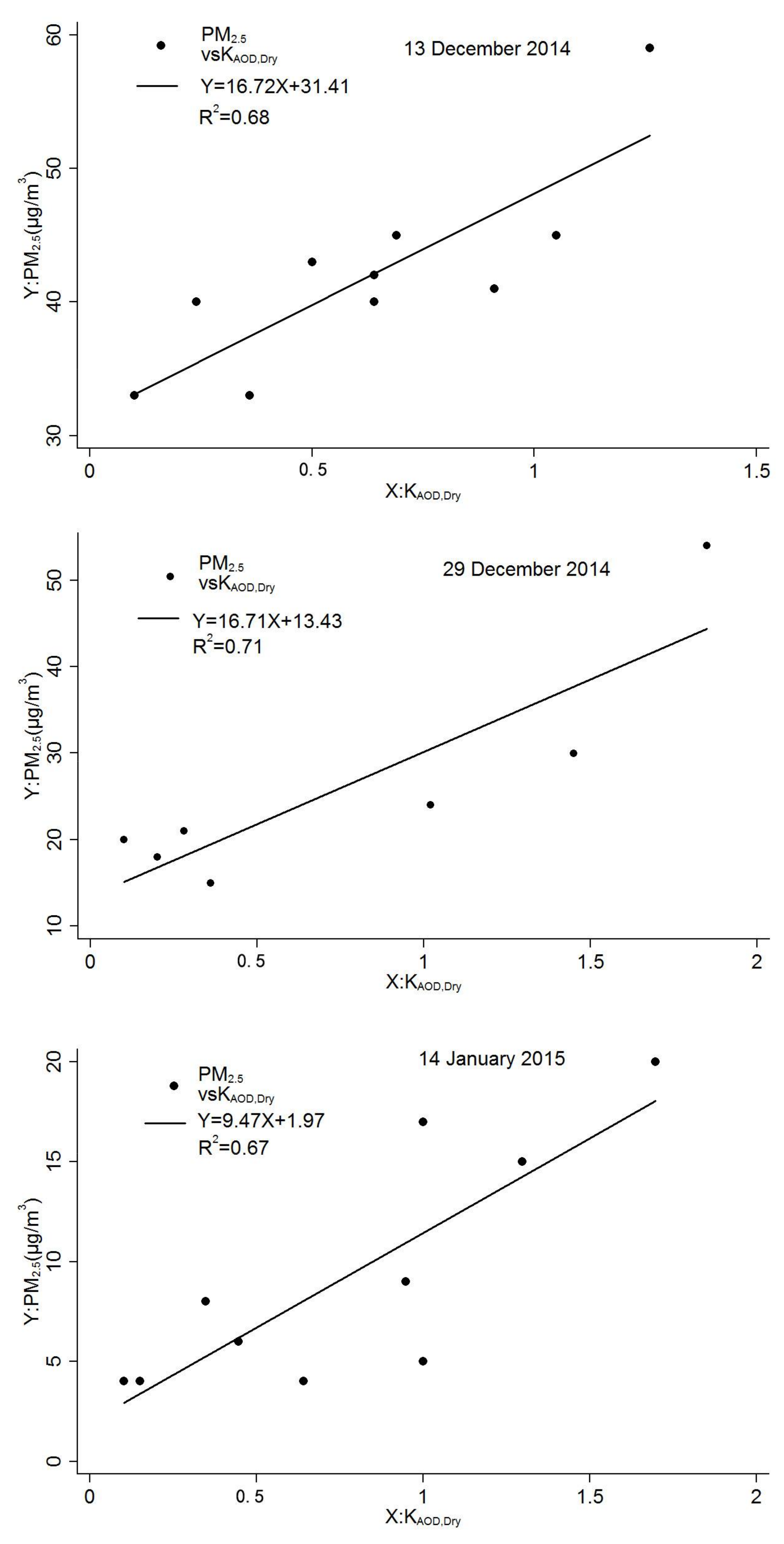
2.3.1. Satellite-Derived Aerosol Optical Depth (AOD)

We assumed that the land surface could be represented as a Lambert surface and that the atmospheric level was uniform. Apparent reflectance (${\rho }_{toa}$) at the top of the atmosphere can be expressed as [21]

$${\rho }_{toa}\left({\theta }_s,{\theta }_v,\varphi \right)={\rho }_0\left({\theta }_s,{\theta }_v,\varphi \right)+T\left({\theta }_s\right)·T\left({\theta }_v\right)·\frac{{\rho }_s\left({\theta }_s,{\theta }_v,\varphi \right)}{\left[1-{\rho }_s\left({\theta }_s,{\theta }_v,\varphi \right)·S\right]}$$

(1)

where ${\theta }_s$ is the solar zenith angle; ${\theta }_v$ is the satellite zenith angle; $\varphi$ is the azimuth of the scattered radiation from the solar beam; ${\rho }_0$ is path radiance; ${\rho }_s$ is the angular surface reflectance; $S$ is the atmospheric backscattering ratio; $T\left({\theta }_s\right)$ is the normalized downward flux for zero surface reflectance; and $T\left({\theta }_v\right)$ represents upward total transmission into the satellite’s field of view. We downloaded Landsat-8 data from the Geospatial Data Cloud (http://www.gscloud.cn) and then used ENVI5.3 software to preprocess the imagery. The pretreatment process mainly included masking, radiation calibration, geometric correction, and calculating the apparent reflectance $\left({\rho }_{toa}\right)$ of the atmosphere. The mid-infrared (2.12 mm) channel is less sensitive to aerosol scattering (because the wavelengths are larger than the size of most aerosol particles); however, the channels are sensitive to ground surface characteristics [22] and the apparent reflectance of mid-infrared at the top of the atmosphere, the angular surface reflectance of the red band, and the angular surface reflectance of the blue band have a fixed function, this function was modified using a Dark Dense Vegetation (DDV) algorithm [23]. Next, we used the DDV algorithm to calculate the surface reflectance of the red and blue bands. An aerosol lookup table (LUT) was constructed using the Second Simulation of the Satellite Signal in the Solar Spectrum (6S) atmosphere transmission model for the blue and red bands [21]. Finally, we obtained the atmospheric status of the computed reflectance which best matched the apparent reflectance of the atmosphere and the corresponding AOD value [22].

2.3.2. Calculation of PM_2.5 from AOD Data

AOD values indicate the accumulation of the extinction coefficient in the entire atmospheric column. The PM_2.5 concentrations only represent the near-surface “dry” aerosol extinction coefficient. An estimate of PM_2.5 concentrations from AOD data alone would produce large uncertainties. Therefore, we had to account for changes in PM_2.5 concentrations with elevation and correct for relative humidity in order to reduce these uncertainties [24]. Vertical and humidity corrections are needed to calculate PM_2.5 concentrations in urban forests from AOD data. To do this, the Height of Planetary Boundary Layer (HPBL) was incorporated into the vertical correction, while the effects of hygroscopic growth were used to determine the humidity correction [25,26]. In this study, AOD data were converted to a near-surface “dry” aerosol extinction coefficient and their correlation relationships with ground PM_2.5 concentrations [27,28]. The correlation between AOD and the surface aerosol extinction coefficient was affected by the vertical distribution of aerosols, so we determined the vertical correction for PM_2.5 concentrations using horizontal visibility to calculate the surface aerosol extinction coefficient. We also needed to correct for humidity because the meteorological stations measured PM_2.5 concentrations at a specific relative humidity, so we used relative humidity data to calculate the “dry” aerosol extinction coefficient. Next, we performed module estimations. Wang [29] found that it was possible to develop linear correlative models between a “dry” aerosol extinction coefficient and PM_2.5 concentration. We used the “dry” aerosol extinction coefficient and PM_2.5 concentrations collected in real time (at twelve ground monitoring sites) to establish models based on their correlation and estimate PM_2.5 concentrations. Our results indicated that the Landsat estimation of PM_2.5 correlates with ground-based measurements on 13 December 2014, 29 December 2014, and 14 January 2015, with R² = 0.68, 0.66, and 0.72, respectively (Figure 1). For additional details, please see Supplementary Materials.

2.4. Spatial Statistical Analysis

We used Global Moran’s I spatial autocorrelation method to determine the value of the relationship between a feature’s location and its attributes. We used the Getis-Ord Gi* spatial statistical method to provide us with a set of weighted values and identify statistically significant hot spots and cold spots on the ground. (Hot spots represent positions of statistically significant clustering of high PM_2.5 concentrations (p-value < 0.05) and cold spots represent positions of statistically significant clustering of low PM_2.5 concentrations (p-value < 0.05) [30]). Both Moran’s I and Getis-Ord Gi* have been used in a variety of ways, such as for helping to predict urban development patterns, analyzing pollution patterns, and examining traffic accident patterns [31,32]. We used the Moran’s I index to first analyze the spatial autocorrelation of PM_2.5. We then used the Getis-Ord Gi* index to identify areas of aggregated PM_2.5 (hot spots and cold spots). However, the Getis-Ord Gi* module demands that optimal threshold distances (i.e., distances at which spatial processes that promote clustering are most obvious) be supplied before it can analyze spatial data. Therefore, we used the incremental spatial autocorrelation module to determine the optimal distance threshold for aggregated areas [33]. Measures of spatial autocorrelation for a range of distances and optimal distances establish a line graph for those distances and their corresponding z-scores. Z-scores demonstrate the intensity of spatial clustering. However, statistically significant peak z-scores reveal distances where the spatial processes that promote clustering are most obvious. We used the incremental spatial autocorrelation module to determine the optimal distance threshold by increasing the threshold distance from 500 to 7000 m at intervals of 500 m until it reached its maximum value (3500 m). Therefore, we defined 3500 m as the optimal distance threshold in our study.

2.5. Geographical Detector Model Description

The geographical detector is a statistical tool for detecting spatially stratified heterogeneity and revealing the factors responsible for the heterogeneity [34]. In our study, we used a range of detectors designed to assess ecological and anthropogenic factors associated with PM_2.5 concentrations as determined by spatial variance analysis (SVA). The fundamental idea of SVA is to measure the spatial consistency of PM_2.5 concentration distribution versus ecological factors (e.g., forest, soils, topography) and anthropogenic factors (e.g., population density). The power of determinant (PD) of different impact factors on PM_2.5 concentration can be expressed using Equation (2):

$$\mathrm{PD}=1-\frac{1}{N\ast {\sigma }^2}{{\displaystyle \sum }}_{i=1}^L{N}_i\ast {\sigma }_i{}^2.$$

(2)

A detailed explanation of Equation (2) is as follows:

$$\mathrm{PD}=\mathrm{q}=1-\frac{{{\displaystyle \sum }}_{h=1}^l{{\displaystyle \sum }}_{i=1}^{N_h}{(Y_{hi}-{\overline{Y}}_h)}^2}{{{\displaystyle \sum }}_{i=1}^N{\left(Y_i-\overline{Y}\right)}^2}=1-\frac{{{\displaystyle \sum }}_{h=1}^l{N}_h{\sigma }_h^2}{N{\mathsf{\sigma }}^2}=1-\frac{SSW}{SST}$$

(3)

where the total sum of squares is

$$SST={\displaystyle \sum }_i^N{\left(Y_i-\overline{Y}\right)}^2=N{\mathsf{\sigma }}^2$$

(4)

and the sum of squares within is

$$SSW={{\displaystyle \sum }}_{h=1}^l{\displaystyle \sum }_i^{N_h}{(Y_{hi}-{\overline{Y}}_h)}^2={\displaystyle \sum }_{h=1}^l{N}_h{\sigma }_h^2$$

(5)

where $\mathrm{PD}$ is the power of determinant of impact factors on PM_2.5 concentration; $\underset{¯}{N}$ is the number of forest patches and is stratified into $h=1,\dots ,2,L$ strata; stratum $h$ is composed of $N_h$ units; $Y_i$ and $Y_{hi}$ denote the value of unit $\underset{¯}{i}$ in the population and in stratum $\underset{¯}{h}$, respectively; the stratum mean is ${\overline{Y}}_h=(\frac{1}{N_h}){{\displaystyle \sum }}_{i=1}^{N_h}{Y}_{hi}$; the stratum variance is ${\sigma }_h^2$ = $\left(\frac{1}{N_h}\right){{\displaystyle \sum }}_i^{N_h}(Y_{hi}-Y_h)$²; the population mean is Y = $(\frac{1}{N_h}){{\displaystyle \sum }}_{i=1}^N{Y}_i$; and the population variance of PM_2.5 concentrations of the entire region is ${\sigma }^2=\left(\frac{1}{N_h}\right){{\displaystyle \sum }}_i^{N_h}(Y_i-Y$)². $\mathrm{PD}$ ∈ [0,1], where $\mathrm{PD}$ approaches 0, implies that the determinant is completely unrelated to the PM_2.5 concentrations. Where $\mathrm{PD}$ approaches 1, the determinant completely controls PM_2.5 concentration. $\mathrm{PD}$ has a corresponding p-value that can be used to evaluate uncertainty [35]. For additional details, please see Supplementary Materials. Based on this idea, we used geographical detector tools (factor detector and interaction detector) to detect various factors that may influence PM_2.5 concentrations, the degree of influence of each factor, and the interactions between factors based on spatial analysis of variance [36]. The factor detector quantifies the impact of ecological and anthropogenic factors on an observed spatial PM_2.5 pattern. The interaction detector probes whether two impact factors taken together enhance or weaken each other, or whether they affect PM_2.5 concentrations independently [37].

$$\mathrm{Enhance},\mathrm{nonlinear}:\mathrm{PD}\left(X_1\cap X_2=\mathrm{X}3\right)>\mathrm{PD}\left(X_1\right)+\mathrm{PD}\left(X_2\right),$$

(6)

$$\mathrm{Independent}:\mathrm{PD}\left(X_1\cap X_2=\mathrm{X}3\right)=\mathrm{PD}\left(X_1\right)+\mathrm{PD}\left(X_2\right),$$

(7)

$$\mathrm{Enhance},\mathrm{bi}:\mathrm{PD}\left(X_1\cap X_2=\mathrm{X}3\right)>Max(\mathrm{PD}\left(X_1\right),\mathrm{PD}\left(X_2\right),$$

(8)

where $X_1$, $X_2,$ and $\mathrm{X}3$ represent the impact factors. $\mathrm{PD}\left(X_1\right),\mathrm{PD}\left(X_2\right),$ and $\mathrm{PD}\left(X_1\cap X_2=\mathrm{X}3\right)$ are the power of determinants of the impact factors on PM_2.5 concentrations. $\mathrm{Max}\left(\mathrm{PD}\left(X_1\right),\mathrm{PD}\left(X_2\right)\right)$ represents the maximum value of $\mathrm{PD}\left(X_1\right),\mathrm{PD}\left(X_2\right)$. So, the PD value of each impact factor and the PD value of their interactions are used to quantitatively evaluate the relationships between potential impacts and their determinants. The geographical detector models used in this study are freely available from http://www.sssampling.org/Excel-geodetector/. According to the geographical detector input rules, all independent variables should be discrete. Therefore, the rules in the FMPI instruction manual and the natural breaks method were chosen as the classification method. Multiple environmental factors and population density were applied as independent variables in the geographical detector model. Specifically, PM_2.5 concentration is the dependent variable. We used geographical detector models to examine the individual and interactive effects of multiple ecological and anthropogenic factors on urban forest PM_2.5 concentrations.

3. Results

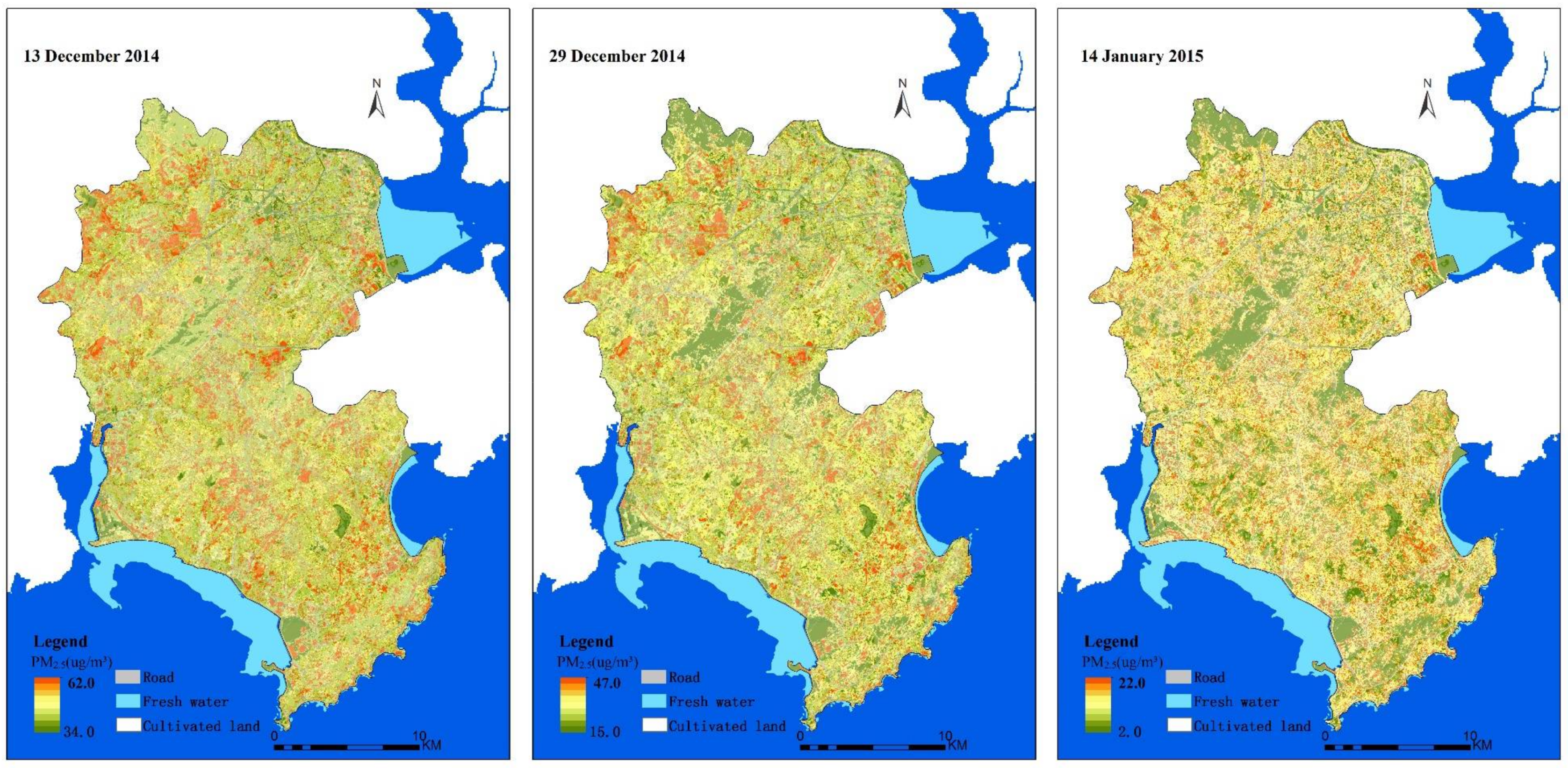
3.1. Spatial Distribution Pattern of Urban Forest PM_2.5 Concentrations

The spatial distributions of PM_2.5 concentrations on 13 and 29 December 2014 and 14 January 2015 showed significant spatial clustering (Global Moran’s I = 0.192, z-score = 63.412 on 13 December 2014; Global Moran’s I = 0.336, z-score = 110.860 on 29 December 2014; Global Moran’s I = 0.185, z-score = 95.761 on 14 January 2015) (

Table 1. The global spatial autocorrelation statistics (Moran’s I) of PM_2.5 concentrations on 13 December 2014, 29 December 2014, and 14 January 2015.

Time	13 December 2014	29 December 2014	14 January 2015
Moran’s I Index	0.192 **	0.336 **	0.185 **
z-score	63.412	110.860	95.761
Pattern	Clustered	Clustered	Clustered

Note: p < 0.001 in all regions in 2014 and 2015; ** represents significant values.

). The aggregated areas (hot spots and cold spots) of PM_2.5 identified by Getis-Ord Gi* showed that PM_2.5 hot spots were concentrated in urban centers and suburbs (n = 1917 on 13 December 2014; n = 2283 on 29 December 2014; n = 1887 on 14 January 2015) and cold spots were mainly distributed in the suburbs and exurban regions (n = 1082 on 13 December 2014; n = 1212 on 29 December 2014; n = 1337 on 14 January 2015) (Figure 2).

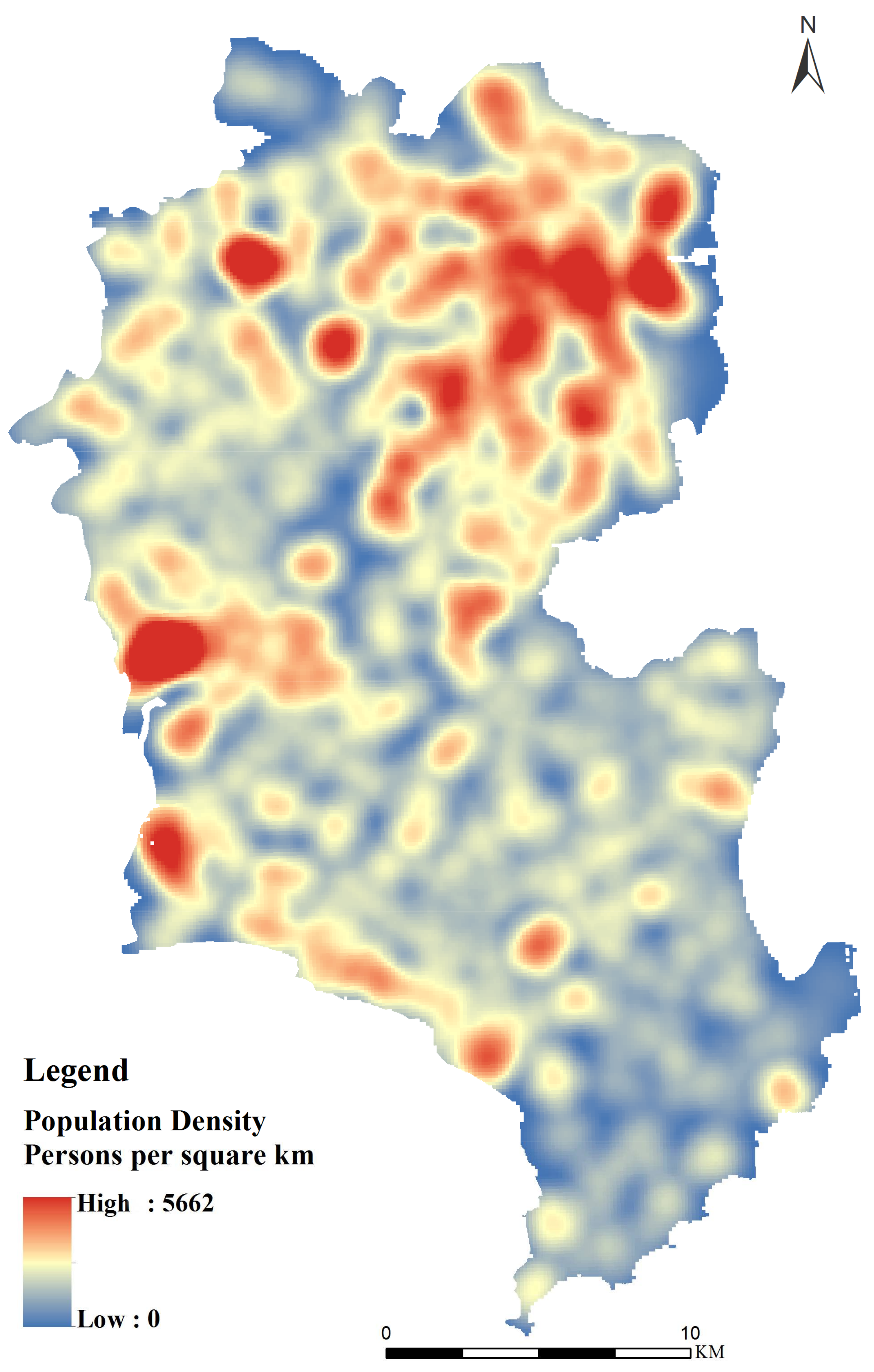
3.2. Population Density and Stand Structure

The human population density of Jinjiang was 1530 people km⁻² and the density distribution demonstrated a significant spatial autocorrelation (Moran’s I = 0.642, z-score = 269.293) in 2014 (Figure 3). The Getis-Ord Gi* statistics revealed that the spatial distributions of the population and PM_2.5 concentrations were similar in the northwest and on the central coast, but were different in the south. According to the FMPI data, the total area of forest in the study region was 9565.68 ha, average canopy density was 0.393, and average tree age was 20.123 ± 5.857 years. The dominant tree species in the urban forests were Casuarina pusilla, Acacia crassicapa, Eucalyptus robusta Smith, Acacia confusa Merr, Cunninghamia lanceolate, and Pinus massoniana.

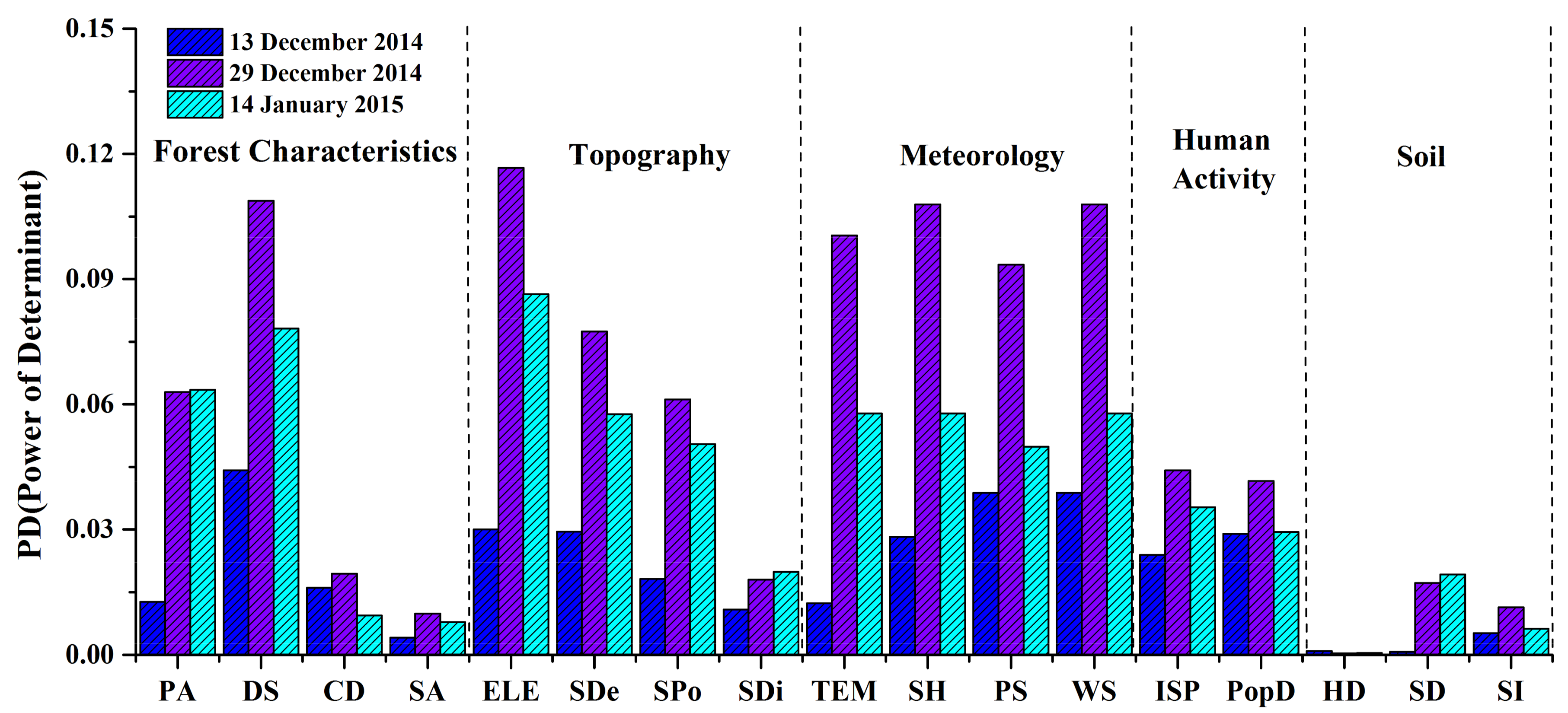
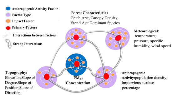
3.3. Influences of Anthropogenic and Ecological Factors on Urban Forest PM_2.5 Concentrations

We compared the locations of PM_2.5 hot and cold spots on three dates. Our results showed that elevation (a topographic factor), dominant tree species (a forest characteristic factor), and wind speed (a meteorological factor) were the main factors related to urban forest PM_2.5 concentrations. These three factors influenced the model more than population density (Figure 4,

Table 2. The power of determinant (PD) of forest attributes, soil, topography, meteorological factors, and population on PM_2.5 concentrations on three different days.

Factors	Factor Composition	13 December 2014	29 December 2014	14 January 2015
Forest Characteristics	PA	0.013	0.063	0.063
	DS	0.044	0.109	0.078
	CD	0.016	0.019	0.009
	SA	0.004	0.010	0.008
Soil	SI	0.005	0.011	0.006
	SD	0.001	0.017	0.019
	HD	0.001	0.001	0.001
Topography	ELE	0.030	0.117	0.086
	SDe	0.029	0.077	0.058
	SPo	0.018	0.061	0.050
	SDi	0.011	0.018	0.020
Human Activity	PopD	0.029	0.042	0.029
	ISP	0.024	0.044	0.035
Meteorological factors	TEM	0.012	0.100	0.057
	SH	0.028	0.107	0.057
	PS	0.038	0.093	0.049
	WS	0.038	0.107	0.057

). In addition, the interaction between elevation and dominant tree species showed enhancement as did the interaction between elevation and impervious surface percentage. Dominant tree species and population density showed enhancement as did dominant tree species and impervious surface percentage. The influence of ecological factors on the model differed among the three dates. For example, on 13 December 2014, the main influential factors were dominant tree species (PD = 0.044), wind speed (PD = 0.038), and elevation (PD = 0.030). On 29 December 2014, the main influential factors were elevation (PD = 0.108), wind speed (PD = 0.107), and dominant tree species (PD = 0.103). On 14 January 2015, the main influential factors were elevation (PD = 0.077), dominant tree species (PD = 0.075), and forest patch area (PD = 0.063). Compared with the independent effect of population density, the interactive effect was significant. Although the independent effect of population density was weak, we cannot simply assume that population density was not crucial. Spatial heterogeneity is complex in urban environments and human activities have a significant impact on urban ecosystems. The interactive effect could be more than the sum of the independent effects of any two factors. For example, the interactive effect of dominant tree species and population density (0.154) is greater than the sum of the individual effects of dominant tree species and population density (0.071). With the acceleration of urbanization, the interactive effects of population density, impervious surface percentage, and other factors could result in increased air pollution (Figure 5). The datasets in this study were limited by the availability of remote sensing image archives and the cloud-prone climate in southern China, which allowed us to select only three qualified scenes (i.e., 13 December 2014, 29 December 2014, and 14 January 2015) under relatively clear and stable atmospheric conditions.

4. Discussion

4.1. Significance

Integration of Landsat images and multisource data using spatial statistical analysis and a geographical detector model can reveal the individual and interactive influences of anthropogenic and ecological factors on PM_2.5 concentrations. The results of this study emphasize the importance of human activities and ecological factors in determining PM_2.5 concentrations and the different strengths of these factors. Our study provides a more comprehensive analysis of human and ecological influencing factors through the use of remote sensing data, statistical analysis, and monitoring data at an urban scale.

4.2. Individual Functions

The ecological factors of elevation, dominant tree species, and meteorological factors significantly influenced particulate concentrations in urban areas. Many studies have shown that, at small spatial scales, elevation affects particulate concentrations by influencing air flow, pressure, temperature, and precipitation [38,39]. There are several possible explanations for this finding: (1) Particulates are more buoyant in the air at low elevation (over time, PM_2.5 at high elevations will sink down to low elevations, adding to the concentration of PM_2.5 at the lower elevation); (2) Each 100 m increase in elevation coincides with a 0.6 °C drop in temperature, which affects particulate concentrations [40]. At higher elevations, the ground absorbs more radiation from the sun, which warms air near the ground and causes it to rise, creating convection currents in the upper atmosphere. This meteorological process encourages the proliferation of atmospheric pollutants (including particulates); (3) As atmospheric pressure decreases with increasing elevation [41,42], air volume expands and the atmosphere becomes less stable, thus leading to a widespread diffusion of air pollutants.

Tree species composition significantly affected particulate concentrations, presumably because the dust-removing ability of plants differs significantly by species [43,44]. The variations in particulate retention among tree species in this study were consistent with those found by Liu [12] and Yang [45] and may be explained by variations in morphological characteristics that enable plants to trap particulates (e.g., canopy structure, leaf density, leaf surface roughness, and wax) [16]. The three-dimensional structure of tree canopies encourages turbulent air movement and the more complex the canopy structure, the more particulates are deposited onto leaf surfaces [46]. Conifers retain more particulates than broadleaf trees because of their smaller, more densely packed leaves and more complex stem arrangements [47]. Rough leaf surfaces are also more effective than smooth leaf surfaces in accumulating particulates [48].

Wind speed is also an important factor affecting the diffusion of PM_2.5 concentrations. In general, higher wind speeds contribute to PM_2.5 diffusion. Under zero wind speed conditions, PM_2.5 particulates aggregated at the surface layer [49].

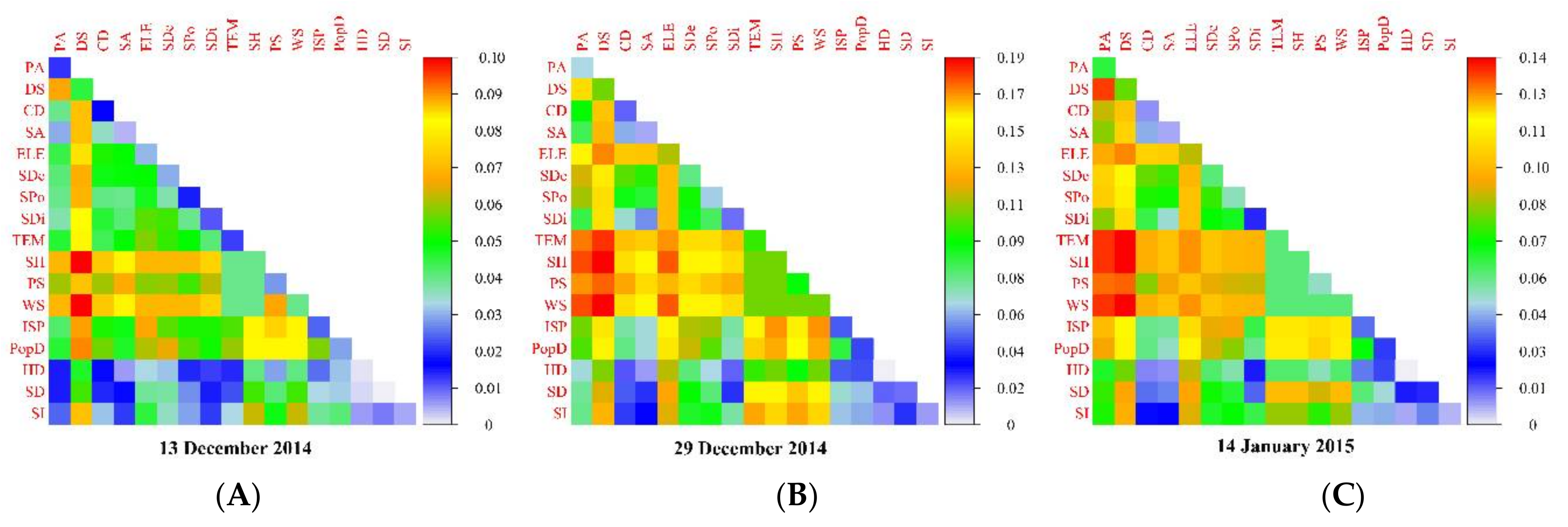
4.3. Interactive Functions

Our study found that human activities significantly enhanced the effects of ecological factors on PM_2.5 concentrations. This suggests that human activities might be the dominant factor affecting PM_2.5 concentrations in Jinjiang, China, which is consistent with previous research [50]. Of the anthropogenic factors, we found that population density was most responsible for enhancing the effects of elevation and dominant tree species on PM_2.5 concentrations. The increase in population density caused by increased residential areas and increased impervious surface percentage could significantly increase the PM_2.5 concentrations in central urban areas [51]. Populations and industries tend to settle and build at low elevations. The resulting heavy human and industrial activity could therefore significantly increase PM_2.5 concentrations in central urban areas [52]. The interactive effects between impervious surface percentage and other factors were similar to those just described for population density. These findings show that the combined influences of anthropogenic activities and multiple ecological factors on PM_2.5 concentrations should be considered when developing pollution monitoring and control strategies in Jinjiang, China. Previous studies used multivariate statistics to study the individual impacts of multiple ecological factors (such as tree species composition, NDVI, etc.) on PM_2.5 concentrations [53,54]. However, these studies ignored the interactions of these factors. Furthermore, multivariate statistical analyses have not considered the spatial heterogeneity of PM_2.5 concentrations and have only focused on nonspatial features and attributes. Thus, we used geographical detector models to examine the individual and interactive influences of anthropogenic and ecological factors. This approach assesses the multiple ecological and anthropogenic factors associated with PM_2.5 concentrations by means of spatial variance analysis (SVA).

4.4. Limitations and Advantages of the Study

There are several limitations of the present study. First, the correlation between AOD and particulates was complex. We found that it varied at different temporal and spatial scales. In the future, we need to improve our understanding of the chemical properties of AOD and particulates to improve the model’s accuracy. Second, because the urban ecosystem is complex and factors that affect pollution in cities differ spatially, we need to identify functional areas (e.g., clean areas, traffic areas, industrial areas) and study the different dust-retention mechanisms within them. Third, because of data limitations, the anthropogenic factors included only population density and impervious surface percentage, which cannot comprehensively express the characteristics of human activities. Fourth, future research should focus on integrating longer time series of remote sensing images to more accurately delineate the interactions between multiple ecological factors and their effects on urban forest PM_2.5 concentrations, while also using remote sensing data fusion methods to achieve high temporal and spatial resolution simultaneously at the city scale. Finally, the process of comparing quantitative impact factors with qualitative impact factors is subjective, because arbitrary methods of discretization (e.g., standard deviation, equal interval, Jenks, and quantile) may not characterize the actual associations between impact factors and PM_2.5 concentrations [55,56,57].

Despite these limitations, this study has several advantages. First, we integrated detailed datasets (including FMPI, Landsat-8 images, population density distribution data, topographic data, and meteorological data). Second, we analyzed the spatial distribution of PM_2.5 concentrations and described their spatial heterogeneity. Finally, we revealed the individual and interactive influences of anthropogenic and ecological factors on PM_2.5 concentrations, which improves our understanding of PM_2.5 pollution distribution patterns in Jinjiang, China.

5. Conclusions

At present, most studies of PM_2.5 concentrations are conducted at large spatial scales, have a broad research scope, and use remote sensing images with coarse image resolution. Here, we focus on urban ecosystems, using a case study to create a methodology for quantifying the interactions between human activities and multiple ecological factors at an urban scale. Our method reveals the individual and interactive influences of these factors on PM_2.5 concentrations by integrating field surveys with satellite-derived PM_2.5 data and population density data. We used a spatial statistical analysis model to identify aggregated areas (hot spots and cold spots) of particulates in an urban environment. A geographic detector model was used to quantify the impact of ecological and anthropogenic factors on observed spatial PM_2.5 patterns and to probe whether two impact factors enhance, weaken, or remain independent of each other when considering their combined impacts on PM_2.5 concentrations. FMPI can provide vegetation attribute information (e.g., forest, soil, topography, and other attribute information) and model input parameters. Spatial statistics describe the spatial heterogeneity of particulate concentrations. We found that fine particulate concentration hot spots are mainly distributed in urban centers and suburbs, while cold spots are mainly distributed in the suburbs and exurban regions. Elevation was the dominant individual factor affecting PM_2.5 concentrations, followed by dominant tree species and meteorological factors. In terms of interactive effects, the combination of human activities (e.g., population density, impervious surface percentage) and multiple ecological factors led to the largest increases in PM_2.5 concentrations in our study area. In conclusion, in order to reveal the direct and indirect effects of human activities and multiple factors on PM_2.5 concentrations in urban forests, quantification of fusion satellite data and spatial statistical methods should be conducted in urban areas. These findings extend our understanding of the factors influencing the spatial distribution of PM_2.5 concentrations and may help guide efforts to manage air pollution, monitor pollution, and estimate pollution exposure.

References

1. Wu, J.S.; Yao, F.; Li, W.F.; Si, M.L. Viirs-based remote sensing estimation of ground-level PM2.5 concentrations in beijing-tianjin-hebei: A spatiotemporal statistical model. Remote Sens. Environ. 2016, 184, 316–328. [Google Scholar] [CrossRef]
2. Pope, C.A.; Burnett, R.T.; Thun, M.J.; Calle, E.E.; Krewski, D.; Ito, K.; Thurston, G.D. Lung cancer, cardiopulmonary mortality, and long-term exposure to fine particulate air pollution. J. Am. Med. Assoc. 2002, 287, 1132–1141. [Google Scholar] [CrossRef]
3. Kappos, A.D.; Bruckmann, P.; Eikmann, T.; Englert, N.; Heinrich, U.; Hoppe, P.; Koch, E.; Krause, G.H.M.; Kreyling, W.G.; Rauchfuss, K.; et al. Health effects of particles in ambient air. Int. J. Hyg. Environ. Health 2004, 207, 399–407. [Google Scholar] [CrossRef] [PubMed]
4. Solomon, S.; Qin, D.; Manning, M.; Chen, Z.; Marquis, M.; Averyt, K.B.; Tignor, M.; Miller, H.L. Contribution of Working Group I to the Fourth Assessment Report of the Intergovernmental Panel on Climate Change, 2007; Cambridge University Press: Cambridge, UK; New York, NY, USA, 2007; p. 976. [Google Scholar]
5. Liu, Z.; Sun, Y.; Li, L.; Wang, Y. Particle mass concentrations and size distribution during and after the Beijing Olympic games. Huan jing ke xue = Huanjing kexue 2011, 32, 913–923. [Google Scholar] [PubMed]
6. Chen, B.; Lu, S.W.; Zhao, Y.G.; Li, S.N.; Yang, X.B.; Wang, B.; Zhang, H.J. Pollution remediation by urban forests: PM2.5 reduction in Beijing, China. Pol. J. Environ. Stud. 2016, 25, 1873–1881. [Google Scholar] [CrossRef]
7. Rissanen, T.; Hyotylainen, T.; Kallio, M.; Kronholm, J.; Kulmala, M.; Rikkola, M.L. Characterization of organic compounds in aerosol particles from a coniferous forest by GC-MS. Chemosphere 2006, 64, 1185–1195. [Google Scholar] [CrossRef] [PubMed]
8. Pio, C.; Alves, C.; Duarte, A. Organic components of aerosols in a forested area of central Greece. Atmos. Environ. 2001, 35, 389–401. [Google Scholar] [CrossRef]
9. Tiwary, A.; Sinnett, D.; Peachey, C.; Chalabi, Z.; Vardoulakis, S.; Fletcher, T.; Leonardi, G.; Grundy, C.; Azapagic, A.; Hutchings, T.R. An integrated tool to assess the role of new planting in PM10 capture and the human health benefits: A case study in London. Environ. Pollut. 2009, 157, 2645–2653. [Google Scholar] [CrossRef] [PubMed]
10. Gagne, S.A.; Sherman, P.J.; Singh, K.K.; Meentemeyer, R.K. The effect of human population size on the breeding bird diversity of urban regions. Biodivers. Conserv. 2016, 25, 653–671. [Google Scholar] [CrossRef]
11. Jin, S.J.; Guo, J.K.; Wheeler, S.; Kan, L.Y.; Che, S.Q. Evaluation of impacts of trees on PM2.5 dispersion in urban streets. Atmos. Environ. 2014, 99, 277–287. [Google Scholar] [CrossRef]
12. Liu, X.H.; Yu, X.X.; Zhang, Z.M. PM2.5 concentration differences between various forest types and its correlation with forest structure. Atmosphere 2015, 6, 1801–1815. [Google Scholar] [CrossRef]
13. Shu, J.; Dearing, J.A.; Morse, A.P.; Yu, L.Z.; Yuan, N. Determining the sources of atmospheric particles in Shanghai, China, from magnetic and geochemical properties. Atmos. Environ. 2001, 35, 2615–2625. [Google Scholar] [CrossRef]
14. Gao, G.J.; Sun, F.B.; Thao, N.T.T.; Lun, X.X.; Yu, X.X. Different concentrations of TSP, PM10, PM2.5, and PM1 of several urban forest types in different seasons. Pol. J. Environ. Stud. 2015, 24, 2387–2395. [Google Scholar] [CrossRef]
15. Hu, Y.; Xia, C.; Li, S.; Ward, M.P.; Luo, C.; Gao, F.; Wang, Q.; Zhang, S.; Zhang, Z. Assessing environmental factors associated with regional schistosomiasis prevalence in Anhui province, Peoples’ Republic of China using a geographical detector method. Infect. Dis. Poverty 2017, 6, 87. [Google Scholar] [CrossRef] [PubMed]
16. Saebo, A.; Popek, R.; Nawrot, B.; Hanslin, H.M.; Gawronska, H.; Gawronski, S.W. Plant species differences in particulate matter accumulation on leaf surfaces. Sci. Total Environ. 2012, 427, 347–354. [Google Scholar] [CrossRef] [PubMed]
17. Ord, J.K.; Getis, A. Local spatial autocorrelation statistics: Distributional issues and an application. Geogr. Anal. 1995, 27, 286–306. [Google Scholar] [CrossRef]
18. Barrell, J.; Grant, J. Detecting hot and cold spots in a seagrass landscape using local indicators of spatial association. Landsc. Ecol. 2013, 28, 2005–2018. [Google Scholar] [CrossRef]
19. Lei, X.D.; Tang, M.P.; Lu, Y.C.; Hong, L.X.; Tian, D.L. Forest inventory in China: Status and challenges. Int. For. Rev. 2009, 11, 52–63. [Google Scholar] [CrossRef]
20. He, J.; Yang, K. China Meteorological Forcing Dataset; Cold and Arid Regions Science Data Center at Lanzhou: Lanzhou, China, 2011; Available online: http://westdc.westgis.ac.cn/data/7a35329c-c53f-4267-aa07-e0037d913a21 (accessed on 1 March 2018).
21. Vermote, E.F.; Tanre, D.; Deuze, J.L.; Herman, M.; Morcrette, J.J. Second simulation of the satellite signal in the solar spectrum, 6s: An overview. IEEE Trans. Geosci. Remote Sens. 1997, 35, 675–686. [Google Scholar] [CrossRef]
22. Chen, Y.P.; Han, W.H.; Chen, S.Z.; Tong, L. Estimating ground-level PM2.5 concentration using Landsat 8 in Chengdu, China. In Remote Sensing of the Atmosphere, Clouds, and Precipitation v; Im, E., Yang, S., Zhang, P., Eds.; SPIE: Bellingham, WA, USA, 2014; Volume 9259. [Google Scholar]
23. Levy, R.C.; Remer, L.A.; Mattoo, S.; Vermote, E.F.; Kaufman, Y.J. Second-generation operational algorithm: Retrieval of aerosol properties over land from inversion of moderate resolution imaging spectroradiometer spectral reflectance. J. Geophys. Res. Atmos. 2007, 112. [Google Scholar] [CrossRef]
24. Koelemeijer, R.B.A.; Homan, C.D.; Matthijsen, J. Comparison of spatial and temporal variations of aerosol optical thickness and particulate matter over Europe. Atmos. Environ. 2006, 40, 5304–5315. [Google Scholar] [CrossRef]
25. Lin, C.Q.; Li, Y.; Yuan, Z.B.; Lau, A.K.H.; Li, C.C.; Fung, J.C.H. Using satellite remote sensing data to estimate the high-resolution distribution of ground-level PM2.5. Remote Sens. Environ. 2015, 156, 117–128. [Google Scholar] [CrossRef]
26. He, Q.S.; Li, C.C.; Geng, F.H.; Zhou, G.Q.; Gao, W.; Yu, W.; Li, Z.K.; Du, M.B. A parameterization scheme of aerosol vertical distribution for surface-level visibility retrieval from satellite remote sensing. Remote Sens. Environ. 2016, 181, 1–13. [Google Scholar] [CrossRef]
27. Jung, J.; Lee, H.; Kim, Y.J.; Liu, X.; Zhang, Y.; Gu, J.; Fan, S. Aerosol chemistry and the effect of aerosol water content on visibility impairment and radiative forcing in Guangzhou during the 2006 Pearl River Delta campaign. J. Environ. Manag. 2009, 90, 3231–3244. [Google Scholar] [CrossRef] [PubMed]
28. Huang, W.X.; Cheng, X.W. Multiple regression method for estimating concentration of PM2.5 using remote sensing and meteorological data. J. Environ. Prot. Ecol. 2017, 18, 417–424. [Google Scholar]
29. Wang, Z.F.; Chen, L.F.; Tao, J.H.; Zhang, Y.; Su, L. Satellite-based estimation of regional particulate matter (PM) in Beijing using vertical-and-RH correcting method. Remote Sens. Environ. 2010, 114, 50–63. [Google Scholar] [CrossRef]
30. Eck, J.; Chainey, S.; Cameron, J.; Wilson, R. Mapping Crime: Understanding Hotspots; U.S. Department of Justice, Office of Justice Programs: Washington, DC, USA, 2005.
31. Kara, C.; Akcit, N. Traffic accident analysis using Gis: A case study of Kyrenia city. In Third International Conference on Remote Sensing and Geoinformation of the Environment; Hadjimitsis, D.G., Themistocleous, K., Michaelides, S., Papadavid, G., Eds.; SPIE: Bellingham, WA, USA, 2015; Volume 9535. [Google Scholar]
32. Mei, Z.X.; Xu, S.J.; Ouyang, J. Spatio-temporal association analysis of county potential in the Pearl River Delta during 1990–2009. J. Geogr. Sci. 2015, 25, 319–336. [Google Scholar] [CrossRef]
33. Stopka, T.J.; Krawczyk, C.; Gradziel, P.; Geraghty, E.M. Use of spatial epidemiology and hot spot analysis to target women eligible for prenatal women, infants, and children services. Am. J. Public Health 2014, 104, S183–S189. [Google Scholar] [CrossRef] [PubMed]
34. Hu, Y.; Wang, J.; Li, X.; Ren, D.; Zhu, J. Geographical detector-based risk assessment of the under-five mortality in the 2008 Wenchuan Earthquake, China. PLoS ONE 2011, 6, e21427. [Google Scholar] [CrossRef] [PubMed]
35. Du, Z.Q.; Xu, X.M.; Zhang, H.; Wu, Z.T.; Liu, Y. Geographical detector-based identification of the impact of major determinants on Aeolian Desertification Risk. PLoS ONE 2016, 11, e0151331. [Google Scholar] [CrossRef] [PubMed]
36. Wang, J.F.; Li, X.H.; Christakos, G.; Liao, Y.L.; Zhang, T.; Gu, X.; Zheng, X.Y. Geographical detectors-based health risk assessment and its application in the neural tube defects study of the Heshun region, China. Int. J. Geogr. Inf. Sci. 2010, 24, 107–127. [Google Scholar] [CrossRef]
37. Cao, Z.; Liu, T.; Li, X.; Wang, J.; Lin, H.L.; Chen, L.L.; Wu, Z.F.; Ma, W.J. Individual and interactive effects of socio-ecological factors on dengue fever at fine spatial scale: A geographical detector-based analysis. Int. J. Environ. Res. Public Health 2017, 14, 795. [Google Scholar] [CrossRef] [PubMed]
38. Zhang, T.H.; Liu, G.; Zhu, Z.M.; Gong, W.; Ji, Y.X.; Huang, Y.S. Real-time estimation of satellite-derived PM2.5 based on a semi-physical geographically weighted regression model. Int. J. Environ. Res. Public Health 2016, 13, 974. [Google Scholar] [CrossRef] [PubMed]
39. Cisneros, R.; Schweizer, D.; Preisler, H.; Bennett, D.H.; Shaw, G.; Bytnerowicz, A. Spatial and seasonal patterns of particulate matter less than 2.5 microns in the sierra Nevada Mountains, California. Atmos. Pollut. Res. 2014, 5, 581–590. [Google Scholar] [CrossRef]
40. Halsey, L.A.; Vitt, D.H.; Zoltai, S.C. Disequilibrium response of permafrost in boreal continental Western Canada to climate change. Clim. Chang. 1995, 30, 57–73. [Google Scholar] [CrossRef]
41. Stone, J.O. Air pressure and cosmogenic isotope production. J. Geophys. Res.-Solid Earth 2000, 105, 23753–23759. [Google Scholar] [CrossRef]
42. Körner, C. The use of ‘altitude’ in ecological research. Trends Ecol. Evol. 2007, 22, 569–574. [Google Scholar] [CrossRef] [PubMed]
43. Zhang, Z.M.; Liu, J.K.; Wu, Y.N.; Yan, G.X.; Zhu, L.J.; Yu, X.X. Multi-scale comparison of the fine particle removal capacity of urban forests and wetlands. Sci. Rep. 2017, 7, 46214. [Google Scholar] [CrossRef] [PubMed]
44. Nguyen, T.; Yu, X.X.; Zhang, Z.M.; Liu, M.M.; Liu, X.H. Relationship between types of urban forest and PM2.5 capture at three growth stages of leaves. J. Environ. Sci. 2015, 27, 33–41. [Google Scholar] [CrossRef] [PubMed]
45. Yang, J.; Xie, B.Z.; Shi, H.; Wang, H.X.; Wang, Y.H. Study on capturing PM2.5 capability of tree species in different functional areas. In Proceedings of the 2015 International Conference on Industrial Technology and Management Science; Zhao, J., Ed.; Atlantis Press: Paris, France, 2015; Volume 34, pp. 585–588. [Google Scholar]
46. Fowler, D.; Cape, J.N.; Unsworth, M.H. Deposition of atmospheric pollutants on forests. Philos. Trans. R. Soc. Lond. Ser. B Biol. Sci. 1989, 324, 247–265. [Google Scholar] [CrossRef]
47. Beckett, K.P.; Freer-Smith, P.H.; Taylor, G. Urban woodlands: Their role in reducing the effects of particulate pollution. Environ. Pollut. 1998, 99, 347–360. [Google Scholar] [CrossRef]
48. Hwang, H.-J.; Yook, S.-J.; Ahn, K.-H. Experimental investigation of submicron and ultrafine soot particle removal by tree leaves. Atmos. Environ. 2011, 45, 6987–6994. [Google Scholar] [CrossRef]
49. Kim, K.H.; Kim, M.Y.; Hong, S.M.; Youn, Y.H.; Hwang, S.J. The effects of wind speed on the relative relationships between different sized-fractions of airborne particles. Chemosphere 2005, 59, 929–937. [Google Scholar] [CrossRef] [PubMed]
50. Lou, C.R.; Liu, H.Y.; Li, Y.F.; Li, Y.L. Socioeconomic drivers of PM2.5 in the accumulation phase of air pollution episodes in the Yangtze River Delta of China. Int. J. Environ. Res. Public Health 2016, 13, 928. [Google Scholar] [CrossRef] [PubMed]
51. Beelen, R.; Hoek, G.; Pebesma, E.; Vienneau, D.; de Hoogh, K.; Briggs, D.J. Mapping of background air pollution at a fine spatial scale across the European Union. Sci. Total Environ. 2009, 407, 1852–1867. [Google Scholar] [CrossRef] [PubMed]
52. Hoek, G.; Beelen, R.; de Hoogh, K.; Vienneau, D.; Gulliver, J.; Fischer, P.; Briggs, D. A review of land-use regression models to assess spatial variation of outdoor air pollution. Atmos. Environ. 2008, 42, 7561–7578. [Google Scholar] [CrossRef]
53. Beckett, K.P.; Freer-Smith, P.H.; Taylor, G. Particulate pollution capture by urban trees: Effect of species and windspeed. Glob. Chang. Biol. 2000, 6, 995–1003. [Google Scholar] [CrossRef]
54. Baxter, L.K.; Burke, J.; Lunden, M.; Turpin, B.J.; Rich, D.Q.; Thevenet-Morrison, K.; Hodas, N.; Ozkaynak, H. Influence of human activity patterns, particle composition, and residential air exchange rates on modeled distributions of PM2.5 exposure compared with central-site monitoring data. J. Expo. Sci. Environ. Epidemiol. 2013, 23, 241–247. [Google Scholar] [CrossRef] [PubMed]
55. Bai, H.; Li, D.; Ge, Y.; Wang, J. Detecting nominal variables’ spatial associations using conditional probabilities of neighboring surface objects’ categories. Inf. Sci. 2016, 329, 701–718. [Google Scholar] [CrossRef]
56. Tang, L.N.; Shao, G.F.; Piao, Z.J.; Dai, L.M.; Jenkins, M.A.; Wang, S.X.; Wu, G.; Wu, J.G.; Zhao, J.Z. Forest degradation deepens around and within protected areas in east Asia. Biol. Conserv. 2010, 143, 1295–1298. [Google Scholar] [CrossRef]
57. Zhao, J.Z.; Liu, X.; Dong, R.C.; Shao, G.F. Landsenses ecology and ecological planning towards sustainable development. Int. J. Sustain. Dev. World Ecol. 2016, 23, 293–297. [Google Scholar] [CrossRef]
Figure 1. Correlation between k A O D , D r y and PM2.5 concentrations on 13 December 2014, 29 December 2014, and 14 January 2015 (both acquired from Environmental Protection of Jinjiang k A O D , D r y represents the aerosol extinction coefficient in dry conditions).
Remotesensing 10 00521 g001
Figure 2. Spatial distributions of urban forest PM2.5 concentrations on three different days at the optimal distance threshold of 3500 m.
Remotesensing 10 00521 g002
Figure 3. The spatial distribution of population density in 2014 (mapped using kernel density in Arc GIS 10.3).
Remotesensing 10 00521 g003
Figure 4. The power of determinants of different impact factors (forest, soils, topography, meteorological factors, and population) on PM2.5 concentrations in Jinjiang. (PA = patch area, DS = dominant species, CD = canopy density, SA = stand age, SI = site index, SD = soil depth, HD = humus depth, ELE = elevation, SDe = degree of slope, SPo = slope of position, SDi = slope aspect, PopD = population density, ISP = impervious surface percentage, TEM = temperature, SH = specific humidity, PS = pressure, WS = wind speed), p-values < 0.1 for all factors.
Remotesensing 10 00521 g004
Figure 5. Scores for the interactive effects of impact factors sensitivity rankings at the three periods studied calculated based on simulations using multisource data ((A) 13 December 2014; (B) 29 December 2014; (C) 14 January 2015).
Remotesensing 10 00521 g005