Article

Detection of Shoot Beetle Stress on Yunnan Pine Forest Using a Coupled LIBERTY2-INFORM Simulation

1
Key Laboratory for Silviculture and Conservation of Ministry of Education, Beijing Forestry University, Beijing 100083, China
2
Key Laboratory of Beijing for Control to Forest Pest, Beijing Forestry University, Beijing 100083, China
*
Author to whom correspondence should be addressed.
Remote Sens. 2018, 10(7), 1133; https://doi.org/10.3390/rs10071133
Submission received: 2 July 2018 / Accepted: 10 July 2018 / Published: 18 July 2018
(This article belongs to the Special Issue Aerial and Near-Field Remote Sensing Developments in Forestry)

Abstract

:
Yunnan pine shoot beetles (PSB), Tomicus yunnanensis and Tomicus minor have spread through southwestern China in the last five years, leading to millions of hectares of forest being damaged. Thus, there is an urgent need to develop an effective approach for accurate early warning and damage assessment of PSB outbreaks. Remote sensing is one of the most efficient methods for this purpose. Despite many studies existing on the mountain pine beetle (MPB), very little work has been undertaken on assessing PSB stress using remote sensing. The objective of this paper was to develop a spectral linear mixing model aided by radiative transfer (RT) and a new Yellow Index (YI) to simulate the reflectance of heterogeneous canopies containing damaged needles and quantitatively inverse their PSB stress. The YI, the fraction of dead needles, is a physically-explicit stress indicator that represents the plot shoots damage ratio (plot SDR). The major steps of this methods include: (1) LIBERTY2 was developed to simulate the reflectance of damaged needles using YI to linearly mix the green needle spectra with the dead needle spectra; (2) LIBERTY2 was coupled with the INFORM model to scale the needle spectra to the canopy scale; and (3) a look-up table (LUT) was created against Sentinel 2 (S2) imagery and inversed leaf chlorophyll content (LCC), green leaf area index (LAI) and plot SDR. The results show that (1) LIBERTY2 effectively simulated the reflectance spectral values on infested needles (mean relative error (MRE) = 1.4–18%), and the YI can indicate the degrees of needles damage; (2) the coupled LIBERTY2-INFORM model is suitable to estimate LAI (R2 = 0.73, RMSE = 0.17 m m−2, NRMSE = 11.41% and the index of agreement (IOA) = 0.92) and LCC (R2 = 0.49, RMSE = 56.24 mg m−2, NRMSE = 25.22% and IOA = 0.72), and is better than the original LIBERTY model (LAI: R2 = 0.38, RMSE = 0.43 m m−2, NRMSE = 28.85% and IOA = 0.68; LCC: R2 = 0.34, RMSE = 76.44 mg m−2, NRMSE = 34.23% and IOA = 0.57); and (3) the inversed YI is positively correlated with the measured plot SDR (R2 = 0.40, RMSE = 0.15). We conclude that the LIBERTY2 model improved the reflectance simulation accuracy of both the needles and canopies, making it suitable for assessing PSB stress. The YI has the potential to assess PSB damage.

1. Introduction

The forest ecosystem plays an important role in the global carbon cycle [1,2]. However, forest pests can destroy the stability of forest ecosystems and increase their vulnerability to natural disturbance [3,4]. There are two major types of pests, each attacking different organs of trees: defoliators eat leaves or needles and borers bore into the shoots, bark, or wood. These pests may cause a temporary physiological decline in trees (i.e., reduced moisture) or permanent damage to biochemical and biophysical parameters like leaf chlorophyll content (LCC) and green leaf area index (LAI). These changes result in canopy reflectance changes, making it possible to use Earth observation (EO) data to detect forest pests [5,6]. Remote sensing has become an effective technology for detecting forest damage (i.e., diseases and insects) because of the richness of high temporal, spatial and spectral resolution images [7,8,9,10,11,12,13].
Defoliator damage is relatively easier to detect due to the visible symptoms of forest cover and leaf discoloration. For example, using a time series approach, EO data can effectively characterize defoliator impact [14,15]. However, borer (i.e., beetle) attacks are often hidden in the trunk or shoots. The discoloration symptoms have a lag of several weeks, causing difficulties in detecting them. Despite various remote sensing algorithms having been proposed to assess forest damage, prediction of beetle attacks is still a challenge [16,17,18]. Most empirically-based algorithms link variations in spectral reflectance to levels of pest damage or stages of decline [19]. Chen and Meentemeyer [19] categorized them into four groups: (1) thresholding involves defining one or multiple thresholds to isolate the infested trees from the entire forest using spectral indices (i.e., RGI [20], NDVI [21], NDMI [22,23], DI [24], EWDI [25]); (2) classification involves classifying forest damage based on the distinct symptoms of damaged trees; (3) statistical regression involves correlating image-derived explanatory variables (i.e., spectral bands, spectral ratio indices, and spectral vegetation indices) to field-measured damage indicators (i.e., LAI, LCC, canopy chlorophyll content, defoliation intensity) to assess or predict forest vulnerability to pest attacks; and (4) change detection involves employing multi-temporal EO data to identify the spatial patterns of forest disturbance through time. These empirical methods may successfully detect forest damage under certain conditions; however, they do not explain the mechanism of the spectral response to vegetation stress [26].
Theoretically, the canopy reflectance change as a result of damage is mainly caused by the changes in leaf pigment content and canopy geometrical structure parameters in response to insect attacks [18,26,27]. To increase the detection accuracy of beetle damage, the mechanistic link between vegetation parameters and spectral features has to be clarified [28]. Instead of using empirical simple equations or thresholds, canopy radiative transfer models (RTMs) quantitatively depict the whole process of light transfer within and above the vegetation canopy. In RTMs, top-of canopy reflectance is a function of canopy geometrical structure parameters (e.g., LAI), sun and viewing geometry, and leaf and background soil optical properties. There are four types of canopy RTMs [29,30]: (1) RT models (i.e., SAIL [31]) including plate models, N-flux models, and stochastic models, which are generally applied in continuous and homogeneous vegetation canopies [29]; (2) geometrical optical (GO) models (i.e., 5-SCALE [32]), applied to canopies with distinct architecture particularly sparse forest canopies [33,34]; (3) hybrid GORT models (e.g., Invertible Forest Reflectance Model (INFORM) [35,36]), which combine the advantages of GO models with the hotspot effect and RT models with multiple scattering processes [37]; and (4) computer simulation models (i.e., DART [38]), which use computer graphics to generate the realistic 3-dimensional (3D) structure of the vegetation scene and accurately render the scene [39,40,41]. For these computer simulation models, Monte Carlo ray tracing and radiosity are the most widely used theories. Leaf reflectance and transmittance can be user-defined or simulated by a leaf RTM, which is a function of leaf structure and biochemical parameters (e.g., LCC). Therefore, the coupled model (a canopy RTM and a leaf RTM) can be used to explore the canopy reflectance response of the variation of leaf biochemical and partial canopy biophysical parameters (e.g., LCC and LAI) [42,43]. However, it is important to choose the suitable RTM for a specific forest canopy and application scenery.
For Yunnan pine, INFORM was chosen as the canopy RTM and the LIBERTY [44] (Leaf Incorporating Biochemistry Exhibiting Reflectance and Transmittance Yields) model as the leaf RTM. Because the leaf of Yunnan pine has a long needle shape, the LIBERTY model was better than the PROSPECT [45] model. Due to the dry climate and Karst rocky desertification, Yunnan pine trees grow poorly in this area, with large canopy gaps, low canopy height, and a sparse distribution of forest. Therefore, GORT and computer models were best suited. Considering the low time cost, GORT models were chosen. GORT has two types of input parameters: (1) GO parameters, which include sunlit or shaded view fractions of soil or crowns; and (2) RT parameters, which include the brightness of sunlit or shaded soil or crowns. The Yunnan pine crown diameter, density, and tree height were used to estimate the GO parameters. LIBERTY coupled with a canopy RTM was used to simulate the optical properties of sunlit or shaded components (soil and crown). INFORM was a GORT model combining the forest light interaction model (FLIM [46]), SAILH [31], and a suitable leaf model (e.g., PROSPECT or LIBERTY). The INFORM model was suitable to simulate sparse forest because, firstly, it accounts for the effects of shadowing, canopy geometric structure, crown transmittance, the hotspot and the clumping of leaves in crowns on the forest reflectance. Previous studies [36,47] have indicated that the INFORM model achieves a good performance in medium-dense and dense managed conifer stands with low a variation in tree height and open canopy. Secondly, the FLIM model considered the canopy geometrical structure and the SAILH model combined with PROSPECT or LIBERTY implemented a full multiple scattering scheme to simulate discontinuous canopy optical properties. Due to its good documentation and mature software framework for inversion, as well as the embedded LIBERTY [44] model, INFORM was the best choice for our study.
Although the LIBERTY-INFORM model was suitable for Yunnan pine, it still cannot describe the non-uniform distribution of needle chlorophyll, which produces the significant symptoms of heterogeneous discoloring, and red dieback damage of shoots. Pine shoot beetles (PSB) bore into the shoots and block water and nutrient delivery to the needles. This leads to the color of needles above the wormhole of the shoot changing from green to red during the infestation stages, while the color of the needles below the wormhole of the shoot remain green until the whole shoot undergoes a significant physiological decline. PSB thereby cause heterogeneous needles with patchy chlorosis which strongly influences the whole leaf and canopy reflectance due to the non-uniform distribution of chlorophyll [48]. The non-uniform distribution of chlorophyll may impact RTM modeling leaf/canopy reflectance accuracy and the ability to deduce LCC and LAI. However, previous studies have ignored the effect of the non-uniform distribution of chlorophyll on canopy model reflectance for the estimation of biochemical and biophysical parameters in vegetation stress [49,50,51]. In addition, pigment composition such as the ratio between chlorophylls a and b and the relative amount of carotenoids can change in response to certain forms of stress. Many studies [27,52] have indicated that the chlorophyll a/b ratio becomes higher with deeper damage and that the ratio of total chlorophyll (a + b) to total carotenoids in highly damaged leaves was significantly lower than in healthy or slightly damaged leaves. Furthermore, stress pigments such as carotenoids and anthocyanins are strongly responsible for controlling the color of the leaves in response to change in environmental conditions. Leaf optical properties are directly impacted by the composition and distribution of pigments. Therefore, the LIBERTY model should be extended to include the non-uniform distribution of chlorophyll and the changed pigment components for modeling heterogeneous needles. Efficient inversion approaches like look-up-table (LUT [53]) should be tested, adapted, and used to estimate these vegetation parameters from measured spectral data.
In this paper, instead of attempting to quantify the concentration of pigments such as carotenoids and anthocyanins, we aimed to develop an extended LIBERTY-INFORM simulation method (named LIBERTY2-INFORM) to deal with heterogeneous needles and sparse spatial distribution so as to improve the detection accuracy of PSB stress in Yunnan pine forests. Section 2 gives the material and methods. Then, the results and discussion are presented in Section 3 and Section 4, respectively. The conclusions are in the final section.

2. Material and Methods
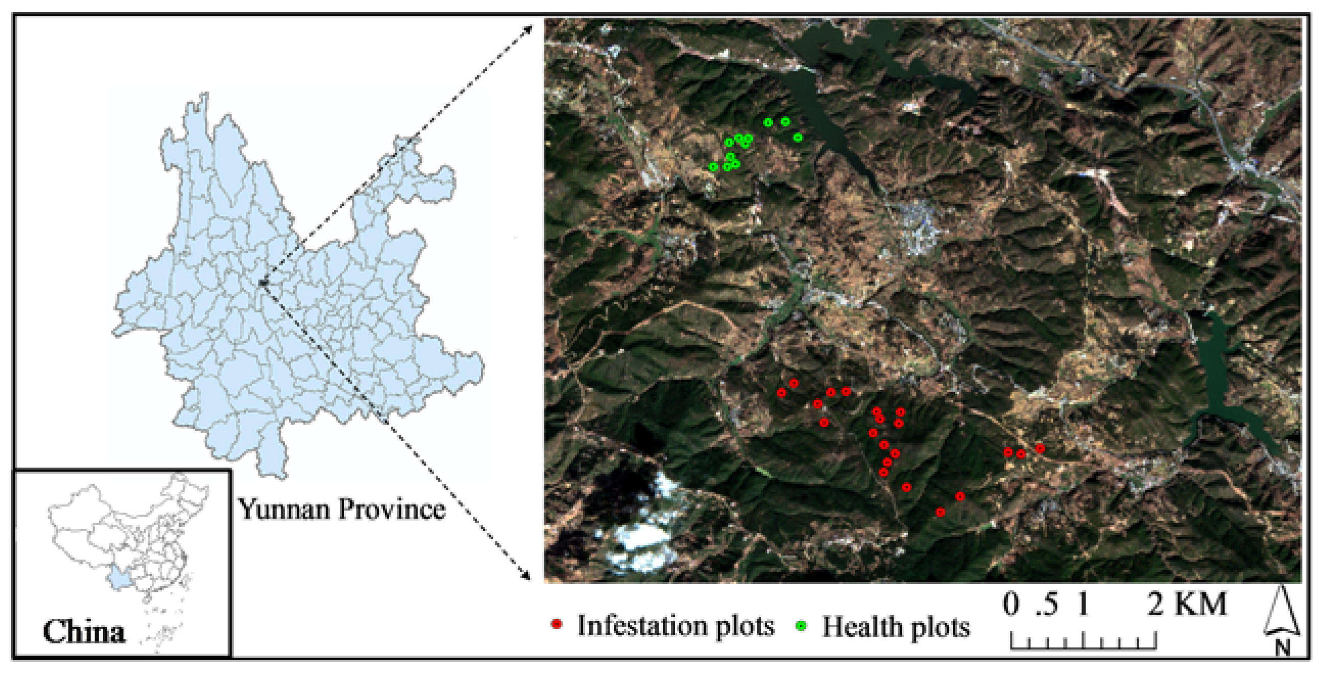
2.1. Study Site

The study site (25°14′–25°29′N, 100°48′–101°3′E), is located in the Tianfeng Mountains, Yunnan Province, in the southwest of China (Figure 1). The forest is dominated by air-sowing stands of Yunnan pine (Pinus yunnanensis Franch) with an area of about 1000 ha. Since 2010, PSB (Tomicus yunnanensis and Tomicus minor), which bore into both shoots and trunks, have been damaging the Yunnan pines, which causes serious forest dieback (approximately 50% of the forest area to date).
The field campaign was carried out from October to November in 2016. In order to cover different degrees of the damaged forest, 34 plots (30 m by 30 m), representing different levels of damage (11 healthy plots and 23 stressed plots), were set in the study area. The central GPS coordination of each plot was measured using a differential GPS device (GeoExplorer 6000, Trimble Inc., Sunnyvale, CA, USA) with an accuracy of about ±0.75 m. To quantify the tree damage, the shoots damage ratio (SDR) has been defined and measured [54]. The SDR (shown in Table 1) is the ratio of damaged shoots to total shoots of a single tree. For each tree, all damaged and healthy shoots were counted to estimate the SDR of a single tree. At each plot, we measured all trees with a diameter at breast height (DBH) greater than 4 cm. By averaging the SDR of the total of all eligible trees in a plot, the plot SDR (shown in Table 1) was calculated by:
p l o t   S D R = 1 N trees i = 1 N trees S D R i
where Ntrees is the number of trees in a plot with a DBH greater than 4 cm.

2.2. Measurements of Forest Structural Parameters

The forest structural variables were measured in each plot, including green LAI, canopy closure (CO), stem density (SD), stand average height (H), and stand average crown diameter (CD). CO was sampled in two cross-line of each plot. SD was obtained by counting the number of trees in a plot. H and CD were calculated from the average of all trees (DBH > 4 cm) within each plot. Plot green LAI was averaged using 25 evenly-spaced measurements. Each LAI measurement was conducted by a Li-Cor LAI-2200 plant canopy analyzer with a 270-degree view restrictor. Clumping is simultaneously estimated by the LAI-2200 [55,56]. In the winter season, there is a low density of understory. Summary statistics for the forest plot variables are given in Table 1.

2.3. Measurements of Needle Reflectance and Chlorophyll Content

The feeding behaviors of T. yunnanensis and T. minor are divided into two stages: (1) boring into the shoot; and (2) moving to the trunk. During the first stage, damaged shoots block the water and nutrient transfer to the needles, resulting in localized regions of chlorosis across the needle surface. In one needle, the color may vary from green to yellow. During the second stage, the “red-attack” stage, the needle color turns entirely to red. Therefore, it is interesting to measure the needle reflectance with different color combinations.
According to the common color changing sequence (green, light green, yellow, red) of pine needles, four degrees of needle damage were defined, including healthy (green), slight damage (light green), moderate damage (green-yellow, yellow), and severe damage (yellow-red, red). For each level, 50 samples were collected, sealed, and brought to an indoor laboratory. Two Avantes spectroradiometers, AvaSpec-EDU-VIS (350–850 nm), and AvaSpec-NIR1.7 (900–1700 nm) were combined to measure the needle reflectance indoors from visible (VIS) to near-infrared (NIR) bands. The spectrum resolutions were 1 nm in VIS and 3 nm in NIR, respectively. Reflectance was normalized by the sample spectrum from a white reference panel (98% diffuse reflectance). The process of the spectral measurement was conducted in a dark room. In each sample with the same degree of needle damage, about 30 to 40 number needles were tightly arranged in a grooving device with a clip because one needle is too slim to fully fill the field of view (FOV) of the optical fiber probe. For both the reflectance and transmittance measurements, the AVANTES Halogen light source (AvaLight–DHc) was used, which has a wavelength range from 400 nm to 2500 nm. Reflectance fiber with a wavelength ranging from 200 nm to 2500 nm was used, which was contacted with the needles. Transmission Dip Probes (TDP, 2 m length) were mounted on the light source and used to measure the needle transmittance. To avoid external light interference, the optical fiber probe with a FOV of 25° was installed in a reflection probe holder (RPH-1, https://www.avantes.com/products/fiber-optics/item/260-reflection-probe-holders). The fiber probe holder was attached to the sample grooving device to measure the needle spectra. Each sample (from the tip to base of the needles) was measured five times and averaged to minimize instrument noise.
Correspondingly, the LCC of the needles were measured using the Chlorophyll Content Meter (CCM-300, Opti-Science, Inc., Hudson, NH, USA) based on the fluorescence ratio of red emissions measured at 700 nm and 735 nm. The chlorophyll (Chl) content was calculated using the equation [Chl] = 634F735/F700 + 391 [57]. There was a linear response to Chl content ranging from 41–675 mg m−2, with a determination coefficient of R2 greater than 0.95. The CCM-300 was capable of conducting nondestructive measurement of the chlorophyll of tiny leaves (such as needles) with a leaf clip holder. The CCM-300 was calibrated (R2 = 0.94) using 28 independent samples measured by a standard UV-2600 Spectrophotometer and using 95% anhydrous ethanol as dissolving reagent [58].
For each sample, three sections of the tip, center, and base of the needles were measured to calculate the average LCC. The results of the LCC are shown in Table 2.
Similar to the needle scale, the infested shoots are also divided into healthy, slight, moderate and severe levels of damage (Figure 2). The severity of damage to individual shoots was visually estimated: (a) healthy, for shoots with green needles and no insect attack; (b) light, for shoots with a boring attack and consisting of light or yellowish needles; (c) moderate, with half yellow needles; and (d) severe, for shoots with almost completely red needles. The mean LCC of the four classes of needles was used to determine the LCC of a single shoot. For each class of shoots, 50 shoot samples with varied needle density and length were chosen to calculate the mean LCC of the shoots, which was then defined as the shoot LCC (LCCshoot). The statistics of LCCshoot are shown in Table 2.
It is difficult to determine the average LCC for a stressed tree or plot. Traditionally, the total plot LCC is a multiplied value of a mean LCC and LAI [59,60]. This method is easy and quick for estimating the total plot LCC when the canopy leaves are relatively homogenous. However, our key question is around how to determine the mean LCC for a heterogeneous canopy. For Yunnan pines, the trees may have different degrees and numbers of needles or shoots. The heterogeneous crowns lead to difficulty in determining the mean LCC through random sampling of needles or shoots. In this paper, the LCC of a single tree (LCCtree) is calculated with a weighted average method:
L C C tree = L C C shoot , healthy n shoot , healty + L C C shoot , slight n shoot , slight + L C C shoot , moderate n shoot , moderate + L C C shoot , severe n shoot , severe N shoots
where LCCshoot,healthy, LCCshoot,slight, LCCshoot,moderate, and LCCshoot,severe are the mean chlorophyll content of the healthy, slight, moderate, and severely damaged shoots, respectively. Nshoots is the total number of shoots of a single tree.
Then, the average LCC of a plot with Ntrees trees, the LCCplot (see Table 1), is as follows:
L C C plot = 1 N trees i = 1 N trees L C C tree , i

2.4. Sentinel 2A Images and Processing

The Sentinel-2 (S2) satellite features a Multi-Spectral Instrument (MSI) with a 290 km field of view (FOV). This MSI provides 13 spectral bands, ranging from the visible and near-infrared (VNIR) to the short-wave infrared (SWIR), with four bands (B2–B4, B8) at 10 m spatial resolution, six bands (B5–B7, B8a, B11, B12) at 20 m spatial resolution, and three bands (B1, B9, B10) at 60 m spatial resolution [61]. The high spatial resolution, wide FOV, and broad spectral coverage of S2 are designed to map land use and land cover (LULC), as well as change detection, geophysical variables (i.e., LCC, LAI) mapping, and risk, such as forest insect detection. S2 imagery has a high quality of geometry and radiation [62]. The Level 1C product is geo-coded with a sub-pixel registration accuracy for users and provides the top of the atmosphere (TOA) reflectance [62]. Images collected on 31 December 2016 (Relative Orbit number: R104) were used in this paper, taken at a time that was almost cloud-free (cloud cover less 1%). The atmosphere correction was conducted using the SEN2COR (http://step.esa.int/main/third-party-plu-gins-2/sen2cor/) tools. We used the bands from B2 to B8a, which are highly sensitive to chlorophyll and LAI variations. The bands at a spatial resolution of 10 m were aggregated to 20 m, resulting in eight bands in VNIR at 20 m.

2.5. The Needle-Reflectance Model LIBERTY

The LIBERTY model was developed to describe the spectral properties of conifer needles [44]. The model employs nine biophysical/biochemical parameters (Table 3) to simulate needle reflectance and transmittance in the VNIR and SWIR wavelengths (400–2500 nm) at 5 nm intervals. The model linearly sums in vivo specific absorption coefficients, scaled by their respective concentrations, to calculate a global absorption coefficient [63]. The global absorption coefficient, in conjunction with the structural parameters of average cell diameter (d), intercellular air gap (xu), and needle thickness (t), were used to calculate needle reflectance and transmittance.

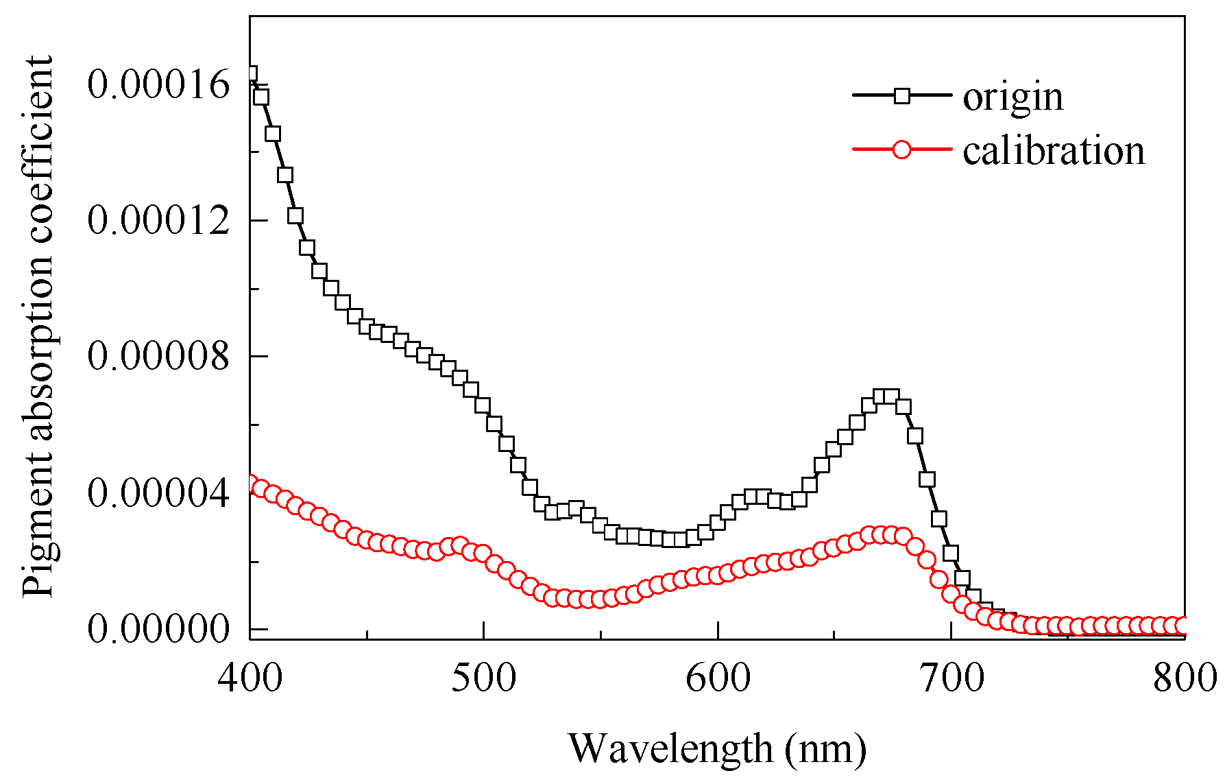
2.5.1. Calibration of Pigment Absorption Coefficients

The LIBERTY model in vivo specific absorption coefficients were measured from jack pine needles during the Boreal Ecosystem Atmosphere Study (BOREAS) campaign [44]. The leaf model (e.g., PROSPECT/LIBERTY) physically describes the relationship between biochemical/structure parameters and spectral reflectance; thus, it is expected to be independent of species and site conditions. However, the specific absorption coefficients of pigment in different species are not completely consistent. Many studies indicated that better accuracy of leaf/needle optical properties and biochemical parameters were estimated after being validated and calibrated with real measurement of leaf/needle reflectance [44,45,63,64,65,66,67,68]. Yunnan pine is a different species to jack pine, thus, the LIBERTY model needs to be calibrated before it can accurately simulate vegetation reflectance spectra at the local scale and inversed to estimate leaf biochemical parameters [64,65]. In order to accurately model needle reflectance, calibration of pigment absorption coefficients should be considered. The Newton–Raphson iterative method was applied to calibrate the LIBERTY model [63] using a randomly selected 40% of healthy needles from field measurements for model calibration. The remainder were used for model validation. The validation accuracy was assessed by the mean relative error (MRE) between the modeled and measured needle reflectance.

2.5.2. Simulation of Heterogeneous Leaf Reflectance

Insect damage can cause heterogeneous leaves with patchy chlorosis which strongly influences the whole leaf reflectance because of the non-uniform distribution of chlorophyll [48]. According to the BARTON study [48], a heterogeneous leaf area was split into two regions with distinct chlorophyll concentrations: (1) the damaged region with the fraction of leaf (f) and chlorophyll concentration Cα; and (2) the healthy region (1 − f) with chlorophyll concentration Cβ. The mean leaf chlorophyll concentration Cmean is
C mean = f   C α + ( 1 f ) C β
Assuming that Cα = 0 for the chlorophyll content of the dead leaf area, and f is the dead leaf area fraction, Equation (4) is simplified as
C mean = ( 1 f ) C β
Because f represents the degree of needle damage, we use it as a damage indicator called the “Yellow Index” (YI) [69]. Therefore, Equation (5) can be converted into a new form (Cmean = (1 − YI)Cβ), in which Cβ refers to the chlorophyll content of the healthy region for a heterogeneous needle.
Assuming that two regions of a heterogeneous leaf are scattered or absorbed without interaction, the reflectance Rλ,Cmean is linearly mixed [48] between the dead region reflectance Rλ,=0 and the healthy region reflectance Rλ,:
R λ , C mean = YI   R λ , C α = 0 + ( 1 YI ) R λ , C β
Similarly, the mixed transmittance of a heterogeneous leaf Tλ,Cmean is as follows:
T λ , C mean = YI   T λ , C α = 0 + ( 1 YI ) T λ , C β
where Tλ,Cα=0 and Tλ,Cβ are the transmittance of the dead region and healthy region, respectively. The healthy needle spectra (Rλ,, Tλ,) can be effectively simulated by the LIBERTY model following calibration with healthy needles. However, under stress conditions, the LIBERTY model performs bad and should be modified to achieve better accuracy [69]. The reason for this is that the LIBERTY model only considers a single pigment absorption coefficient for chlorophyll and carotenoid instead of separating them into individual pigments [44,70]. In fact, chlorosis results from the interaction of multiple pigments of the leaf. Pigments such as carotenoid, brown, and anthocyanins, in particular, cause a yellow or red leaf [71]. To overcome this limitation of LIBERTY, YI was used as a corrected fraction to describe the effect of the mixture of multiple pigments correlated with chlorosis on needle reflectance. In the process of the needle reflectance simulation, YI was independent of the radiative transfer modeling equation of LIBERTY. The measured spectra of red needles (LCC = 0 mg m−2) of Yunnan pine was used as the prior-knowledge of the dead needle spectra (Rλ,=0, Tλ,=0); it can be replaced by a generally dead or senescent leaf spectra.
For convenience, the original, calibrated (including the calibrated pigment absorption coefficient), and modified (includes the calibrated pigment absorption coefficient and YI) LIBERTY models are named LIBERTY0, LIBERTY1, and LIBERTY2, respectively. The performance of the infested needle reflectance simulation was evaluated using the mean relative error (MRE) based on measured and simulated needle reflectance.
As described above, there are four levels of LCC: needle, shoot, single tree, and plot. SDR is this concept at the tree level. At the plot scale, the mean SDR of all trees is used to represent the degree of damage. Therefore, the plot LCC is a combined value of three scales (tree, shoot, and needle):
L C C plot = 1 N trees i = 1 N trees ( L C C shoot , healthy ( 1 S D R i ) + L C C shoot , damaged S D R i )
L C C plot = 1 N trees N shoots i = 1 N trees j = 1 N shoots ( L C C needle , healthy ( 1 YI j ) + L C C needle , damaged YI j )
where LCCshoot,healthy, LCCshoot,damaged, LCCneedle,healthy, and LCCneedle,damaged are the mean LCC of the healthy and damaged shoots or needles.
Assuming that all trees in a plot have the same degree of damage and needles or shoots are randomly distributed in the tree crowns with either healthy or dead properties, Equations (8)–(9) can be derived as
L C C plot = L C C shoot , healthy ( 1 plot   S D R )
L C C plot = L C C needle , healthy ( 1 YI )
Based on the assumption above, LCCshoot,healthy is equal to LCCneedle,healthy. Although YI is defined at the needle scale, by assuming that needles are randomly distributed, YI is numerically equal to the plot SDR.

2.6. INFORM Model

The INFORM model [36], coupled with LIBERTY0, LIBERTY1, and LIBERTY2, is used to simulate the bidirectional reflectance (BRF) of forest stands between 400 and 2500 nm. The main input parameters of the INFORM model are shown in Table 3.

2.7. Look-Up-Table (LUT) Inversion

LUT is a simple but effective strategy for remote sensing inversion, which can help to alleviate the drawback of the ill-posed problem [72]. The LUT inversion can be divided into two steps: (1) The generation of LUT by RTM; and (2) the selection of the solution corresponding to the given measurement. LUT consists of input parameter combinations and the associated output simulation of canopy reflectance. For the generation of LUT, the range and distribution of the LIBERTY and INFORM model parameters should be defined. Table 3 shows the ranges (minimum, maximum, and a step) of the leaf and canopy variables. The minimum and maximum of single tree LAIs (LAIs = LAI/CO), understory LAI (LAIu), LCC, H, CD, SD, thee hotspot parameter (hot), and the diffuse light fraction (skly) are defined based on prior knowledge from field measurements and other similar studies [47]. According to the sensitivity analysis of LIBERTY [44,63,64], water, lignin/cellulose, and protein contribute mostly in NIR with wavelengths greater than 1000 nm [44,63]. Therefore, the water content (CW), lignin and cellulose content (CL), and nitrogen content (CP) were held constant. Sun and viewing conditions correspond to the situation of the satellite overpass. A LUT length of 100,000 cases of parameter combinations was chosen using uniform random sampling in accordance with previous research [73,74]. This LUT size proved to be feasible and a larger LUT size may not influence the estimation accuracy according to similar research [55,56,72]. Subsequently, the coupled models LIBERTY0-INFORM, LIBERTY1-INFORM, and LIBERTY2-INFORM were applied to simulate canopy reflectance (ρcanopy) using the 100,000 cases of parameter combinations. The simulated canopy reflectance with 5 nm intervals was re-sampled to the eight bands of S2A using S2 MSI spectral response functions (SRF) (https://earth.esa.int/web/sentinel/document-library/content/-/article/sentinel-2a-spectral-responses) with the following form [75]:
ρ image ( λ ) = λ max λ max ρ canopy ( λ o ) f ( λ o )   d λ o λ max λ max f ( λ o )   d λ o
where ρimage (λ) refers to the broadband reflectance of S2A for given band λ, f(λo) refers to the SRF of the corresponding wavelength, and λmax and λmin refer to the upper and lower limit of each band interval, respectively. Finally, the input parameter combinations and associated output simulation of canopy reflectance were stored in LUT.
In the S2A imagery, we used the average reflectance of 3 × 3 pixels around the plot location to reduce the uncertainty of location error due to the inconsistency between plot dimensions (30 m) and the S2A pixel resolution (20 m). The relative error (RE) (see Table 4) between the average reflectance of 3 × 3 pixel reflectance and plot location pixel reflectance was used to explore pixel variation. Table 4 shows that the difference between the plot location pixel and 3 × 3 pixels was small, at 4.49% of the mean RE. The average reflectance of 3 × 3 pixels can represent the measured reflectance of each plot.
Table 5 shows the 12 different potentially promising cost functions (CFs) for LUT inversion from three broad families (information measures, M-estimates, and the minimum contrast method) [76]. As demonstrated by Rivera [55], these CFs should be competed with one another to find the best inversion solution. The competition is based on D [P, Q], the distance between two functions, where P = ( p ( λ 1 ) , , p ( λ n ) ) is the reflectance of satellite data; Q = ( q ( λ 1 ) , , q ( λ n ) ) is the LUT simulated reflectance; and λ1, …, λn represent the n spectral bands.
Other than the optimization of cost functions, two regularization options are also applied in LUT-based inversion strategies to further optimize the robustness of the estimates [55,56]. First, a series of Gaussian white noise, from 0–20% with a step 1%, was added to LUT simulate canopy reflectance to account for uncertainties attached to the models and measurements [55,56,73,77]. Second, multiple best solutions were used instead of a single best solution to calculate the estimated values [55,56,73,78]. Several studies have demonstrated that the single best parameter combination corresponding to the smallest distance calculated by a cost function (e.g., RMSE) does not necessarily lead to the best accuracies [43,78]. Different optimization numbers and the mutual effect on these regularization options have been systematically assessed in previous studies [55,56].
The inversed LCC and LAI values were validated using field measurements. The accuracy was assessed by R2, the index of agreement (IOA) [79] (IOA is a standardized measure of the degree of model prediction error and varies between 0 and 1), root mean square error (RMSE) and the normalized RMSE (NRMSE) [72]. The inversion performance of INFORM using three versions of LIBERTY models was evaluated by calculating the deviations between the retrieved values and measured values through RMSE and NRMSE. The NRMSE was used to determine the best CFs and optimal regularization options.

3. Results

3.1. Pigment Absorption Coefficient Calibration and Needle Reflectance Simulation

Figure 3 shows the pigment absorption coefficient of the original and calibrated LIBERTY models using the measured needle spectral. It is clear that the values of the calibrated pigment absorption coefficient are lower than the original values in most of the wavelengths. By increasing the YI from 0 to 1 with a fixed chlorophyll content of the healthy region (Cβ) of 400 mg m−2, the corresponding heterogeneous needle reflectance (Figure 4a) was simulated by LIBERTY2. The first derivative is also presented in Figure 4b. From Figure 4, we can see the effect of the chlorotic area fraction on needle reflectance:
(a)
The needle reflectance decreases significantly in green and NIR bands but increases in the red band in response to the increase of the YI (Figure 4a).
(b)
In the first derivative of the heterogeneity of needle reflectance, the red shift in the green peak and blue shift in the red valley are visible due to the damage of pest stress (Figure 4b).
(c)
A slight change in the red edge position (710 nm) is found (Figure 4b).
Figure 5 shows the reflectance simulations using LIBERTY0, LIBERTY1, and LIBERTY2 for different severities of damaged needles. The LIBERTY1 model performs better than the LIBERTY0 model when simulating healthy, slightly, and moderately damaged needle reflectance within 400–800 nm. The better performance of LIBERTY1 over LIBERTY0 in modeling needle reflectance indicates that calibration of the pigment absorption coefficient improved the accuracy. Both the LIBERTY0 and LIBERTY1 models failed in reflectance simulation of severely damage needles; while LIBERTY2 effectively simulated needles with all levels of damage. The result of validation data shows that the accuracy of reflectance simulation has an MRE between 18.1% and 72% for LIBERTY0, between 2.88% and 71.8% for LIBERTY2, and between 1.4% and 18% for LIBERTY2. This result indicates that the linear mixing method is robust in damaged needle reflectance simulation. Furthermore, for each sample of needles, we can obtain the best-simulated reflectance and corresponding YI when inverting LIBERTY2. The result shows that the derived YI (healthy: 0 < YI < 0.1, slight: 0.05 < YI < 0.15, moderate: 0.15 < YI < 0.5, severe: 0.5 < YI < 1) can be used to separate the different degrees of needle damage from the leaf reflectance spectra. If using YI values, the moderate to severe degrees of damage can be distinctly separated from healthy needles or those with a slight degree of damage. However, using the YI, it is still difficult to detect the difference between healthy and slight degrees of damage in the range of 0.05 < YI < 0.1, when the needle damage is too weak.

3.2. Leaf Chlorophyll Content (LCC) and Leaf Area Index (LAI) Retrieval

Based on the LUT strategy and two regularization options, the performances of LCC and LAI retrieval are presented in Figure 6 using the INFORM model coupled with LIBERTY0, LIBERTY1, and LIBERTY2, respectively. Figure 6 shows the accuracies of LCC and LAI retrieval using different CFs and regularization options. It can be seen that different models may achieve the best retrieval with different CFs, which can be explained by different CFs dealing with different types of error distributions [56]. For example, the best CFs are L-divergence for LIBERTY0-INFORM (at 8% multiple solutions and 6% noise), normal distribution-LSE for LIBERTY1-INFORM (at 3% multiple solutions and 5% noise) and least absolute error for LIBERTY2-INFORM (at 1% multiple solutions and 2% noise). The accuracy of LCC retrieval by LIBERTY1-INFORM (R2 = 0.44, RMSE = 58.87 mg m−2, NRMSE = 26.40% and IOA = 0.65) is higher than that of LIBERTY0-INFORM (R2 = 0.34, RMSE = 76.44 mg m−2, NRMSE = 34.23% and IOA = 0.57). The better performance of LIBERTY1-INFORM on LCC retrieval confirms that calibration improved the estimation accuracy. LIBERTY2-INFORM has the highest accuracy (R2 = 0.49, RMSE = 56.24 mg m−2, NRMSE = 25.22% and IOA = 0.72) in LCC retrieval. However, inversed LCC was systematically underestimated above 300 mg m−2, while being overestimated below 300 mg m−2.
Similar to LCC retrieval performance, LIBERTY2-INFORM produced better accuracy of LAI (R2 = 0.73, RMSE = 0.17 m m−2, NRMSE = 11.41% and IOA = 0.91) than LIBERTY0-INFORM (R2 = 0.38, RMSE = 0.43 m m−2, NRMSE = 28.85% and IOA = 0.68) and LIBERTY1-INFORM (R2 = 0.63, RMSE = 0.23 m m−2, NRMSE = 15.44% and IOA = 0.86). However, the NRMSE of LAI retrieval is lower than that of LCC.

3.3. Estimation of Plot Shoots Damage Ratio (SDR)

Based on the above results, the LIBERTY2-INFORM model was used to create LUT and inverse LCC, LAI, plot SDR and YI over the 34 plots. The inversed YI is positively related to plot SDR (Figure 7), and the R2 was 0.40 and the RMSE was 0.15.

4. Discussion

4.1. The Contribution of Heterogeneous Leaf Reflectance Simulation

In this paper, three different versions of LIBERTY (LIBERTY0, LIBERTY1, and LIBERTY2) were used to model the reflectance of heterogeneous needles. LIBERTY1 performed better than LIBERTY0 (shown in Figure 5) in simulating needle reflectance for needles were healthy to moderately degree damaged. This result confirmed that calibration of the pigment absorption coefficient could help improve the accuracy of modeling needle reflectance, which was consistent with previous research [64]. However, both LIBERTY0 and LIBERTY1 were out-performed for modeling the reflectance of severely damaged needles. There were two major reasons for this: (1) the absorption coefficient was constant in this study, whereas, in reality, the mix of light-absorbing pigments might change in response to declining LCC or localized chlorosis [48]; and (2) a single pigment did not quantify individual pigments, which provide specific services (such as giving leaves their yellow or red color) to leaves and absorb different amounts of radiation [65,70]. Depending on the cause of chlorosis, there may be concurrent change to multiple pigments such as carotenoids and anthocyanin that would alter reflectance. However, the LIBERTY model only considers a total single pigment instead of separating it into specific individual pigments. Additionally, LIBERTY did not consider the anthocyanins, which were closely associated with the color of the needles [71]. Therefore, LIBERTY0 and LIBERTY1 could not accurately model the reflectance of yellow or red needles.
In this study, the spectral linear mixing method was used to describe the effect of other pigments which were correlated with chlorosis on needle reflectance. Thus, LIBERTY2 improved the simulation of reflectance accuracy for damaged needles. The spectral linear method was a semi-empirical method, it cannot depict the mix of light-absorbing multiple pigments in response to certain forms of stress from a radiative transfer modeling equation. Further, cell structure parameters such as cell diameter (D) and intercellular airspace (xu) would decrease during the beetle attack [27,80]. Because the LIBERTY model requires prior knowledge of D and xu to invert reflectance values [63], accurate cell structure values might improve the accuracy of modeling the reflectance of damaged needles.

4.2. LCC, LAI, and Plot Shoots Damage Ratio Estimation (SDR) Performance

The inversion accuracies of LCC, LAI, and plot SDR were used to compare the capabilities of INFORM coupled with three versions of the LIBERTY model. The LIBERTY2-INFORM has the best accuracy. These results indicate that accurate leaf-scale RT can improve the parameter retrieval performance of the canopy model [64]. The good performance of LAI retrieval is because INFORM effectively considers the sparse canopy structure, understory vegetation, and shadow components [81]. However, the performance of LCC retrieval was worse, although the non-uniform distribution of the chlorophyll impact canopy reflectance has been considered. At the plot scale, LAI can be measured using a suitable optical instrument (e.g., LAI-2000/2200). However, there are no direct approaches or instruments to measure the LCC of a forest plot. Instead, the random sampling method is used to estimate the average value and represent the mean LCC of the plot. The sampling error led to uncertainty in the LCC inversion. In this study, the accuracy of the LCC of the plot depended on the correct classification of the shoot damage class. A more exhaustive classification of shoot damage may improve LCC inversion accuracy.
As for the RT model, 1-dimensional (1D) models are commonly suited to a relatively uniform canopy with a vertical variation of structure but very limited in depicting the complex variation of chlorophyll content in the horizontal structure. INFORM is an extended 1D model, which uses the crown diameter and stem density to describe the horizontal variation of the forest canopy. However, the canopy reflectance simulation was very sensitive to the variations of crown diameter according to the sensitivity analysis of FLIM [82], which added to the inversion error. Hence, the inversion accuracy of LCC is difficult to improve in 1D models. In the future, we will consider using a 3-dimensional (3D) canopy model which can rapidly simulate (e.g., RAPID [83]), to allow the defined 3D scene to invert LCC in PSB stress.
A new index, the YI, can be inversed simultaneously with LCC and LAI. This index theoretically equals plot SDR, which is also evaluated in Figure 7 (R2 = 0.40). An unexpected result is the systematic underestimation of YI in damaged plots (plot SDR > 0.2). This may be caused by two major factors: (1) the effect of the clumping of needles or shoots on canopy reflectance; and (2) the overestimation of field SDR because the shoot counting is empirical. As long as a shoot has several yellow needles, it will be counted as a damaged shoot. Conversely, YI is non-zero in healthy plots (plot SDR = 0). This can be explained by the underestimation of LCC (LCC > 300 mg m−2) by LIBERTY2-INFORM, influenced by the green understory. The green understory will strongly impact YI effectiveness in the accuracy of predicting plot SDR because of the contribution of the understory to the forest reflectance in a sparse canopy. Therefore, the YI will be more effective in a dense canopy with at least slight damage. Furthermore, the spatial arrangement of damaged needles is another important impact factor. For Yunnan pine, the stressed canopy reflectance is distinctly different from that of a healthy canopy when the damaged needles are at the top part of the crown. In that case, plot SDR can be effectively estimated by the YI. However, when the damaged needles are on the bottom (understory) part of the crown, stressed canopy reflectance is similar with healthy (or slight damage) canopy reflectance because the damaged needles are blocked by healthy needles in a given observation direction. The plot SDR will, therefore, be seriously underestimated when damaged needles are on the bottom (understory) of the crown. A 3D canopy model will be considered in the future to simulate the spatial arrangement of the damaged needles/shoots.

4.3. Role of LUT Setting

In this paper, we used a uniform distribution and fixed ranges to create LUT for both LCC and LAI. However, this setting influences the accuracy of LCC, LAI and the plot SDR estimation. For example, it may cause an error in the variable estimation if the definition of the parameters is too broad compared to the measurements [84]. Because of the external disturbance factors (e.g., pest and pollution), there are difficulties in determining the suitable distribution of parameters. LCC and LAI have different effects on different wavelength regions. LCC takes the dominant role in the visible region; while LAI variations cause spectral variation over the whole VNIR [85,86]. As a result, the band from B2 to B5 are enough to achieve a good LCC retrieval performance; and adding bands may introduce errors. As for LAI, adding bands logically improved the inversion performance [55,56].

5. Conclusions

In this study, the spectral linear mixing method was used in LIBERTY2 which improved the accuracy of modeling heterogeneous needle reflectance. The coupled model LIBERTY2-INFORM was used to quantitatively assess PSB stress in Yunnan pine forests. The YI was introduced in the RT to predict plot SDR representing PSB stress. The YI was used to model the non-uniform distribution of chlorophyll within the needles. The results show significant improvement of needle reflectance simulation under severe damage conditions. Inversion of INFORM-LIBERTY2 using the LUT inversion method leads to the best LAI (R2 = 0.73, RMSE = 0.17 m m−2, NRMSE = 11.41% and IOA = 0.92) and LCC (R2 = 0.49, RMSE = 56.24 mg m−2, NRMSE = 25.22% and IOA = 0.72) retrieval performance for Yunnan pine forests under PSB stress.
Our study implies that a more accurate simulation of leaf optical properties can help enhance the performance of biophysical parameters inversion. The YI is a simple and potential indicator to estimate plot SDR in order to assess PSB outbreaks. To improve the inversion accuracy of the YI, LCC, and LAI, a 3D RT model will be used in the next study.

Author Contributions

Q.L., L.Y., and H.H. conceived and designed the experiments; Q.L., L.Y., and J.W. conducted the field experiments; L.Y. and H.H. analyzed the data; Q.L. and H.H. wrote the paper.

Funding

This paper has been supported by the Chinese Natural Science Foundation Project (41571332).

Acknowledgments

Thanks Clement Atzberger for providing the INFORM code.

Conflicts of Interest

The authors declare no conflict of interest.

References

  1. Sedjo, R.A. The carbon cycle and global forest ecosystem. Water Air Soil Pollut. 1993, 70, 295–307. [Google Scholar] [CrossRef]
  2. Schlamadinger, B.; Marland, G. The role of forest and bioenergy strategies in the global carbon cycle. Biomass Bioenergy 1996, 11, 275–300. [Google Scholar] [CrossRef]
  3. Waring, R.H.; Pitman, G.B. Modifying Lodgepole Pine Stands to Change Susceptibility to Mountain Pine Beetle Attack. Ecology 1985, 66, 889–897. [Google Scholar] [CrossRef]
  4. Lewis, S.L.; Edwards, D.P.; Galbraith, D. Increasing human dominance of tropical forests. Science 2015, 349, 827–832. [Google Scholar] [CrossRef] [PubMed] [Green Version]
  5. Nelson, R.F. Detecting forest canopy change due to insect activity using Landsat MSS. Photogramm. Eng. Remote Sens. 1983, 49, 1303–1314. [Google Scholar]
  6. Rock, B.N.; Vogelmann, J.E.; Williams, D.L.; Vogelmann, A.F.; Hoshizaki, T. Remote Detection of Forest Damage. Bioscience 1986, 36, 439–445. [Google Scholar] [CrossRef]
  7. Jan, V.; Andrew, R.; Christine, S.; Darius, C. Forecasting tree mortality using change metrics derived from MODIS satellite data. Forest Ecol. Manag. 2009, 258, 1166–1173. [Google Scholar]
  8. Wolter, P.T.; Townsend, P.A.; Sturtevant, B.R. Estimation of forest structural parameters using 5 and 10 meter SPOT-5 satellite data. Remote Sens. Environ. 2009, 113, 2019–2036. [Google Scholar] [CrossRef]
  9. Babst, F.; Esper, J.; Parlow, E. Landsat TM/ETM+ and tree-ring based assessment of spatiotemporal patterns of the autumnal moth (Epirrita autumnata) in northernmost Fennoscandia. Remote Sens. Environ. 2010, 114, 637–646. [Google Scholar] [CrossRef]
  10. Walter, J.A.; Platt, R.V. Multi-temporal analysis reveals that predictors of mountain pine beetle infestation change during outbreak cycles. Forest Ecol. Manag. 2013, 302, 308–318. [Google Scholar] [CrossRef]
  11. Fassnacht, F.E.; Latifi, H.; Ghosh, A.; Joshi, P.K.; Koch, B. Assessing the potential of hyperspectral imagery to map bark beetle-induced tree mortality. Remote Sens. Environ. 2014, 140, 533–548. [Google Scholar] [CrossRef]
  12. Rullán-Silva, C.; Olthoff, A.E.; Pando, V.; Pajares, J.A.; Delgado, J.A. Remote monitoring of defoliation by the beech leaf-mining weevil Rhynchaenus fagi in northern Spain. Forest Ecol. Manag. 2015, 347, 200–208. [Google Scholar] [CrossRef]
  13. Baker, E.H.; Painter, T.H.; Schneider, D.; Meddens, A.J.H.; Hicke, J.A.; Molotch, N.P. Quantifying insect-related forest mortality with the remote sensing of snow. Remote Sens. Environ. 2017, 188, 26–36. [Google Scholar] [CrossRef]
  14. Senf, C.; Pflugmacher, D.; Wulder, M.A.; Hostert, P. Characterizing spectral–temporal patterns of defoliator and bark beetle disturbances using Landsat time series. Remote Sens. Environ. 2015, 170, 166–177. [Google Scholar] [CrossRef]
  15. Meigs, G.W.; Kennedy, R.E.; Cohen, W.B. A Landsat time series approach to characterize bark beetle and defoliator impacts on tree mortality and surface fuels in conifer forests. Remote Sens. Environ. 2011, 115, 3707–3718. [Google Scholar] [CrossRef]
  16. Niemann, K.O.; Quinn, G.; Stephen, R.; Visintini, F.; Parton, D. Hyperspectral Remote Sensing of Mountain Pine Beetle with an Emphasis on Previsual Assessment. Can. J. Remote Sens. 2015, 41, 191–202. [Google Scholar] [CrossRef]
  17. Wulder, M.A.; Dymond, C.C.; White, J.C.; Leckie, D.G.; Carroll, A.L. Surveying mountain pine beetle damage of forests: A review of remote sensing opportunities. Forest Ecol. Manag. 2006, 221, 27–41. [Google Scholar] [CrossRef]
  18. Peterman, W.; Waring, R.H. Does overshoot in leaf development of ponderosa pine in wet years leads to bark beetle outbreaks on fine-textured soils in drier years? Forest Ecosyst. 2014, 1, 24. [Google Scholar] [CrossRef]
  19. Chen, G.; Meentemeyer, R.K. Remote Sensing of Forest Damage by Diseases and Insects. In Remote Sensing for Sustainability; CRC Press: Boca Raton, FL, USA, 2016; pp. 145–162. [Google Scholar]
  20. Coops, N.C.; Johnson, M.; Wulder, M.A.; White, J.C. Assessment of QuickBird high spatial resolution imagery to detect red attack damage due to mountain pine beetle infestation. Remote Sens. Environ. 2006, 103, 67–80. [Google Scholar] [CrossRef]
  21. Olsson, P.O.; Jönsson, A.M.; Eklundh, L. A new invasive insect in Sweden—Physokermes inopinatus: Tracing forest damage with satellite based remote sensing. Forest Ecol. Manag. 2012, 285, 29–37. [Google Scholar] [CrossRef]
  22. Goodwin, N.R.; Coops, N.C.; Wulder, M.A.; Gillanders, S.; Schroeder, T.A.; Nelson, T. Estimation of insect infestation dynamics using a temporal sequence of Landsat data. Remote Sens. Environ. 2008, 112, 3680–3689. [Google Scholar] [CrossRef]
  23. Nicholasc, C.; Steven, G.; Michaela, W.; Sarahe, G.; Trisalyn, N.; Nicholasr, G. Assessing changes in forest fragmentation following infestation using time series Landsat imagery. Forest Ecol. Manag. 2010, 259, 2355–2365. [Google Scholar]
  24. Coops, N.C.; Wulder, M.A.; Iwanicka, D. Large area monitoring with a MODIS-based Disturbance Index (DI) sensitive to annual and seasonal variations. Remote Sens. Environ. 2009, 113, 1250–1261. [Google Scholar] [CrossRef]
  25. Skakun, R.S.; Wulder, M.A.; Franklin, S.E. Sensitivity of the thematic mapper enhanced wetness difference index to detect mountain pine beetle red-attack damage. Remote Sens. Environ. 2003, 86, 433–443. [Google Scholar] [CrossRef]
  26. Wah, L.O.; Chong, P.C.J.; Li, B.; Asundi, A.K. Signature Optical Cues: Emerging Technologies for Monitoring Plant Health. Sensors 2008, 8, 3205. [Google Scholar]
  27. AHERN, F.J. The effects of bark beetle stress on the foliar spectral reflectance of lodgepole pine. Int. J. Remote Sens. 1988, 9, 1451–1468. [Google Scholar] [CrossRef]
  28. Shiklomanov, A.N.; Dietze, M.C.; Viskari, T.; Townsend, P.A.; Serbin, S.P. Quantifying the influences of spectral resolution on uncertainty in leaf trait estimates through a Bayesian approach to RTM inversion. Remote Sens. Environ. 2016, 183, 226–238. [Google Scholar] [CrossRef]
  29. Liang, S. Quantitative Remote Sensing of Land Surfaces; Wiley-Interscience: Hoboken, NJ, USA, 2004; pp. 413–415. [Google Scholar]
  30. Li, X.W.; Wang, J.D. Optical Remote Sensing Model and Parameterization for Vegetation; Science Press: Beijing, China, 1995. [Google Scholar]
  31. Verhoef, W. Light scattering by leaf layers with application to canopy reflectance modeling: The SAIL model. Remote Sens. Environ. 1984, 16, 125–141. [Google Scholar] [CrossRef] [Green Version]
  32. Leblanc, S.G.; Bicheron, P.; Chen, J.M.; Leroy, M.; Cihlar, J. Investigation of directional reflectance in boreal forests with an improved four-scale model and airborne POLDER data. IEEE Trans. Geosci. Remote Sens. 1999, 37, 1396–1414. [Google Scholar] [CrossRef]
  33. Chen, J.M.; Li, X.; Nilson, T.; Strahler, A. Recent advances in geometrical optical modelling and its applications. Remote Sens. Rev. 2000, 18, 227–262. [Google Scholar] [CrossRef]
  34. Li, X.; Strahler, A.H. Geometric-Optical Bidirectional Reflectance Modeling of a Conifer Forest Canopy. IEEE Trans. Geosci. Remote Sens. 1986, GE-24, 906–919. [Google Scholar] [CrossRef]
  35. Atzberger, C. Development of an invertible forest reflectance model: The INFOR-model. In A Decade of Trans-European Remote Sensing Cooperation, Proceedings of the 20th EARSeL Symposium, Dresden, Germany, 14–16 June 2000; Buchroithner, M., Ed.; CRC Press: Boca Raton, FL, USA, 2000. [Google Scholar]
  36. Schlerf, M.; Atzberger, C. Inversion of a forest reflectance model to estimate structural canopy variables from hyperspectral remote sensing data. Remote Sens. Environ. 2006, 99, 281–294. [Google Scholar] [CrossRef]
  37. Li, X.; Strahler, A.H.; Woodcock, C.E. A hybrid geometric optical-radiative transfer approach for modeling albedo and directional reflectance of discontinuous canopies. IEEE Trans. Geosci. Remote Sens. 1995, 33, 466–480. [Google Scholar]
  38. Gastellu-Etchegorry, J.P.; Demarez, V.; Pinel, V.; Zagolski, F. Modeling radiative transfer in heterogeneous 3-D vegetation canopies. Remote Sens. Environ. 1996, 58, 131–156. [Google Scholar] [CrossRef]
  39. Borel, C.C.; Gerstl, S.A.W.; Powers, B.J. The radiosity method in optical remote sensing of structured 3-D surfaces. Remote Sens. Environ. 1991, 36, 13–44. [Google Scholar] [CrossRef]
  40. Goel, N.S.; Rozehnal, I.; Thompson, R.L. A computer graphics based model for scattering from objects of arbitrary shapes in the optical region. Remote Sens. Environ. 1991, 36, 73–104. [Google Scholar] [CrossRef]
  41. Qin, W.; Gerstl, S.A.W. 3-D Scene Modeling of Semidesert Vegetation Cover and its Radiation Regime. Remote Sens. Environ. 2000, 74, 145–162. [Google Scholar] [CrossRef]
  42. Dorigo, W.A.; Zurita-Milla, R.; Wit, A.J.W.D.; Brazile, J.; Singh, R.; Schaepman, M.E. A review on reflective remote sensing and data assimilation techniques for enhanced agroecosystem modeling. Int. J. Appl. Earth Obs. Geoinf. 2007, 9, 165–193. [Google Scholar] [CrossRef]
  43. Darvishzadeh, R.; Skidmore, A.; Schlerf, M.; Atzberger, C. Inversion of a radiative transfer model for estimating vegetation LAI and chlorophyll in a heterogeneous grassland. Remote Sens. Environ. 2008, 112, 2592–2604. [Google Scholar] [CrossRef]
  44. Dawson, T.P.; Curran, P.J.; Plummer, S.E. LIBERTY—Modeling the effects of leaf biochemical concentration on reflectance spectra. Remote Sens. Environ. 1998, 65, 50–60. [Google Scholar] [CrossRef]
  45. Jacquemoud, S.; Baret, F. PROSPECT: A model of leaf optical properties spectra. Remote Sens. Environ. 1990, 34, 75–91. [Google Scholar] [CrossRef]
  46. Rosema, A.; Verhoef, W.; Noorbergen, H.; Borgesius, J.J. A new forest light interaction model in support of forest monitoring. Remote Sens. Environ. 1992, 42, 23–41. [Google Scholar] [CrossRef]
  47. Schlerf, M.; Atzberger, C. Vegetation Structure Retrieval in Beech and Spruce Forests Using Spectrodirectional Satellite Data. IEEE J. Sel. Top. Appl. Earth Obs. Remote Sens. 2012, 5, 8–17. [Google Scholar] [CrossRef]
  48. Barton, C.V.M. A theoretical analysis of the influence of heterogeneity in chlorophyll distribution on leaf reflectance. Tree Physiol. 2001, 21, 789–795. [Google Scholar] [CrossRef] [PubMed] [Green Version]
  49. Suárez, L.; Zarco-Tejada, P.J.; Berni, J.A.J.; González-Dugo, V.; Fereres, E. Modelling PRI for water stress detection using radiative transfer models. Remote Sens. Environ. 2009, 113, 730–744. [Google Scholar] [CrossRef] [Green Version]
  50. Panigada, C.; Rossini, M.; Busetto, L.; Meroni, M.; Fava, F.; Colombo, R. Chlorophyll concentration mapping with MIVIS data to assess crown discoloration in the Ticino Park oak forest. Int. J. Remote Sens. 2010, 31, 3307–3332. [Google Scholar] [CrossRef]
  51. Zhou, X.; Huang, W.; Kong, W.; Ye, H.; Dong, Y.; Casa, R. Assessment of leaf carotenoids content with a new carotenoid index: Development and validation on experimental and model data. Int. J. Appl. Earth Obs. 2017, 57, 24–35. [Google Scholar] [CrossRef]
  52. Rock, B.N.; Vogelmann, J.E.; Williams, D.L.; Vogelmann, A.F.; Hoshizaki, T. Remote Detection of Forest Damage: Plant responses to stress may have spectral “signatures” that could be used to map, monitor, and measure forest damage. Bioscience 1986, 36, 439–445. [Google Scholar] [CrossRef]
  53. Arellano, P.; Tansey, K.; Balzter, H.; Boyd, D.S. Field spectroscopy and radiative transfer modelling to assess impacts of petroleum pollution on biophysical and biochemical parameters of the Amazon rainforest. Environ. Earth Sci. 2017, 76, 217. [Google Scholar] [CrossRef]
  54. Yu, L.; Huang, J.; Zong, S.; Huang, H.; Luo, Y. Detecting Shoot Beetle Damage on Yunnan Pine Using Landsat Time-Series Data. Forests 2018, 9, 39. [Google Scholar] [Green Version]
  55. Rivera, J.; Verrelst, J.; Leonenko, G.; Moreno, J. Multiple Cost Functions and Regularization Options for Improved Retrieval of Leaf Chlorophyll Content and LAI through Inversion of the PROSAIL Model. Remote Sens. 2013, 5, 3280–3304. [Google Scholar] [CrossRef] [Green Version]
  56. Verrelst, J.; Rivera, J.P.; Leonenko, G.; Alonso, L.; Moreno, J. Optimizing LUT-Based RTM Inversion for Semiautomatic Mapping of Crop Biophysical Parameters from Sentinel-2 and -3 Data: Role of Cost Functions. IEEE Trans. Geosci. Remote Sens. 2014, 52, 257–269. [Google Scholar] [CrossRef]
  57. Gitelson, A. The Chlorophyll Fluorescence Ratio F735/F700 as an Accurate Measure of the Chlorophyll Content in Plants. Remote Sens. Environ. 1999, 69, 296–302. [Google Scholar] [CrossRef]
  58. Mackinney, G. Absorption of light by chlorophyll solutions. J. Biol. Chem. 1941, 140, 315–322. [Google Scholar]
  59. Bacour, C.; Baret, F.; Béal, D.; Weiss, M.; Pavageau, K. Neural network estimation of LAI, fAPAR, fCover and LAI×Cab, from top of canopy MERIS reflectance data: Principles and validation. Remote Sens. Environ. 2006, 105, 313–325. [Google Scholar] [CrossRef]
  60. Gitelson, A.A.; Viña, A.; Verma, S.B.; Rundquist, D.C.; Arkebauer, T.J.; Keydan, G.; Leavitt, B.; Ciganda, V.; Burba, G.G.; Suyker, A.E. Relationship between gross primary production and chlorophyll content in crops: Implications for the synoptic monitoring of vegetation productivity. J. Geophys. Res. 2006, 111. [Google Scholar] [CrossRef] [Green Version]
  61. Drusch, M.; Bello, U.D.; Carlier, S.; Colin, O.; Fernandez, V.; Gascon, F. Sentinel-2: Esa’s optical high-resolution mission for gmes operational services. Remote Sens. Environ. 2012, 120, 25–36. [Google Scholar] [CrossRef]
  62. Martimor, P.; Arino, O.; Berger, M.; Biasutti, R.; Carnicero, B.; Bello, U.D.; Fernandez, V.; Gascon, F.; Silvestrin, P.; Spoto, F. Sentinel-2 Optical High Resolution Mission for GMES Operational Services. In Proceedings of the IGARSS 2007 Geoscience and Remote Sensing Symposium, Barcelona, Spain, 23–27 July 2007; pp. 2677–2680. [Google Scholar]
  63. Moorthy, I.; Miller, J.R.; Noland, T.L. Estimating chlorophyll concentration in conifer needles with hyperspectral data: An assessment at the needle and canopy level. Remote Sens. Environ. 2008, 112, 2824–2838. [Google Scholar] [CrossRef]
  64. Li, P.; Wang, Q. Retrieval of chlorophyll for assimilating branches of a typical desert plant through inversed radiative transfer models. Int. J. Remote Sens. 2013, 34, 2402–2416. [Google Scholar] [CrossRef]
  65. Feret, J.B.; François, C.; Asner, G.P.; Gitelson, A.A.; Martin, R.E.; Bidel, L.P.R.; Ustin, S.L.; Maire, G.L.; Jacquemoud, S. PROSPECT-4 and 5: Advances in the leaf optical properties model separating photosynthetic pigments. Remote Sens. Environ. 2008, 112, 3030–3043. [Google Scholar] [CrossRef]
  66. Blackburn, G.A. Hyperspectral remote sensing of plant pigments. J. Exp. Bot. 2006, 58, 855–867. [Google Scholar] [CrossRef] [PubMed] [Green Version]
  67. Maire, G.L.; François, C.; Dufrêne, E. Towards universal broad leaf chlorophyll indices using PROSPECT simulated database and hyperspectral reflectance measurements. Remote Sens. Environ. 2004, 89, 1–28. [Google Scholar] [CrossRef]
  68. Sims, D.A.; Gamon, J.A. Relationships between leaf pigment content and spectral reflectance across a wide range of species, leaf structures and developmental stages. Remote Sens. Environ. 2002, 81, 337–354. [Google Scholar] [CrossRef]
  69. Lin, Q.; Huang, H.; Chen, L.; Yu, L.; Huang, K. Simulation of needle reflectance spectrum and sensitivity analysis of biochemical parameters of Pinus yunnanensis in different healthy status. Spectrosc. Spectr. Anal. 2016, 2538–2545. [Google Scholar]
  70. Di Vittorio, A.V. Enhancing a leaf radiative transfer model to estimate concentrations and in vivo specific absorption coefficients of total carotenoids and chlorophylls a and b from single-needle reflectance and transmittance. Remote Sens. Environ. 2009, 113, 1948–1966. [Google Scholar] [CrossRef]
  71. Féret, J.B.; Gitelson, A.A.; Noble, S.D.; Jacquemoud, S. PROSPECT-D: Towards modeling leaf optical properties through a complete lifecycle. Remote Sens. Environ. 2017, 193, 204–215. [Google Scholar] [CrossRef] [Green Version]
  72. Darvishzadeh, R.; Matkan, A.A.; Ahangar, A.D. Inversion of a Radiative Transfer Model for Estimation of Rice Canopy Chlorophyll Content Using a Lookup-Table Approach. IEEE J. Sel. Top. Appl. Earth Obs. Remote Sens. 2012, 5, 1222–1230. [Google Scholar] [CrossRef]
  73. Richter, K.; Atzberger, C.; Vuolo, F.; D’Urso, G. Evaluation of Sentinel-2 Spectral Sampling for Radiative Transfer Model Based LAI Estimation of Wheat, Sugar Beet, and Maize. IEEE J. Sel. Top. Appl. Earth Obs. Remote Sens. 2011, 4, 458–464. [Google Scholar] [CrossRef]
  74. Weiss, M.; Baret, F. Evaluation of Canopy Biophysical Variable Retrieval Performances from the Accumulation of Large Swath Satellite Data. Remote Sens. Environ. 1999, 70, 293–306. [Google Scholar] [CrossRef]
  75. Trigg, S.; Flasse, S. Characterizing the spectral-temporal response of burned savannah using in situ spectroradiometry and infrared thermometry. Int. J. Remote Sens. 2000, 21, 3161–3168. [Google Scholar] [CrossRef]
  76. Leonenko, G.; Los, S.O.; North, P.R.J. Statistical Distances and Their Applications to Biophysical Parameter Estimation: Information Measures, M-Estimates, and Minimum Contrast Methods. Remote Sens. 2013, 5, 1355–1388. [Google Scholar] [CrossRef] [Green Version]
  77. Koetz, B.; Baret, F.; Poilvé, H.; Hill, J. Use of coupled canopy structure dynamic and radiative transfer models to estimate biophysical canopy characteristics. Remote Sens. Environ. 2005, 95, 115–124. [Google Scholar] [CrossRef]
  78. Combal, B.; Baret, F.; Weiss, M. Improving canopy variables estimation from remote sensing data by exploiting ancillary information. Case study on sugar beet canopies. Agronomie 2002, 22, 205–215. [Google Scholar] [CrossRef]
  79. Willmott, C. On the validation of models. Phys. Geogr. 1981, 2, 184–194. [Google Scholar]
  80. Lausch, A.; Heurich, M.; Gordalla, D.; Dobner, H.J.; Gwillym-Margianto, S.; Salbach, C. Forecasting potential bark beetle outbreaks based on spruce forest vitality using hyperspectral remote-sensing techniques at different scales. Forest Ecol. Manag. 2013, 308, 76–89. [Google Scholar] [CrossRef]
  81. Yang, G.; Zhao, C.; Liu, Q.; Huang, W.; Wang, J. Inversion of a Radiative Transfer Model for Estimating Forest LAI From Multisource and Multiangular Optical Remote Sensing Data. IEEE Trans. Geosci. Remote Sens. 2011, 49, 988–1000. [Google Scholar] [CrossRef]
  82. Zarco-Tejada, P.J.; Berjón, A.; López-Lozano, R.; Miller, J.R.; Martín, P.; Cachorro, V.; González, M.R.; Frutos, A.D. Assessing vineyard condition with hyperspectral indices: Leaf and canopy reflectance simulation in a row-structured discontinuous canopy. Remote Sens. Environ. 2005, 99, 271–287. [Google Scholar] [CrossRef]
  83. Huang, H.; Qin, W.; Liu, Q. RAPID: A Radiosity Applicable to Porous IndiviDual Objects for directional reflectance over complex vegetated scenes. Remote Sens. Environ. 2013, 132, 221–237. [Google Scholar] [CrossRef]
  84. Maire, G.L.; François, C.; Soudani, K.; Berveiller, D.; Pontailler, J.Y.; Bréda, N.; Genet, H.; Davi, H.; Dufrêne, E. Calibration and validation of hyperspectral indices for the estimation of broadleaved forest leaf chlorophyll content, leaf mass per area, leaf area index and leaf canopy biomass. Remote Sens. Environ. 2008, 112, 3846–3864. [Google Scholar]
  85. Bowyer, P.; Danson, F.M. Sensitivity of spectral reflectance to variation in live fuel moisture content at leaf and canopy level. Remote Sens. Environ. 2004, 92, 297–308. [Google Scholar] [CrossRef]
  86. Pontius, J.; Martin, M.; Plourde, L.; Hallett, R. Ash decline assessment in emerald ash borer-infested regions: A test of tree-level, hyperspectral technologies. Remote Sens. Environ. 2008, 112, 2665–2676. [Google Scholar] [CrossRef]
Figure 1. The location of the study site in the Tianfeng Mountains, in the southwest of China.
Remotesensing 10 01133 g001
Figure 2. The examples with different degrees of shoot damage. (a) Healthy; (b) Slight; (c) Moderate; (d) Severe.
Remotesensing 10 01133 g002
Figure 3. The pigment absorption coefficient curve: origin (black) and calibration (red).
Remotesensing 10 01133 g003
Figure 4. (a) The modeled reflectance as a fraction of YI varies from 0 to 1 for a heterogeneous needle with Cβ = 400 mg m−2; and (b) its first derivative; the curve in two rectangular boxes was amplified in the figure. The black line (YI = 0) shows the reflectance spectrum for a homogeneous leaf with a chlorophyll concentration of 400 mg m−2.
Remotesensing 10 01133 g004
Figure 5. The simulation of needle reflectance using the LIBERTY0, LIBERTY1, and LIBERTY2 model for different degrees of needle damage: (a) healthy with green needles; (b) slight degree with light green needles; (c) moderate degree with yellow needles; and (d) severe degree with red needles.
Remotesensing 10 01133 g005
Figure 6. The measured versus estimated LCC and LAI values along the 1:1 line of the best performing different versions of the LIBERTY model of INFORM: (a) using the LIBERTY0 model; (b) using the LIBERTY1 model; and (c) using the LIBERTY2 model. (Upper): leaf chlorophyll content; (lower): leaf area index.
Remotesensing 10 01133 g006
Figure 7. The relationship between YI and plot SDR.
Remotesensing 10 01133 g007
Table 1. The parameter statistics for the forest plot variables (n = 34).
Type of PlotsMeanSDMaxMinRange
HPSPHPSPHPSPHPSPHPSP
CD [m]2.52.30.270.225.55.30.50.554.8
H [m]4.685.071.511112111011
CO [%]28328.96.8424415202724
SD [ha−1]99013424045562022264450055615222088
LAI [m2 m−2]0.780.830.370.291.861.610.430.371.431.24
LCCplot [mg m−2]42234228.2161.1442838937220556184
SDR0.030.370.060.310.231000.231
Plot SDR0.000.340.030.130.020.6500.10.020.55
Note: SD = Standard deviation, Max = Maximum, Min = Minimum, HP = Healthy Plots, and SP = Stressed Plots.
Table 2. The statistics of LCC (unit: mg m−2) for different degrees of damaged needles and shoots. (50 samples for each class of needles or shoots).
StatisticsHealthySlightModerateSevere
NeedlesMax49540630360
Min385216290
Mean43332813819
ShootsMax48539826298
Min4002561020
Mean42833417440
Table 3. The ranges and distribution of input parameters to generate LUT.
Type of VariableInput ParametersDesignationUnitRange and StepDistribution
LCell diameterdm−640–60, 5Uniform
LIntercellular airspacexuarbitrary0.03–0.06, 0.005Uniform
LLeaf thicknesstarbitrary1–10, 1Uniform
LBaseline absorptionbarbitrary0.0005-
LAlbino absorptionaarbitrary2–4, 0.5Uniform
LLeaf Chlorophyll contentLCCmg m−2200–450, 5Uniform
LWater contentCWg m−2100-
LLignin and cellulose contentCLg m−240-
LNitrogen contentCPg m−21-
IYellow indexYIarbitrary0–0.5, 0.05Uniform
CSingle tree of leaf area indexLAIsm2 m−20.1–4.5, 0.5Uniform
CLAI of understoryLAIUm2 m−20–1, 0.2Uniform
CStem densitySDha−1500–2500, 50Uniform
CAverage leaf angleALAdeg30–70, 5Uniform
CTree heightHm1–12, 1Uniform
CCrown diameterCDm0.5–5.5, 0.5Uniform
CHot spot parameterhotm m−10.02-
ESun zenith angle θ s deg52.50-
EObservation zenith angle θ o deg7-
ERelative Azimuthphideg0-
EFraction of diffuse radiationsklyfraction0.1-
Type of variable: E = External, C = Canopy parameters, L = Leaf parameters of LIBERTY, and I = Introduced.
Table 4. The statistic of RE (%) between 3 × 3 pixels and the plot location pixel for 34 plots.
MeanMaxMinSD
RE4.4913.400.083.06
Table 5. The twelve cost functions used in LUT-inversion.
Cost FunctionAlgorithm
Shannon (1948) D [ P , Q ] = λ 1 = 1 λ n ( p ( λ l ) + q ( λ l ) 2 ) log ( p ( λ l ) + q ( λ l ) 2 ) + 1 2 ( λ 1 = 1 λ n p ( λ l ) log ( p ( λ l ) ) + λ 1 = 1 λ n q ( λ l ) log ( q ( λ l ) ) )
L-divergence lin D [ P , Q ] = λ 1 = 1 λ n p ( λ l ) ln ( p ( λ l ) + q ( λ l ) ) ln ( q ( λ l ) ( p ( λ l ) + q ( λ l ) ) ) ln ( p ( λ l ) + q ( λ l ) 2 )
K(x) = log(x) + 1/x D [ P , Q ] = λ 1 = 1 λ n ( log ( q ( λ l ) p ( λ l ) ) + q ( λ j ) p ( λ j ) ) 1
K(x) = -log(x) + x D [ P , Q ] = λ 1 = 1 λ n ( log ( q ( λ l ) p ( λ l ) ) + q ( λ j ) p ( λ j ) ) 1
K(x) = x(log(x)) − x D [ P , Q ] = 1 + λ 1 = 1 λ n q ( λ l ) p ( λ l ) ( log ( q ( λ l ) p ( λ l ) ) 1 )
Jeffreys-Kullback-Leibler D [ P , Q ] = λ 1 = 1 λ n ( p ( λ l ) q ( λ l ) ) ( l n ( p ( λ l ) q ( λ l ) ) )
Exponential D [ P , Q ] = λ 1 = 1 λ n q ( λ l ) ( exp ( p ( λ l ) q ( λ l ) q ( λ l ) ) 1 )
RMSE D [ P , Q ] = λ 1 = 1 λ n ( p ( λ l ) q ( λ l ) ) 2 n
Normal distribution-LSE D [ P , Q ] = λ 1 = 1 λ n ( p ( λ l ) q ( λ l ) ) 2
Least absolute error D [ P , Q ] = λ 1 = 1 λ n | p ( λ l ) q ( λ l ) |
Neyman chi-square D [ P , Q ] = λ 1 = 1 λ n ( p ( λ l ) q ( λ l ) ) 2 q ( λ l )
Generalised Hellinger D [ P , Q ] = λ 1 = 1 λ n ( p q ) 2

