Technical Note

Towards Global-Scale Seagrass Mapping and Monitoring Using Sentinel-2 on Google Earth Engine: The Case Study of the Aegean and Ionian Seas

1
German Aerospace Center (DLR), Remote Sensing Technology Institute, Rutherfordstraße 2, 12489 Berlin, Germany
2
Foundation for Research and Technology—Hellas (FORTH), Institute of Applied and Computational Mathematics, N. Plastira 100, Vassilika Vouton, 70013 Heraklion, Greece
3
Department of Marine Science, University of the Aegean, University Hill, 81100 Mytilene, Greece
4
German Aerospace Center (DLR), Earth Observation Center (EOC), 82234 Weßling, Germany
*
Author to whom correspondence should be addressed.
Remote Sens. 2018, 10(8), 1227; https://doi.org/10.3390/rs10081227
Submission received: 29 June 2018 / Revised: 26 July 2018 / Accepted: 2 August 2018 / Published: 5 August 2018
(This article belongs to the Collection Google Earth Engine Applications)

Abstract

:
Seagrasses are traversing the epoch of intense anthropogenic impacts that significantly decrease their coverage and invaluable ecosystem services, necessitating accurate and adaptable, global-scale mapping and monitoring solutions. Here, we combine the cloud computing power of Google Earth Engine with the freely available Copernicus Sentinel-2 multispectral image archive, image composition, and machine learning approaches to develop a methodological workflow for large-scale, high spatiotemporal mapping and monitoring of seagrass habitats. The present workflow can be easily tuned to space, time and data input; here, we show its potential, mapping 2510.1 km2 of P. oceanica seagrasses in an area of 40,951 km2 between 0 and 40 m of depth in the Aegean and Ionian Seas (Greek territorial waters) after applying support vector machines to a composite of 1045 Sentinel-2 tiles at 10-m resolution. The overall accuracy of P. oceanica seagrass habitats features an overall accuracy of 72% following validation by an independent field data set to reduce bias. We envision that the introduced flexible, time- and cost-efficient cloud-based chain will provide the crucial seasonal to interannual baseline mapping and monitoring of seagrass ecosystems in global scale, resolving gain and loss trends and assisting coastal conservation, management planning, and ultimately climate change mitigation.

Graphical Abstract

1. Introduction

Seagrasses are marine flowering plants that hold important ecological roles in coastal ecosystems since they can form extensive meadows that support high biodiversity. Their habitats are found in temperate and tropical ranges [1]; the temperate bioregions include the temperate North Atlantic, North Pacific and Southern Oceans, and the Mediterranean. The global species diversity of seagrasses is low, but species can extend over thousands of kilometers of coastline while spanning depths down to 50 m. Seagrasses form a critical marine ecosystem for carbon storage, fisheries production, sediment accumulation, and stabilization [2]. They contribute to the function of ocean ecosystems by providing an important nursery area for many species that support offshore fisheries and for adjacent habitats such as salt marshes, shellfish beds, coral reefs, and mangrove forests [3]. Seagrass ecosystems are critical for threatened species—i.e., sirenians (dugong and manatee), sea turtles, and seahorses—all are perceived to have high cultural, aesthetic, and intrinsic values. The ecosystem functions of the seagrass meadows include: maintenance of genetic variability, resilience of the coastal environment through protection from erosion, and carbon sequestration by removing carbon dioxide from the atmosphere and binding it as organic matter [4]. Their high productivity attributes them a disproportionate influence on oceanwide primary productivity, typically producing considerably more organic carbon than the seagrass ecosystem requires [5]. Carbon storage by seagrasses is essentially an effective removal of carbon dioxide from the ocean–atmosphere system which plays a significant role in the amelioration of climate change impacts [6].
The existence of seagrass datasets at regional/global scale can support resource management, strengthen decision-making, and facilitate tracking of progress towards global conservation targets set by multilateral environmental agreements, such as the Aichi Biodiversity Targets of the United Nations’ (UN’s) Strategic Plan for Biodiversity 2011–2020, the Ramsar Convention, and the Sustainable Development Goals (SDG) of the UN’s 2030 Agenda for Sustainable Development—particularly Goal 14: “Conserve and sustainably use the oceans, seas and marine resources for sustainable development” of the UN SDG 2030 [7]. Moreover, seagrass habitats are protected at the regional/continental scales through legislation. The European Union’s Habitat Directive (92/43/CEE) includes Posidonia oceanica beds among priority habitats (Habitat Type 1120: P. oceanica beds—Posidonion oceanicae). Seagrass meadows have a dedicated action plan within the framework of the Barcelona Convention, under the “Protocol concerning Specially Protected Areas and Biological Diversity in the Mediterranean”. More recently, the Marine Strategy Framework Directive (MFSD) (2008/56/EC) has established a framework according to which each Member States shall take the necessary measures to achieve or maintain “Good Environmental Status” in the marine environment.
In parallel to the mainly anthropogenic disturbance on seagrasses, these ecosystems feature a very slow growth rate that varies between the species. During the 20th century, and more especially since the 1940s, the loss of seagrass beds has been observed in several regions due to the impacts of industry, construction, boating, overfishing, dredging, mining, algal blooms from eutrophication, and climate-change-induced rising sea levels [8]. This regression has been particularly significant near major urbanized zones and port facilities [9]. A noteworthy drawback for regional- and national-wide seagrass mapping is the absence of in situ data, sufficient for use in mapping activities using satellite remote sensing tools and methods. Open access in situ datasets exist that are suitable for image analysis, but these are site-specific, do not cover large areas or countries, and/or are outdated. A search in PANGAEA data repository with the keyword “seagrass” provides 603 datasets with the majority coming from the Pacific Ocean (484 records), followed by the Atlantic Ocean (40 records) and the Mediterranean Sea (20 records). From all these records, only ~45 datasets provide potentially suitable, spatial information for use in remote sensing image analysis. We also searched in various other sources that provide simplified seagrass distribution polygons not suitable for image classification as they are not real in situ data.
The investigation of seagrass distribution at a global scale is a complex and challenging task due to the wide range of species diversity patterns and areas where seagrasses are undocumented, but also the fact that seagrass habitats are ever-changing, as is water quality/water column clarity due to sediment processes [10]. Remote sensing has been previously used for seagrass mapping in large areas [11,12,13,14]. These studies focused on submerged habitats and have been performed during the last 10 years using mainly Landsat imagery at regional/local scales with the traditional approach of image selection and classification at local infrastructures. Nowadays, in the domain of Earth Observation-derived big data, cloud computing infrastructures can provide the platform for the analysis of multitemporal satellite data of medium to high spatial resolution. As such, Copernicus Sentinel-2 (S2) and USGS/NASA Landsat-8 have been used in cloud computing environments such as the Google Earth Engine (GEE) platform (http://earthengine.google.org). By harnessing machine learning algorithms within the GEE environment, scientists have mapped the extent and status of global forests [15], the distribution of croplands in Africa [16], and the occurrence of the global surface water [17]. These global studies provide insights into easy-to-be-identified elements of the Earth’s surface; yet, they performed the validation of the products in limited areas due to the absence of high quality and updated in situ data. Focusing on the aquatic context, the preprocessing steps for the derivation of satellite-derived bathymetry have been also implemented in GEE [18].
Our main objective through this paper is to develop and establish a cloud-based, scalable workflow for the mapping and monitoring of seagrass habitats globally. We will present all necessary preprocessing, processing and analysis tools developed within the GEE environment by exploiting the open and free access dataset of Copernicus S2 constellation within the GEE environment. A secondary aim is to highlight the importance of the synergy between the S2 image archive and the GEE platform for the global monitoring of seagrass meadows. We showcase both aims using as case studies the Aegean and Ionian Seas (Greece, eastern Mediterranean), where seagrass meadows cover large proportions of the coastal zone. Containing simple, widely used and comprehensive algorithms, the established workflow can be scaled up to map other subtidal, coastal habitats as well as coral reefs, kelp forests etc., elsewhere.

2. Materials and Methods
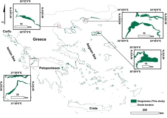
2.1. Study Site

The study area includes the Greek territorial waters—i.e., Ionian Sea and Greek part of the Aegean Sea—covering a total surface of 40,951 km² (Figure 1). We define this area on the basis of an edited 3-km buffer zone along the Greek coastline of approximately 18,000 km, following the results of [13] (see Section 2.3.2). The Aegean Sea features an intricate geomorphology that reflects past geologic history and recent geodynamic processes. Shallow shelves, deep basins, and troughs alternate throughout the buffer-defined area whose deepest point is ~2500 m (deepest area in the Aegean trench is ~ 5000 m). It has also a distinctive insular character with more than 1400 islands or islets, while its extensive coastline consists of several landforms, including sandy beaches, rocky shores, cliffs, coastal lagoons and deltaic systems, as well as a notable variety of coastal and marine habitat types. On the other hand, the Ionian Sea is considered an oligotrophic area, based both on low nutrient concentrations and primary production. Biological data reflect a very oligotrophic area, dominated by a microbial food web, where new production mostly derives from limited events in space and time, mainly driven by climatological factors generating mesoscale instabilities. In terms of biology, the Ionian Sea is influenced by the Adriatic water in the northern part of the subbasin, with higher phytoplankton biomass (particularly diatoms), while water of Atlantic origin makes up its southern part with the exception of the whole eastern side [19,20]. Seagrass meadows exist in protected bays and gulfs while their mean maximum depths of presence are between 25 and 35 m depending on the local conditions [21].

2.2. Satellite Data

We use Copernicus Sentinel-2 Level-1C (L1C) top of atmosphere (TOA) reflectance satellite data, the standard S2 archive in GEE. The available data extends from 23 June 2015 (date of launch of Sentinel-2A) to today with a 5-day temporal resolution (with the use of Sentinel-2B). For the present study, we choose a period between 1 September and 1 October 2017, which satisfies availability of both S2-A and S2-B imagery, and more importantly, a better-stratified water column in the study areas of Aegean and Ionian seas [18]. Our data input is the seven S2 bands: b1-coastal aerosol, b2—blue, b3—green, b4—red, b8—NIR, b11—SWIR1, and the QA60 band, the bitmask band which contains information on cloud mask. Bands b1 and QA60 are in 60-m spatial resolution, while b11 is in 20-m spatial resolution. GEE reprojects all to the 10-m native resolution of the b2, b3, b4, and b8. In total, 1045 S2 tiles—100 × 100 km² sub-images—compose our initial image dataset. All available datasets, from satellite images to field and auxiliary data are projected in the GCS WGS84 World Geodetic System.

2.3. Field Data

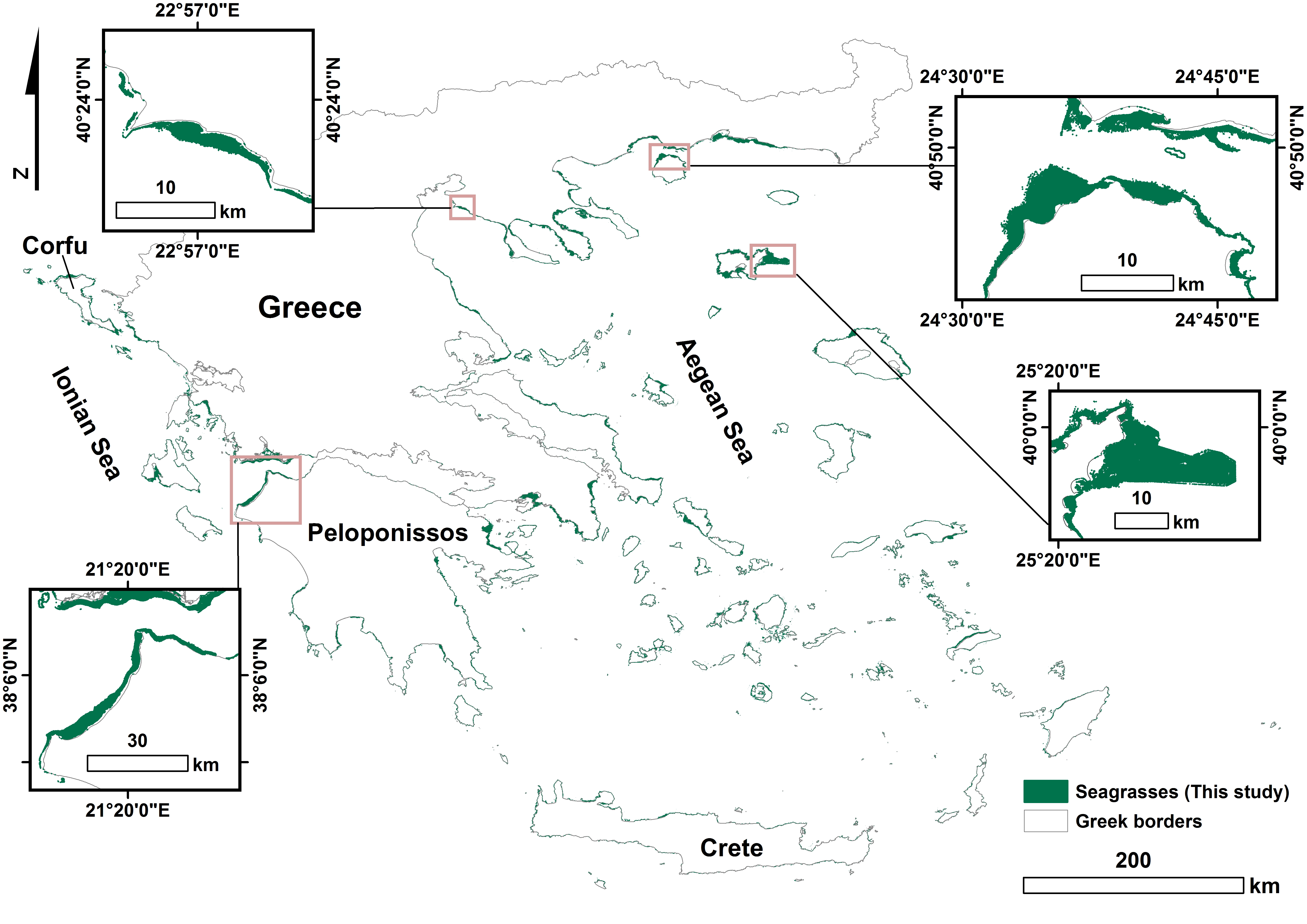
2.3.1. Training and Validation Data

We manually digitized all training data on very high spatial resolution images using the ArcGIS World Imagery base map (<60 cm pixel) (Figure 1). To ensure data quality, we selected areas in relative shallow waters where seagrass was easily interpreted. The digitization took place in areas where we have a high level of knowledge on the seabed cover and composition due to past and ongoing fieldwork activities. The nonseagrass class contained rocky, sandy, and deep-sea areas. To ensure consistency across all classes, we implement 4 × 4 homogeneous polygons (16 S2 pixels). In ArcGIS Desktop, the digitization tool allows to design polygon data with specific dimension and size. Thus, the size of each polygon is the same and the homogeneity is related to the seabed cover as this is identified by experienced image interpreters. In total, we used 1457 homogeneous polygons (23,312 pixels) for two classes (seagrass/nonseagrass) (Figure 2; Table 1). The homogeneity of all polygons is vital because their absence may cause misclassification. The validation data consists of 322 independent field data points based on unpublished data provided by terraSolutions m.e.r. (http://www.terrasolutions.eu/) to reduce bias.

2.3.2. Auxiliary Data

We utilize two additional auxiliary datasets to aid both the time (thus computing) efficiency of our processing chain and the distillation of its results. First, to mask out both land and deeper waters, we edit a shapefile of the Greek coastline at scale of 1:90,000 [22] by the Hellenic Navy Hydrographic Service (HNHS) in a two-step way; (a) we create a buffer of 3 km to encompass the whole optically shallow extent (where there is remote sensing signal from the seabed), (b) we manually edit the buffer of 3 km to include the deeper and/or larger meadows (according to the seagrass polygons of [13]) and to delete all the vertices over land. The resulted coastal area comprises our survey site of a total area of ~40,951 km². In addition, we use the bathymetry of the Aegean Sea for the post-classification stage (see Section 2.4.3). The Aegean Sea bathymetry depth zones (5-m intervals until 50-m depth) are fused products of HNHS, EMODnet (the European Marine Observation and Data Network), and in situ data collected during the ΜΑRItime Spatial planning for the protection and Conservation of the biodiversity in the Aegean sea (MARISCA) project [19].

2.4. Methodology

In addition to the easy and parallel access to the satellite image archives, GEE offers quick and adaptable computational tools for remotely sensed data processing and analysis. We exploit GEE tools to build our methodological chain, which is divided into three parts: (a) preclassification, (b) classification, (c) post-classification. Figure 3 displays this chain, while Figure 4 depicts its various successive stages.

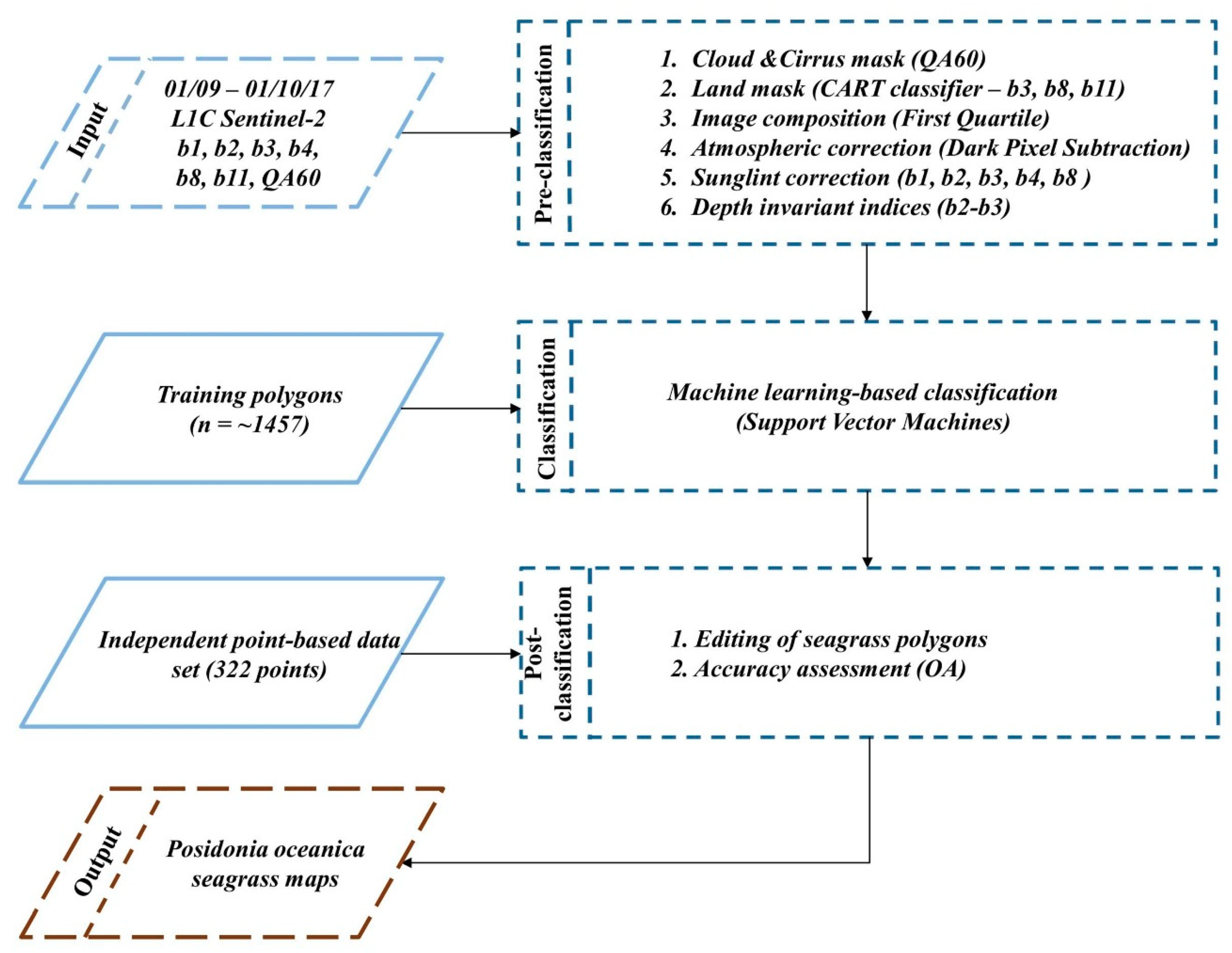
2.4.1. Preclassification

Our preclassification part consists of six steps:
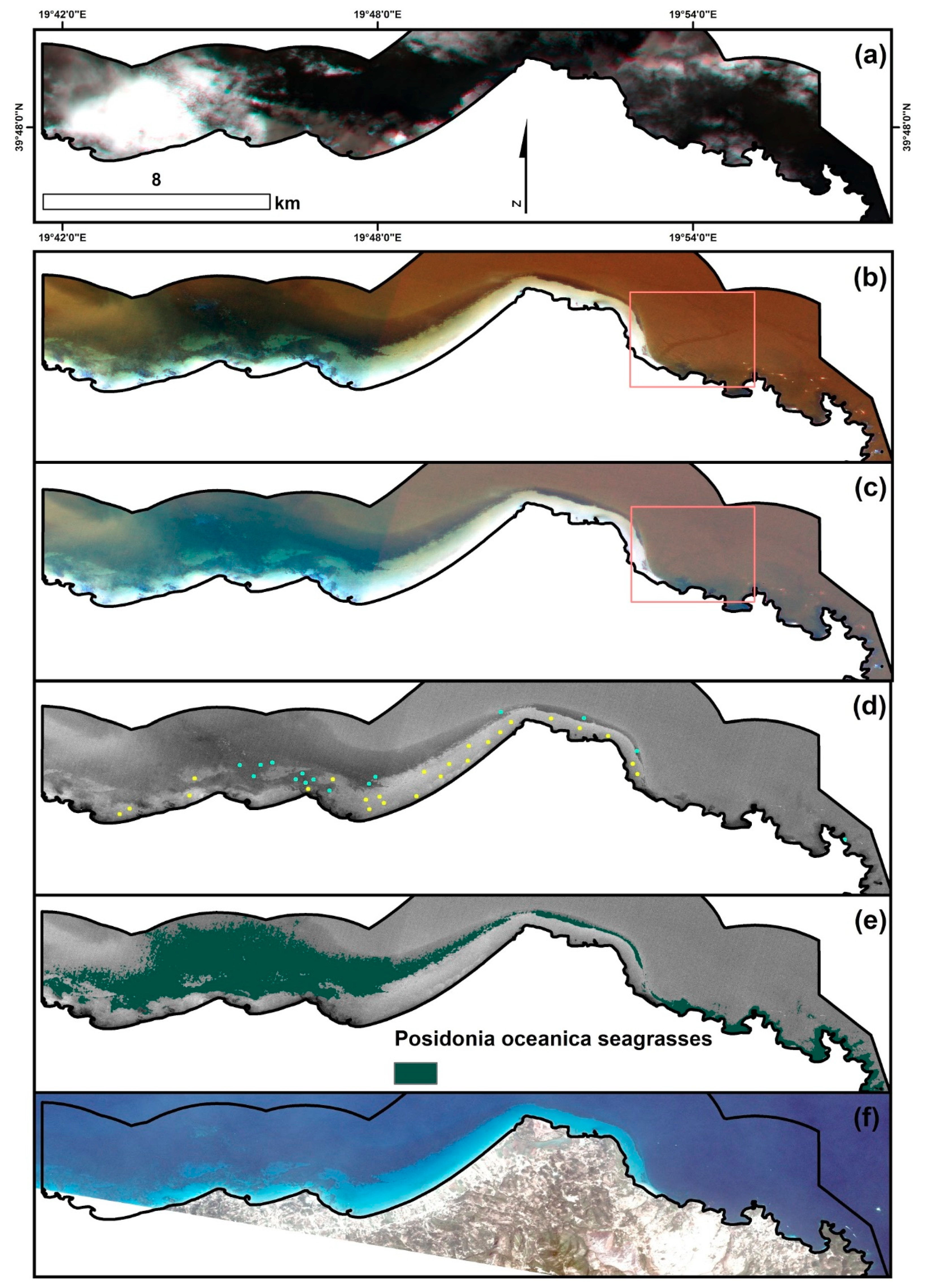
  • Cloud mask: We use the QA60 bitmask band to mask opaque and cirrus clouds and scale S2 L1C TOA images by 10,000 (Figure 4a,b).
  • Land mask: Although here we utilize the buffered coastline shapefile of Greek waters to mask out terrestrial Greece, we include a classification and regression tree (CART) classifier [23] in the GEE code that future users could employ to mask out their terrestrial part. The classifier is applied on a b3-b8-b11 composite and the user should train it with relevant pixels over land and water.
  • Image composition: We apply image composition which yields a new pseudo-image composite whose pixels are the first quartile (Q1) of the median values of the cloud corrected and masked for land images of step 2. The purpose of this approach is to decrease noncorrected image artefacts by the previous steps.
  • Atmospheric correction: We implement a modified dark pixel subtraction method following [24] to empirically address path radiance and noise in all sbands; this method subtracts the average reflectance and two standard deviations of optically deep water (>40 m) (Figure 4b).
  • Sunglint correction: We further correct the atmospherically corrected image composites with the sunglint correction algorithm of [25]. Following a user-defined set of pixels of variable sunglint intensity, the algorithms equals the corrected for sunglint composite to the initial first quartile composite minus the product of the regression slope of b8 against b1-b4 and the difference between b8 and its minimum value (Figure 4c).
  • Depth invariant indices calculation: To compensate the influence of variable depth on seabed habitats, we derive the depth invariant indices [26,27] for each pair of bands with reasonable water penetration (b1-b2, b2-b3, b1-b3) with the statistical analysis of [28]. Prior to the machine learning-based classification, we apply a 3 × 3 low pass filter in the depth invariant as well as the sunglint-corrected input to minimize remaining noise over the optically deep water extent which would have caused misclassified seagrass pixels otherwise (Figure 4d).

2.4.2. Classification

Although we experimented with three machine learning classifiers, support vector machines (SVM) [29], random forests (RF) [30], and CART [23], we end up using only SVM due to their better yielded classification output, both qualitatively and quantitatively (Figure 4e). Based on the statistical learning theory of [29], SVM solve linear and nonlinear classification problems by fitting a separating hyperplane to the training data of the studied classes; they take their name from the support vectors, namely the points closest to the hyperplane—the only ones that ultimately define it. A small number of studies have utilized SVM to map optically shallow habitats [31,32,33,34]. Here, we run SVM with a Gaussian radial basis function kernel (RBF), a parameter g, the width of the RBF, of 1000, and a regularization parameter, C, which governs the degree of acceptable misclassification, of 100. We empirically select the adequate pair values for g and C based on experiments that we run setting their range between a minimum of 0.01 and a maximum of 1000 using a multiplier of 10. Τhe input to the classifier is the sunglint-corrected S2 composite of b1, b2, b3, b4 and the depth invariant index b2-b3.

2.4.3. Post-Classification

The post-classification part consists of two components: the editing of seagrass polygons due to misclassified pixels as seagrass in deep water and the accuracy assessment of the these machine learning derived edited seagrass polygons. The accuracy assessment employs an independent validation data set (unpublished data from terraSolutions m.e.r.) consisting of 322 data points to reduce general bias. We report the overall accuracy of seagrass habitats in the extent of the Aegean and Ionian seas which is the ratio of the entire number of correctly classified pixels to the total number of validation pixels. The post-classification correction of seagrass pixels over deep water serves a better visualization of the classification output, but more significantly, it decreases the overprediction tendency of the classification results, namely seagrass area in the Aegean and Ionian seas; a single misclassified 10-m S2 pixel as P. oceanica seagrass would cause an overprediction of 100 m2.

3. Results

3.1. Preclassification

Regarding the preclassification steps, r2 of regression between sunglint-polluted b8 and b1-b4 composites are b1: 0.3, b2: 0.3, b3: 0.39, and b4: 0.39. As regards to the only herein employed depth invariant index of b2-b3 bands, the ratio of water attenuation coefficient is 0.57.

3.2. Classification

Our methodological workflow reveals that the seagrass area of the Greek Seas is 2510.1 km2; 1885 km2 in the Aegean Sea and 625 km2 in the Ionian Sea (Figure 5). As regards to individual geographical areas, the ones with the largest seagrass area (and maximum observed depth, where available, in parentheses) are Limnos (Figure 5d) with 254 km2 (40 m), NW Peloponissos (Figure 5c) with 99 km2, Corfu with 90 km2, Crete with 70 km2 (40 m), Thasos (Figure 5b) with 53 km2 (25 m), and the Thermaikos Gulf (Figure 5a) with 49 km2 (20 m). Across both seas, according to the employed auxiliary depth information, the depth of seagrass habitats is between 0 and 40 m.

3.3. Post-Classification

The observed overall accuracy of P. oceanica seagrass in both the Aegean and Ionian seas is 72% based on the independent field data set.

4. Discussion

4.1. On Global Mapping and Monitoring of Seagrasses, and the Results of the Present Case Study

The exponential increase in cloud-based computing power, machine learning algorithms, and freely available satellite image archives has rendered the vision of global-scale mapping and monitoring of seagrasses and their neighboring habitats more feasible than ever before. However, seagrass environments vary in regards to species composition and abundance, but also water clarity (secchi depth) which will influence the capability to apply approach globally. At present, while there are tangible efforts for the global monitoring of coral habitats [36], similar efforts focusing on seagrass ecosystems have been yet not envisioned.
Here, we have developed a methodological workflow within Google Earth Engine which employs a plethora of universally used algorithms in coastal aquatic habitat remote sensing along with image composition and machine learning that could potentially be applied to map and monitor seagrasses globally. We demonstrate its power along with its issues in the Greek Seas, namely the Aegean and Ionian Sea; in a total coastline extent of 40,951 km2, we map 2510.1 km2 of Greek seagrasses (Posidonia oceanica species) between 0 and 40 m of depth applying Support Vector Machines in a pixel-based fashion on 1045 Sentinel-2 tiles. In comparison to existing mapping efforts and known distribution of seagrasses in our study site, our area findings are ~4.2% less than the respective coverage estimations of [13] (2619.3 km2). This can be attributed to the different methods and data in use: pixel vs. object-based approach, different type of in situ data and difference in spatial resolution e.g., Sentinel-2 vs. Landsat-8 spatial resolution (10 vs. 30 m, respectively, resulting in a minimum mapping unit of 100 vs. 900 m2). A near-future regional comparison of pixel- to object-based approaches in the same context could shed further light upon the nature of their discrepancies—e.g., statistical vs. environmental. On the other hand, in comparison to the United Nations Environment Programme (UNEP) World Conservation Monitoring Centre (WCMC) Version 5 seagrass distribution, the herein seagrass area are nearly four times more (639.5 km2) [36].

4.2. The Good, the Bad, and the Best Practices of the Proposed Cloud-Based Workflow

The strength of our methodological chain lies mainly in the fact that it can be easily adjusted in space, time and data input. In comparison to the pre-processing chain of [18] and the therein use of the median value, we implement the first quartile here which yields less noisy image composites because it filters higher reflectances (=clouds and sunglint). The chain requires specific input to run:
(a)
Selection of a suitable time range; the suitability relates to possible available in situ data to run the machine learning classifiers, the atmospheric, water surface and column conditions of the study area, but also the season of maximum growth of the seagrass species of interest, especially for change detection studies. Here, we have chosen one month of Sentinel-2 imagery within the period of better water column stratification of the Greek Seas.
(b)
Selection of suitable points that will represent land and water for land masking (if needed), polygons over deep water (for atmospheric correction), variable sunglint intensity (for sunglint correction), and sandy seabed of variable depth (for the depth invariant index calculation).
(c)
Accurate in situ data that will cover all the existing habitats within the study extent for training of the machine learning classifications and validation with an ideally independent data set to reduce potential bias; here, we design remotely sensed, homogenous 4 × 4 (1600 m2) polygons for the training of the machine learning model and employ an independent point-based data set for the validation. We also decided to design deep-water polygons to minimize possible misclassifications with seagrasses.
In contrast, the weaknesses of the present workflow the following:
  • Method-wise, the herein image-based, empirical algorithms (e.g., dark pixel subtraction, sunglint correction, depth invariant indices) contain inherent assumptions in their nature and necessitate a sufficient selection of pixels to produce valuable results. Concerning the sunglint correction, specifically, an image composition spanning a large period of time can amplify the artificiality of the produced pseudo-composite, causing the sunglint correction algorithm to be unable to capture any existing interference by this phenomenon.
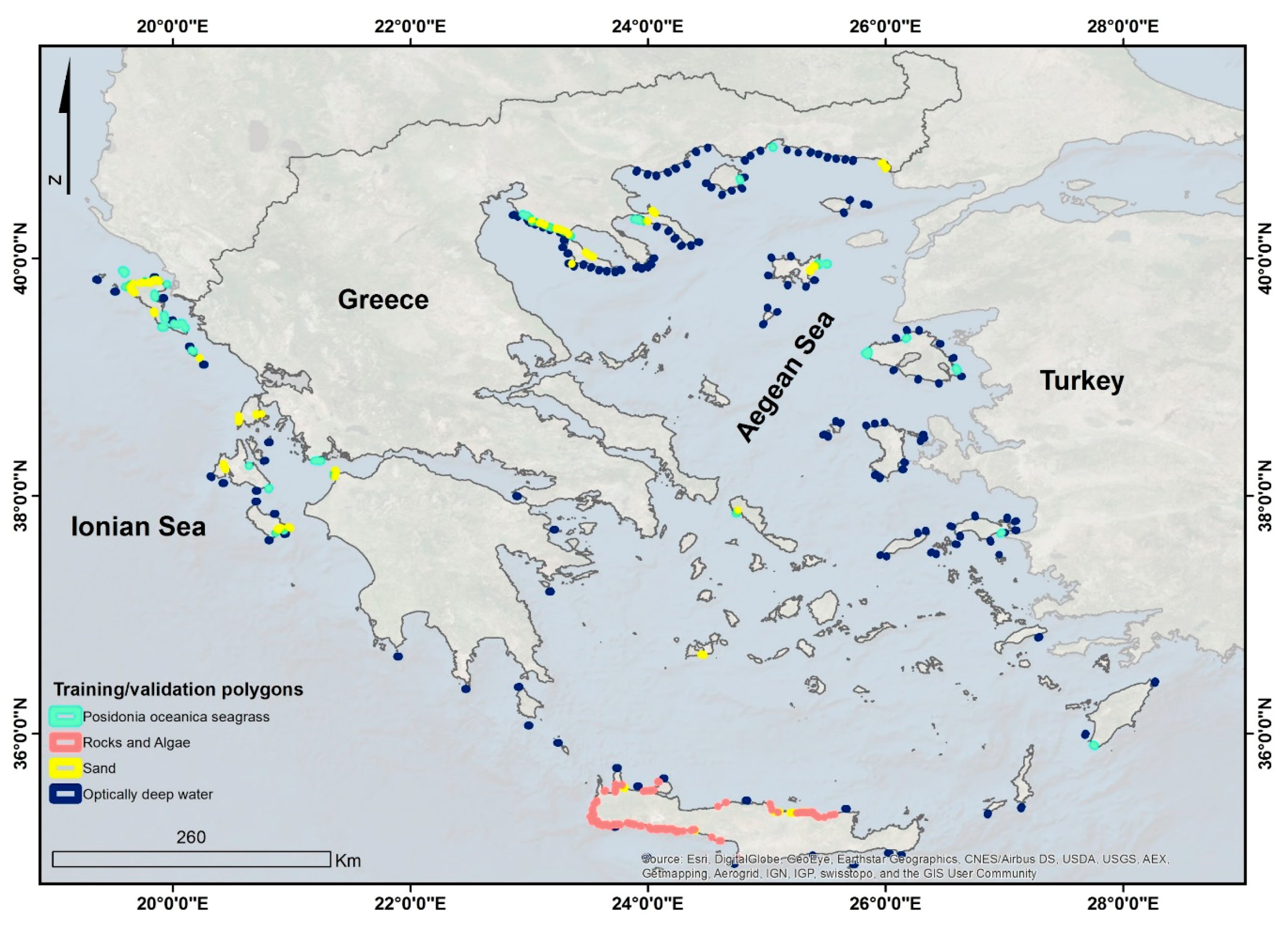
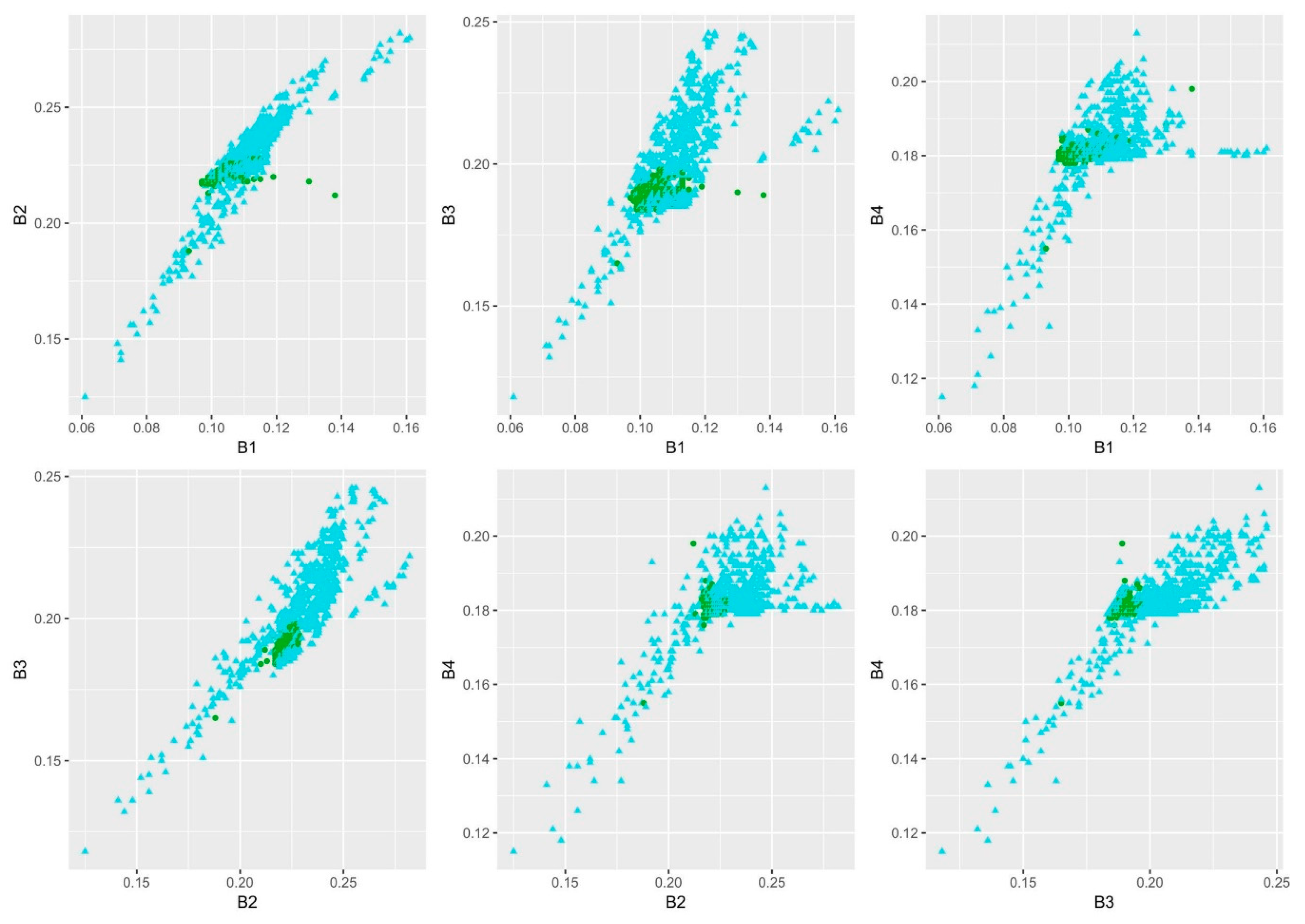
  • Data-wise, there is a threefold problem with Sentinel-2 applications in the remote sensing of optically shallow benthos and broadly aquatic extent. First, the tile limits of Sentinel-2 data are visible due to differences in viewing angles (odd and even detectors feature a different viewing angle) that produce striping. In turn, this artifact could severely impact classification output as it alters neighboring reflectances. A first possible solution for striping could be the application of pseudo-invariant feature normalization using a tile as a reference image and all the others as the slave ones—a theoretically, computationally expensive operation within GEE. A second solution is to split the initial study area into subareas—ultimately every tile within the visible stripes—where we could select polygons and run the classifier. The second data-related issue is the coastal aerosol band 1, which is originally in 60-m resolution in comparison to the 10-m resolution of all the other visible bands. Although on-the-fly reprojected to 10-m for visual purposes and integral towards coastal habitat mapping and SDB due to its great penetration, it causes artefacts upon application of the depth invariant indices of [26,27]. Therefore, we only utilise b2-b3 index during the classification step. This could be solved through the implementation of a downscaling approach of band 1 [37] into the existing workflow which is under exploration in terms of computation time efficiency. The third and last data-wise issue is the selection of training and validation data. We designed as homogeneous as possible polygons that represent seagrasses, sands, rocks, and deep water based on very high spatial resolution images; however, these will be as accurate as our experienced eye will dictate to us. Figure 2 shows that at all band-to-band scatterplots, the designed polygons of seagrass and non-seagrass beds are not well-differentiated and may have caused misclassifications. Generally, the collection of field data for the classification of remote sensing of aquatic habitats is expensive, time-consuming, and sparse today. More efforts should be driven towards allocating funding for accurate and high resolution in situ data and/or advocating the sharing of open datasets that would permit regional to global projects. The search for open access data on seagrass from relevant data repositories reveals a high number, however a fraction of these are potentially suitable for use in the remote sensing domain. Therefore, it is mandatory to urge a collaborative action between seagrass and remote sensing scientists, which will galvanize the development of a protocol that could be easily adapted in any seagrass bioregion for the designation of accurate and well documented with metadata, in situ data for seagrass mapping using the present workflow.

4.3. Future Endeavours

In addition to the much-needed availability of accurate in situ datasets suitable for image analysis of variable scales (from 50-cm to 30-m pixel size), we discuss three future endeavors following the use of the present cloud-based workflow:
  • Basin- (Mediterranean) to global-scale mapping and monitoring of seagrasses and related biophysical variables (specifically the climate change-related carbon sequestration): The expected lifespan of Sentinel-2 and its succeeding complementary twin mission (7.25 + 7.25 years) would unravel issues related to open and free, high spatial resolution data availability and allow intra-annual (seasonal) to interannual monitoring activities in the optically shallow grounds of seagrasses for 14.5 years by 2029, which marks the end of the announced UN decade of ocean science [38].
  • Improvement of certain stages of the present workflow: (a) Incorporation of a more sophisticated atmospheric correction algorithm like Py6S [39], (b) Implementation of optimization approaches for simultaneous derivation of benthic reflectance and bathymetry based on the semianalytical inversion model of [40,41], (c) Inclusion of best available pixel (BAP) approach within span of well-stratified column period which use pixel-based scores, according to both atmospheric-, season- and sensor-related issues, to produce a composite with the best available pixel [42], (d) Incorporation of object-based segmentation and classification methods to improve classified outputs. The main drawback of the first three improvements is they would possibly lower the time efficiency of the present version of the chain due to the higher demand in computational power based on the need to implement look up tables and/or run radiative transfer codes.
  • Integration of seagrasses and other coastal habitats to the analysis ready data (ARD) era: Recent advances in optical multispectral remote sensing (e.g., Sentinel-2, Landsat 8, Planet’s Doves), cloud computing and machine learning classifiers can enable multiscale, multitemporal and sensor-agnostic approaches where all the aforementioned data will be preprocessed to a high scientific standard (Cloud Optimized GeoTIFF; [43]), further harnessing past, present and future remotely sensed big data and facilitating the near real-time measurements of physical changes of these immensely valuable habitats for Earth.

5. Conclusions

The present study introduces a complete methodological workflow for large-scale, high spatial and temporal mapping and monitoring of seagrasses and other optically shallow habitats. The workflow can be easily tuned to spatial, timely and data input; here, we showcase its large spatiotemporal and time efficiency, mapping 2510.1 km2 of P. oceanica seagrasses in 40,951 km2 of the Greek Seas utilizing a 10-m Sentinel-2 based composite of 1045 tiles in seconds. The workflow could also ingest the freely available image archive of Landsat-8 surface reflectance as input. We envisage that the herein adaptable, accurate, and time- and cost efficient cloud-based workflow will provide the vital seasonal to interannual baseline mapping and the monitoring of seagrass ecosystems on a global scale, identifying problematic areas, resolving current trends, and assisting coastal conservation, management planning, and ultimately climate change mitigation.

Author Contributions

D.T. conceived the idea; D.T., D.P. and B.A. designed the remotely sensed in situ data; D.T., D.P., and K.T. wrote the paper; B.A. wrote the code in Google Earth Engine; K.T., N.C. and P.R supervised the development of the present workflow and paper, from start to finish.

Funding

D.P. and N.C. are supported by the European H2020 Project 641762 ECOPOTENTIAL: Improving future ecosystem benefits through Earth Observations. D.T. is supported by a DLR-DAAD Research Fellowship (No. 57186656). B.A. is supported by GF-KTR 2472040.

Acknowledgments

This work contributed to and was partially supported by the European H2020 Project 641762 ECOPOTENTIAL: Improving future ecosystem benefits through Earth Observations. Dimosthenis Traganos is supported by a DLR-DAAD Research Fellowship (No. 57186656).

Conflicts of Interest

The authors declare no conflicts of interest.

References

  1. Short, F.T.; Dennison, W.C.; Carruthers, T.J.B.; Waycott, M. Global seagrass distribution and diversity: A bioregional model. J. Exp. Mar. Biol. Ecol. 2007, 350, 3–20. [Google Scholar] [CrossRef]
  2. Green, E.P.; Short, F.T. World Atlas of Seagrasses; University of California Press: Berkeley, CA, USA, 2003. [Google Scholar]
  3. Duarte, C.M.; Borum, J.; Short, F.T.; Walker, D.I. Seagrass Ecosystems: Their Global Status and Prospects. In Aquatic Ecosystems: Trends and Global Prospects; Polunin, N., Ed.; Cambridge University Press: Cambridge, UK, 2008. [Google Scholar] [CrossRef]
  4. Nordlund, M.L.; Koch, E.W.; Barbier, E.B.; Creed, J.C. Seagrass Ecosystem Services and Their Variability across Genera and Geographical Regions. PLoS ONE 2016, 11, e0163091. [Google Scholar] [CrossRef] [PubMed]
  5. Githaiga, M.N.; Kairo, J.G.; Gilpin, L.; Huxham, M. Carbon storage in the seagrass meadows of Gazi Bay, Kenya. PLoS ONE 2017, 12, e0177001. [Google Scholar] [CrossRef] [PubMed]
  6. Fourqurean, J.W.; Duarte, C.M.; Kennedy, H.; Marbà, N.; Holmer, M.; Mateo, M.A.; Apostolaki, E.T.; Kendrick, G.A.; Krause-Jensen, D.; McGlathery, K.J.; et al. Seagrass ecosystems as a globally significant carbon stock. Nat. Geosci. 2012, 5, 505–509. [Google Scholar] [CrossRef]
  7. UN General Assembly, Transforming Our World: The 2030 Agenda for Sustainable Development. 21 October 2015. Available online: http://www.refworld.org/docid/57b6e3e44.html (accessed on 3 August 2018).
  8. Waycott, M.; Carlos, M.D.; Carruthers, T.J.B.; Orth, R.J.; Dennison, W.C.; Olyarnik, S.; Calladine, A.; Fourqurean, J.W.; Heck, K.L.J.; Hughes, A.R.; et al. Accelerating loss of seagrasses across the globe threatens coastal ecosystems. Proc. Natl. Acad. Sci. USA 2009, 106, 12377–12381. [Google Scholar] [CrossRef] [PubMed] [Green Version]
  9. Orth, R.J.; Carruthers, T.J.; Dennison, W.C.; Duarte, C.M.; Fourqurean, J.W.; Heck, K.L.; Hughes, A.R.; Kendrick, G.A.; Kenworthy, W.J.; Olyarnik, S.; et al. A global crisis for seagrass ecosystems. Bioscience 2006, 56, 987–996. [Google Scholar] [CrossRef]
  10. Hossain, M.S.; Bujang, J.S.; Zakaria, M.H.; Hashim, M. The application of remote sensing to seagrass ecosystems: An overview and future research prospects. Int. J. Remote Sens. 2015, 36, 61–114. [Google Scholar] [CrossRef]
  11. Hedley, J.D.; Roelfsema, C.M.; Chollett, I.; Harborne, A.R.; Heron, S.F.; Weeks, S.; Skirving, W.J.; Strong, A.E.; Eakin, C.M.; Christensen, T.R.L.; et al. Remote Sensing of Coral Reefs for Monitoring and Management: A Review. Remote Sens. 2016, 8, 118. [Google Scholar] [CrossRef]
  12. Wabnitz, C.; Andréfouët, S.; Torres-Pulliza, D.; Müller-Karger, F.; Kramer, P. Regional-scale seagrass habitat mapping in the wider Caribbean region using Landsat sensors: Applications to conservation and ecology. Remote Sens. Environ. 2008, 112, 3455–3467. [Google Scholar] [CrossRef]
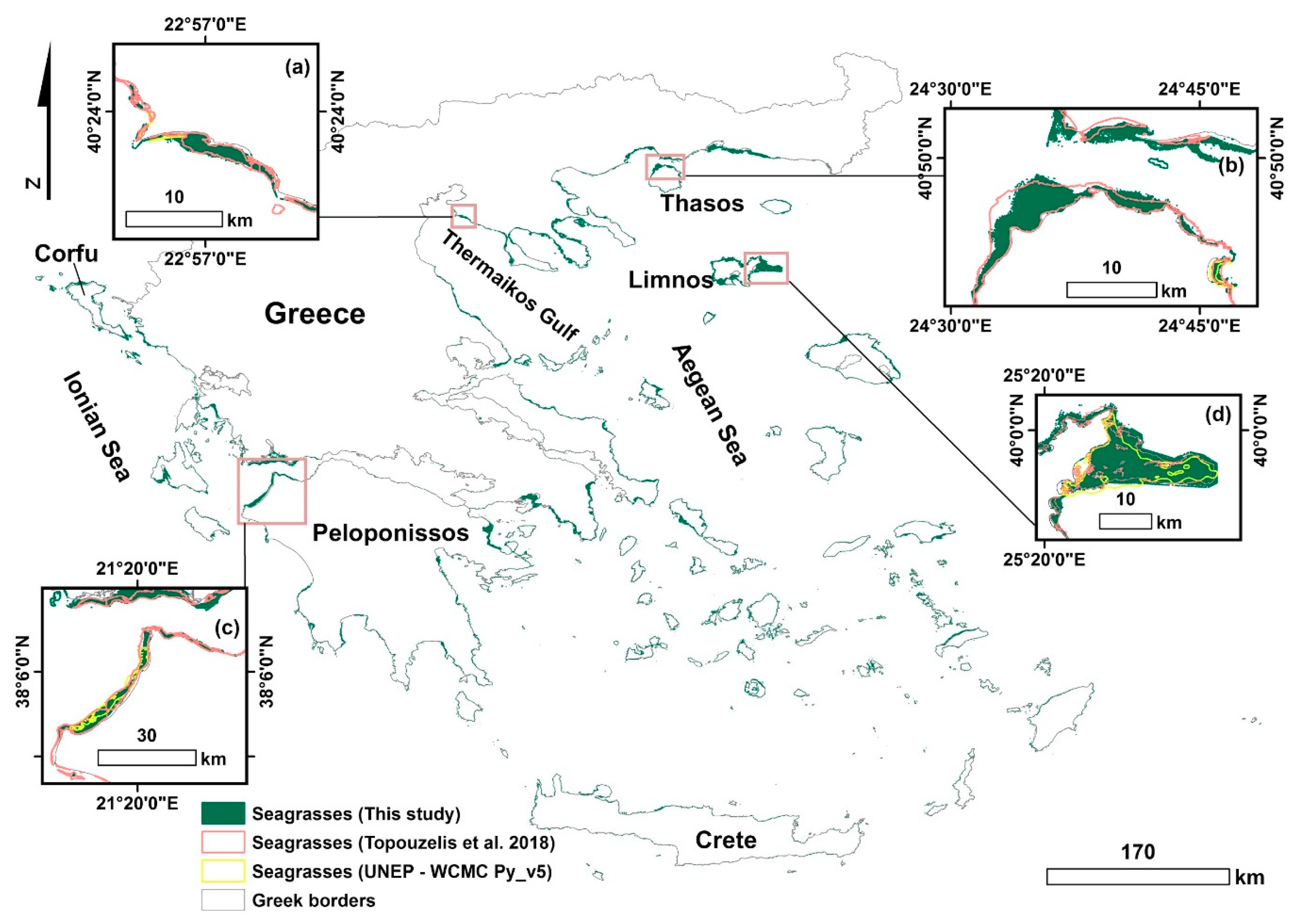
  13. Topouzelis, K.; Makri, D.; Stoupas, N.; Papakonstantinou, A.; Katsanevakis, S. Seagrass mapping in Greek territorial waters using Landsat-8 satellite images. Int. J. Appl. Earth Obs. Geoinform. 2018, 67, 98–113. [Google Scholar] [CrossRef]
  14. Roelfsema, C.M.; Kovacs, E.; Phinn, S.R.; Lyons, M.; Saunders, M.; Maxwell, P. Challenges of Remote Sensing for Quantifying Changes in Large Complex Seagrass Environments. Estuar. Coast. Shelf Sci. 2013, 133, 161–171. [Google Scholar] [CrossRef]
  15. Hansen, M.C.; Potapov, P.V.; Moore, R.; Hancher, M.; Turubanova, S.A.A.; Tyukavina, A.; Thau, D.; Stehman, S.V.; Goetz, S.J.; Loveland, T.R.; et al. High-Resolution Global Maps of 21st-Century Forest Cover Change. Science 2013, 342, 850–853. [Google Scholar] [CrossRef] [PubMed]
  16. Xiong, J.; Thenkabail, P.S.; Gumma, M.K.; Teluguntla, P.; Poehnelt, J.; Congalton, R.G.; Yadav, K.; Thau, D. Automated cropland mapping of continental Africa using Google earth engine cloud computing. ISPRS J. Photogramm. Remote Sens. 2017, 126, 225–244. [Google Scholar] [CrossRef]
  17. Pekel, J.F.; Cottam, A.; Gorelick, N.; Belward, A.S. High-resolution mapping of global surface water and its long-term changes. Nature 2016, 540, 418–422. [Google Scholar] [CrossRef] [PubMed]
  18. Traganos, D.; Poursanidis, D.; Aggarwal, B.; Chrysoulakis, N.; Reinartz, P. Estimating Satellite-Derived Bathymetry (SDB) with the Google Earth Engine and Sentinel-2. Remote Sens. 2018, 10, 859. [Google Scholar] [CrossRef]
  19. Sini, M.; Katsanevakis, S.; Koukourouvli, N.; Gerovasileiou, V.; Dailianis, T.; Buhl-Mortensen, L.; Damalas, D.; Dendrinos, P.; Dimas, X.; Frantzis, A.; et al. Assembling Ecological Pieces to Reconstruct the Conservation Puzzle of the Aegean Sea. Front. Mar. Sci. 2017, 4. [Google Scholar] [CrossRef] [Green Version]
  20. Casotti, R.; Landolfi, A.; Brunet, C.; Ortenzio, F.D.; Mangoni, O.; Ribera d’Alcala, M. Composition and dynamics of the phytoplankton of the Ionian Sea (eastern Mediterranean). J. Geophys. Res. 2003, 108. [Google Scholar] [CrossRef] [Green Version]
  21. Gerakaris, V.; Panayotidis, P.; Tsiamis, K.; Nikolaidou, A.; Economou-Amili, A. Posidonia oceanica meadows in Greek seas: Lower depth limits and meadow densities. In Proceedings of the 5th Mediterranean Symposium on Marine Vegetation, Portorož, Slovenia, 27–28 October 2014. [Google Scholar]
  22. HNHS. Greek Coastline at Scale 1:90,000. 2018. Available online: https://www.hnhs.gr/en/?option=com_opencart&Itemid=268&route=product/product&path=86&producp_id=271 (accessed on 3 August 2018).
  23. Breiman, L.; Friedman, J.H.; Olshen, R.A.; Stone, C.J. Classification and Regression Trees. In Chapman and Hall/CRC; CRC Press: Boca Raton, FL, USA, 1984. [Google Scholar]
  24. Armstrong, R.A. Remote sensing of submerged vegetation canopies for biomass estimation. Int. J. Remote Sens. 1993, 14, 621–627. [Google Scholar] [CrossRef]
  25. Hedley, J.D.; Harborne, A.R.; Mumby, P.J. Technical note: Simple and robust removal of sun glint for mapping shallow-water benthos. Int. J. Remote Sens. 2005, 26, 2107–2112. [Google Scholar] [CrossRef]
  26. Lyzenga, D.R. Passive remote sensing techniques for mapping water depth and bottom features. Appl. Opt. 1978, 17, 379–383. [Google Scholar] [CrossRef] [PubMed]
  27. Lyzenga, D.R. Remote sensing of bottom reflectance and water attenuation parameters in shallow water using aircraft and Landsat data. Int. J. Remote Sens. 1981, 2, 71–82. [Google Scholar] [CrossRef]
  28. Green, E.P.; Mumby, P.J.; Edwards, A.J.; Clark, C.D. Remote Sensing Handbook for Tropical Coastal Management; UNESCO Press: Paris, France, 2000; pp. 1–316. [Google Scholar]
  29. Vapnik, V. The Nature of Statistical Learning Theory; Springer Press: New York, NY, USA, 1995. [Google Scholar]
  30. Breiman, L. Random forests. Mach. Learn. 2001, 45, 5–32. [Google Scholar] [CrossRef]
  31. Zhang, C. Applying data fusion techniques for benthic habitat mapping and monitoring a coral reef ecosystem. ISPRS J. Photogramm. Remote Sens. 2015, 104, 213–223. [Google Scholar] [CrossRef]
  32. Traganos, D.; Reinartz, P. Mapping Mediterranean Seagrasses with Sentinel-2 Imagery. Available online: https://www.sciencedirect.com/science/article/pii/S0025326X17305726 (accessed on 3 August 2018).
  33. Traganos, D.; Cerra, D.; Reinartz, P. CubeSat-Derived Detection of Seagrasses Using Planet Imagery Following Unmixing-Based Denoising: Is Small the Next Big? Available online: https://www.int-arch-photogramm-remote-sens-spatial-inf-sci.net/XLII-1-W1/283/2017/isprs-archives-XLII-1-W1-283-2017.pdf (accessed on 3 August 2018).
  34. Poursanidis, D.; Topouzelis, K.; Chrysoulakis, N. Mapping coastal marine habitats and delineating the deep limits of the Neptune’s seagrass meadows using VHR earth observation data. Int. J. Remote Sens. 2018. [Google Scholar] [CrossRef]
  35. The UN Environment World Conservation Monitoring Centre (UNEP-WCMC). Global Distribution of Seagrasses (Version 5.0). Fourth Update to the Data Layer Used in Green and Short (2003). 2017. Available online: http://data.unep-wcmc.org/datasets/7 (accessed on 3 August 2018).
  36. Partnership to Develop First-Ever Global Map and Dynamic Map of Coral Reefs. 2018. Available online: https://carnegiescience.edu/node/2354 (accessed on 3 August 2018).
  37. Brodu, N. Super-Resolving Multiresolution Images with Band-Independent Geometry of Multispectral Pixels. IEEE Trans. Geosci. Remote Sens. 2017, 55, 4610–4617. [Google Scholar] [CrossRef]
  38. UNESCO. United Nations Decade of Ocean Science for Sustainable Development (2021–2030). 2018. Available online: https://en.unesco.org/ocean-decade (accessed on 3 August 2018).
  39. Wilson, R. Py6S—A Python Interface to 6S. 2012. Available online: https://py6s.readthedocs.io/en/latest/ (accessed on 3 August 2018).
  40. Lee, Z.; Carder, K.L.; Mobley, C.D.; Steward, R.G.; Patch, J.S. Hyperspectral remote sensing for shallow waters: 1. A semianalytical model. Appl. Opt. 1998, 37, 6329–6338. [Google Scholar] [CrossRef] [PubMed]
  41. Lee, Z.; Carder, K.L.; Mobley, C.D.; Steward, R.G.; Patch, J.S. Hyperspectral remote sensing for shallow waters: 2. Deriving bottom depths and water properties by optimization. Appl. Opt. 1999, 38, 3831–3843. [Google Scholar] [CrossRef] [PubMed]
  42. White, J.C.; Wulder, M.A.; Hobart, G.W.; Luther, J.E.; Hermosilla, T.; Griffiths, P.; Coops, N.C.; Hall, R.J.; Hostert, P.; Dyk, A.; et al. Pixel-based image compositing for large-area dense time series applications and science. Can. J. Remote Sens. 2014, 40, 192–212. [Google Scholar] [CrossRef]
  43. Cloud Optimized GeoTIFF. An Imagery Format for Cloud-Native Geospatial Processing. 2018. Available online: http://www.cogeo.org/ (accessed on 3 August 2018).
Figure 1. Geographical location of survey site and training polygons of the herein considered classes. All polygons are in Geographic Coordinate System (CGS) World Geodetic System (WGS) 84 World Geodetic System.
Remotesensing 10 01227 g001
Figure 2. Scatter plots of the first four, sunglint-corrected Sentinel-2 bands depicting waveband reflectivity of the herein 1457 polygons for the whole extent of the study area. Seagrasses are in green circles and nonseagrasses are in light blue triangles.
Remotesensing 10 01227 g002
Figure 3. Methodological workflow of the present study within Google Earth Engine. OA denotes overall accuracy. In the present study we did not implement step 2 (due to the use of a coastline buffer), however, we include it as it is an important component of the methodological chain.
Remotesensing 10 01227 g003
Figure 4. Successive stages of the developed workflow through the resulting false-color (b1-b2-b3) Sentinel-2 composites. (a) Initial S2, (b) cloud- and atmospherically-corrected, (c) sunglint-corrected, (d) depth invariant index b2-b3, (e) support vector machines-based classified product draped over the b2-b3 depth invariant index layer, (f) PlanetScope surface reflectance product (as imaged by Planet’s Doves) in natural color for high resolution reference (3 m) (ID: 20170828_084352_100e/20170828_084352_100e_3B_AnalyticMS_SR). The pink squares indicate sunglint presence in (b) and its correction in (c). Τhe green and yellow polygons show employed seagrass and sand pixels in the machine learning classification. All panels are in GCS WGS84 World Geodetic System.
Remotesensing 10 01227 g004
Figure 5. Distribution of seagrasses in the Greek Seas. (a) Thermaikos Gulf, (b) Thasos Island, (c) NE Peloponissos, (d) Limnos Island. Inset maps contain results from [13,35] for reference and further validation of our results. All panels are in GCS WGS84 World Geodetic System.
Remotesensing 10 01227 g005
Table 1. Number of implemented polygons and pixels per class for our ~40,951 km² survey site.
ClassPolygonsPixels%
Seagrass329526422.6
Nonseagrass112818,04877.4
Sum145723,312100

