Leveraging the Google Earth Engine for Drought Assessment Using Global Soil Moisture Data

1
Hydrological Sciences Branch, NASA Goddard Space Flight Center, Greenbelt, MD 20706, USA
2
Science Application International Corporation (SAIC), Lanham, MD 20706, USA
3
Earth System Science Interdisciplinary Center, University of Maryland, College Park, MD 20742, USA
*
Author to whom correspondence should be addressed.
Remote Sens. 2018, 10(8), 1265; https://doi.org/10.3390/rs10081265
Submission received: 29 June 2018
/
Revised: 27 July 2018
/
Accepted: 8 August 2018
/
Published: 11 August 2018
(This article belongs to the Collection Google Earth Engine Applications)
Abstract
:Soil moisture is considered to be a key variable to assess crop and drought conditions. However, readily available soil moisture datasets developed for monitoring agricultural drought conditions are uncommon. The aim of this work is to examine two global soil moisture datasets and a set of soil moisture web-based processing tools developed to demonstrate the value of the soil moisture data for drought monitoring and crop forecasting using the Google Earth Engine (GEE). The two global soil moisture datasets discussed in the paper are generated by integrating the Soil Moisture Ocean Salinity (SMOS) and Soil Moisture Active Passive (SMAP) missions’ satellite-derived observations into a modified two-layer Palmer model using a one-dimensional (1D) ensemble Kalman filter (EnKF) data assimilation approach. The web-based tools are designed to explore soil moisture variability as a function of land cover change and to easily estimate drought characteristics such as drought duration and intensity using soil moisture anomalies and to intercompare them against alternative drought indicators. To demonstrate the utility of these tools for agricultural drought monitoring, the soil moisture products and vegetation- and precipitation-based products were assessed over drought-prone regions in South Africa and Ethiopia. Overall, the 3-month scale Standardized Precipitation Index (SPI) and Normalized Difference Vegetation Index (NDVI) showed higher agreement with the root zone soil moisture anomalies. Soil moisture anomalies exhibited lower drought duration, but higher intensity compared with SPIs. Inclusion of the global soil moisture data into the GEE data catalog and the development of the web-based tools described in the paper enable a vast diversity of users to quickly and easily assess the impact of drought and improve planning related to drought risk assessment and early warning. The GEE also improves the accessibility and usability of the earth observation data and related tools by making them available to a wide range of researchers and the public. In particular, the cloud-based nature of the GEE is useful for providing access to the soil moisture data and scripts to users in developing countries that lack adequate observational soil moisture data or the necessary computational resources required to develop them.
1. Introduction
The remote sensing advances made over the past three decades have radically improved our ability to obtain routine, global information about the amount of water present in the soil [1,2,3]. Several well-evaluated soil moisture (SM) datasets have proven useful for a wide range of applications, including weather and climate forecasting, monitoring of drought and wildfires, tracking floods and landslides, and enhanced agricultural productivity [4,5,6,7]. Despite all the advantages satellite-based soil moisture monitoring offers, such as global coverage, high accuracy, and high temporal frequency essential for operational applications, the shallow penetration depth of the microwave frequencies used for soil moisture monitoring remains a limiting factor [3]. In fact, many hydrological processes and forecasting and decision-making activities linked to soil moisture require knowledge of the root zone soil moisture (RZSM) information. The latter is typically estimated using hydrologic land surface models, which are traditionally driven by some weather-related observations such as precipitation, temperature, and so forth. The credibility of the modeled RZSM estimates is strongly dependent on the quality of the forcing data [8,9].
Hydrologic data assimilation (DA) offers a way to reduce the impact of precipitation-related errors and enhance the quality of the modeled RZSM data by integrating satellite-based observations into the model. It is essentially an optimal merging technique that results in an enhanced analysis product with improved accuracy over either of the parent products alone (i.e., the model data and the satellite observations). This paper focuses on the value of a combined model-satellite soil moisture dataset for near-real time drought and crop condition monitoring, developed in an effort to improve the RZSM information used by the United States Department of Agriculture-Foreign Agricultural Services (USDA-FAS).
One of the operational objectives of the USDA-FAS is the development of global crop yield forecasts, which heavily employ modeled soil moisture to force crop yield models. These forecasts are generated utilizing information from the Crop Condition Data Retrieval and Evaluation database management system, where soil moisture is an essential indicator used to assess crop health and monitor drought conditions and evaluate their impact on expected end of season yields. The baseline USDA-FAS RZSM information is generated using the modified Palmer model (PM), which is a relatively simple two-layer water balance model driven by daily estimates of precipitation and temperature [10,11]. The PM is highly susceptible to the quality of the precipitation forcing data, which are more error-prone over poorly instrumented areas [8]. Over a decade of research conducted in collaboration with USDA-FAS demonstrated that the agency’s model-based RZSM estimates produced by the PM can be improved by assimilating satellite-derived observations [11,12]. Here, we focus on the operational implementation of the DA-enhanced PM using soil moisture retrievals from two passive microwave missions, the European Space Agency (ESA)’s Soil Moisture and Ocean Salinity (SMOS) [13] mission and the National Aeronautics Space Agency (NASA)’s Soil Moisture Active Passive (SMAP) mission [14] which launched in 2009 and 2015 respectively, specifically designed to monitor near-surface soil moisture at a global scale using L-band frequency.
The goal of this paper is to announce the availability of these global soil moisture datasets and to demonstrate their value for drought monitoring using the Google Earth Engine (GEE). The GEE is a web-based service that stores a petabyte archive of Earth observations and related data and provides an efficient processing software, which enables users to develop complex geospatial analyses and visualizations utilizing high-performance computing resources. The GEE capabilities have been utilized for a range of applications, including soil mapping, malaria risk assessment, and automated cropland mapping [15,16,17,18]. In this study, we demonstrate the value of the SMOS- and SMAP-datasets and the web-based tools utilizing the global soil moisture dataset generated using the satellite-enhanced PM available in the GEE data catalog. The GEE and the available tools enable users to acquire, process, analyze, and visualize Earth observing data rapidly for any user-specified region across the globe without downloading and processing a large volume of data on the user’s desktop. The web-based drought assessment tools alleviate the need for users to install and work with desktop data managing and processing software, which are often labor intensive, time consuming, and difficult to reproduce, thereby overcoming compatibility limitations and enhancing usability and reproducibility of the analyses and results.
The paper is organized as follows: Section 2 provides a detailed description of the soil moisture data, modeling approach, and preparation steps for integrating the data into the GEE platform; Section 3 focuses on the functionality of the GEE tools developed for drought assessment using the satellite-enhanced PM global soil moisture data; Section 4 describes the application of the GEE tools over South Africa and Ethiopia; and Section 5 and Section 6 provide some discussion of the results and conclusions, respectively.
2. Data Processing for the Google Earth Engine Platform
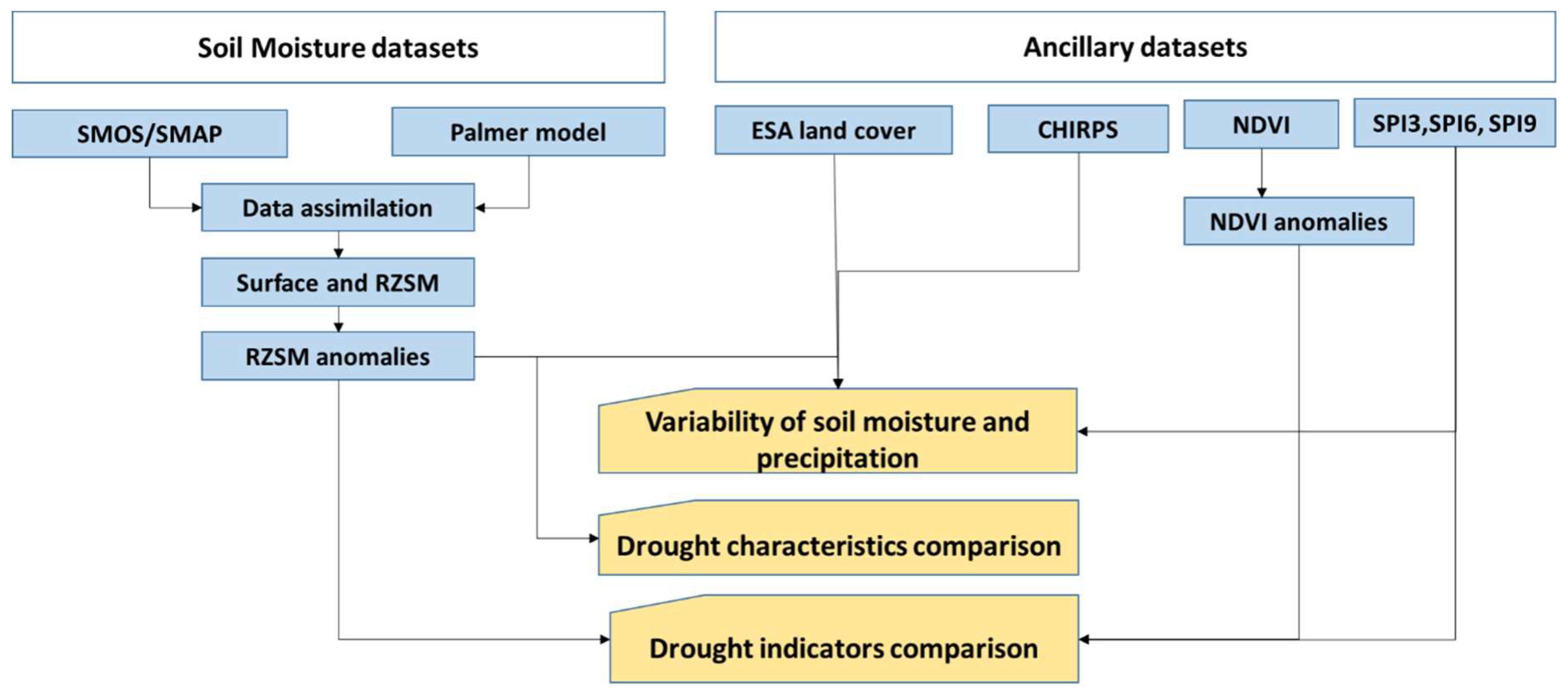
An overview of the major methodological steps applied in this study is provided in Figure 1. First, we processed satellite-based soil moisture datasets to estimate surface and RZSM and their anomalies. Then, we used RZSM and precipitation data to explore their spatial and temporal variability with different land cover types. Next, we estimated drought characteristics from RZSM anomalies and compare against other alternative drought indices. Details about these datasets are provided in Table 1. One of the primary goals of this study is to introduce global soil moisture data sets in the GEE; hence we provide detailed descriptions of the soil moisture datasets in the following sub-section.
2.1. Soil Moisture Data Set
The USDA-FAS Soil Moisture System: Palmer Model, Data Assimilation, and Satellite Observations
- a. Theoretical Basis
The two-layer Palmer Model used by the USDA-FAS is a bookkeeping water balance model that accounts for the water gained by precipitation and lost by evapotranspiration [10]. The top layer is assumed to have 2.54 cm available water-holding capacity at saturation, while the holding capacity of the lower layer varies depending on the depth of the bedrock. The model is driven by daily precipitation data and daily minimum and maximum temperature observations provided by the United States (U.S.) Air Force 557th Weather Wing (formerly known as the U.S. Air Force Weather Agency, AFWA). The AFWA dataset is derived using multiple sources, inducting remotely sensed observations and gauge data acquired from the World Meteorological Organization (WMO). The model is enhanced by adding a data assimilation unit, which allows the routine integration of satellite-based observations into the model using a one-dimensional (1D) ensemble Kalman filter approach (EnKF) [11,12]. The purpose of this modification is to improve the PM RZSM information by integrating the added values of the surface soil moisture retrievals to the model and examining their potential to correct for meteorological forcing uncertainty. A detailed description of Bayesian theory-based filtering, including the EnKF is beyond the scope of this paper; however, the methods are well established and documented [25,26,27,28,29].
The Kalman filter is a sequential Monte Carlo assimilation technique, where the model forecasts are optimally updated in response to the satellite observations via the Kalman gain (K). The operational implementation of EnKF requires some knowledge of the model uncertainty (Q) and the error of the satellite observations (R). Here, both of these parameters have been parameterized using some a priori knowledge. Given the above-discussed and well-established dependence of the model accuracy on the uncertainty of the rainfall data and the fact that the AFWA rainfall dataset is rain-gauge corrected, R has been modeled as a function of proximity to the WMO gauge station. Q, on the other hand, has been parameterized as a land cover type using published accuracy assessment analysis [30,31,32,33,34,35,36]. We discuss the implementation of the satellite-enhanced PM using remotely sensed observations acquired from two L-band missions, SMOS and SMAP. Full technical descriptions of these missions can be found in [13], respectively.
The corresponding SMOS and SMAP soil moisture estimates assimilated into the PM are derived using slightly different retrieval approaches; however, both systems and soil moisture products show similar performance and overall accuracy [37,38]. The global SMOS soil moisture data are operationally acquired from the National Oceanic and Atmospheric Administration (NOAA) Soil Moisture Operational Products System (SMOPS), which are distributed at 0.25° grid spacing (https://data.nodc.noaa.gov/cgi-bin/iso?id=gov.noaa.ncdc:C00994; last accessed on May 2018). SMAP offers a variety of soil moisture products (https://smap.jpl.nasa.gov/data/; last accessed on May 2018). This study applies the L3 passive-only SMAP soil moisture product. The data are routinely downloaded from the National Snow and Ice Data Center (https://nsidc.org/data/SPL3SMP/versions/4; last accessed on May 2018). SMAP is distributed in Equal-Area Scalable Earth (EASE)-grid 2 projection at 36-km grid spacing; therefore, the data have been pre-processed to match the model grid of 0.25°.
- b. Operational Implementation
The satellite enhanced Palmer Model is set to run operationally on NASA’s Global Inventory Modeling and Mapping Studies (GIMMS) Global Agricultural Monitoring (GLAM) system [22]. The model covers the Land Information System (LIS) domain (180°W–180°E, 90°N–60°S) at 0.25° [39]. The system generates various soil moisture products such as surface and root zone soil moisture [mm], profile soil moisture [%], and surface and root zone soil moisture anomalies [–]. The latter represents standardized anomalies, which are calculated using the following equation:
where, is the SMOS/SMAP soil moisture, is the mean value, and is the standard deviation of the SMOS/SMAP soil moisture. Each value shows the deviation of the current conditions relative to a long-term average standardized by the climatological standard deviation, where the climatology values are estimated based on the full data record of the satellite observation period over a 31-day moving window (e.g., climatology of a day of interest is calculated using the 15 days prior and 15 days after that day of year for the entire historical record). Negative anomaly values indicate that the current conditions are below average, while positive values indicate a surplus of water.
The system is executed daily as new AFWA, and satellite observations become available. However, SMOS and SMAP provide complete global coverage every 3 days; therefore, the output generated from the satellite-enhanced PM is binned to 3-day composites. Once a new 3-day composite product is produced, the data are operationally pushed to the USDA-FAS, and the data are automatically displayed at the agency’s Crop Explorer web site. It should be noted that the SMOS- and SMAP-based systems are currently run independently and are expected to have slightly different climatologies given that each covers a different time period (SMOS: January 2010–present; SMAP: April 2015–present).
2.2. Ancillary Datasets
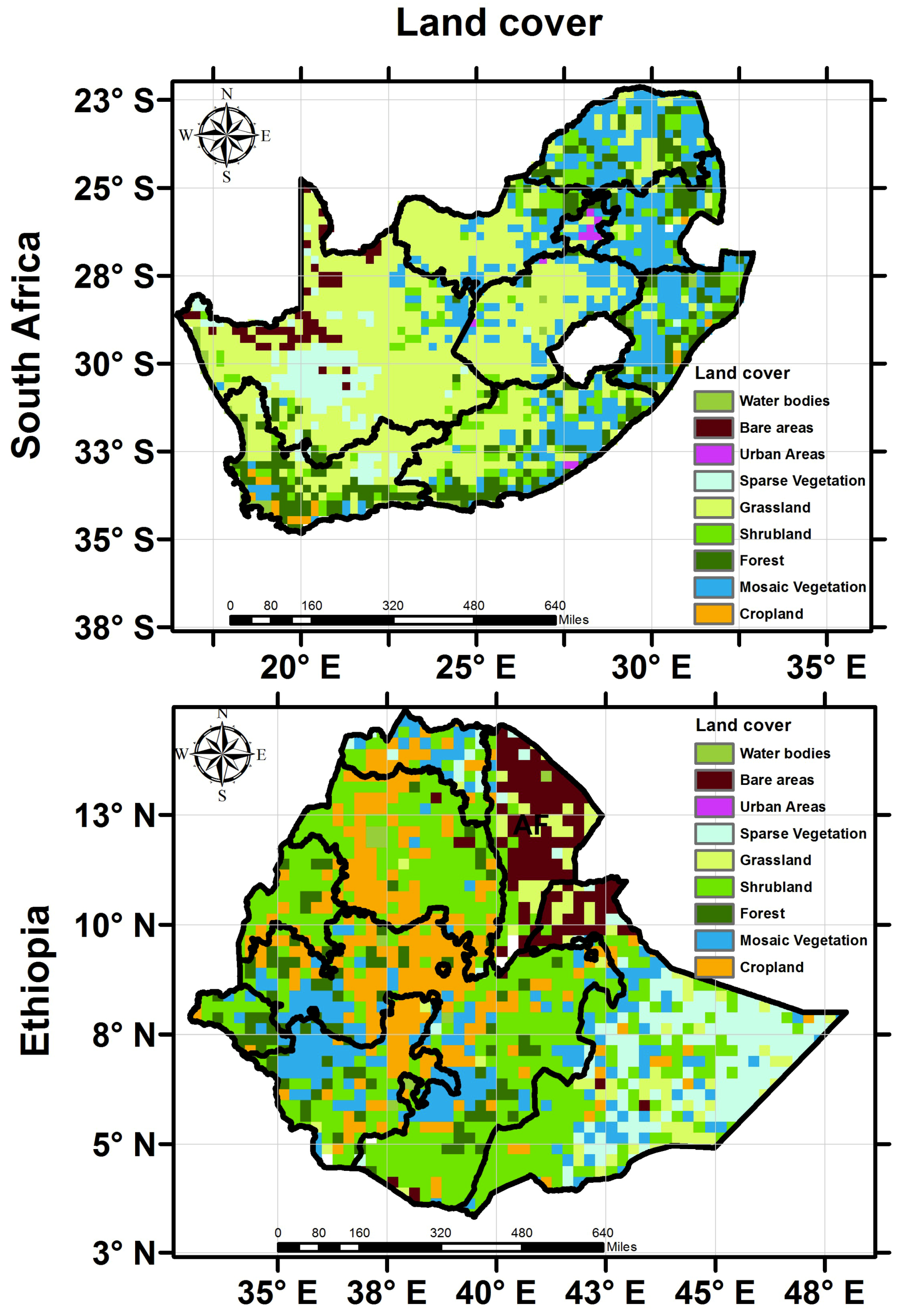
Several additional datasets have been used in this study to explore the relationship between RZSM anomalies and meteorological drought indices as a function of land cover variability. The Climate Hazards Group Infrared Precipitation with Station (CHIRPS) dataset, developed by the United States Geological Survey in collaboration with the Earth Resource Observation and Science center, is used to explore the spatial and temporal variability of precipitation with different land cover types. CHIRPS is generated by integrating satellite imageries and in situ gauge-collected observations. The daily rainfall data are distributed at 0.5° spatial resolution [40]. Vegetation-type information was obtained from the ESA’s global land cover data developed by utilizing observations from the Medium Resolution Imaging Spectrometer collected by the Environmental Satellite [41]. The land cover map includes 22 land cover classes as defined by the Food and Agriculture Organization of the United Nations Land Cover Classification System.
The Standardized Precipitation Index (SPI) is a meteorological drought index used to assess different drought characteristics. It represents the standardized deviation of the observed cumulative precipitation relative to the long-term precipitation average. In this study, SPI at 3-, 6-, and 9-month scales was obtained from the International Research Institute for Climate and Society at Columbia University [21]. The SPI dataset was derived from the Climate Prediction Center’s Outgoing Longwave Radiation blended gauge-based global daily precipitation data. The SPI was calculated by fitting a probability distribution to the long-term series of precipitation accumulation over the period of interest, where the resulting cumulative probability function is consequently transferred to a normal distribution. The monthly SPI data offers global coverage at spatial resolution of 1°.
The Normalized Difference Vegetation Index (NDVI) data were obtained from GIMMS system. This dataset is derived using the Moderate Resolution Imaging Spectroradiometer (MODIS) Terra surface reflectance products, which are provided by NASA Goddard Space Flight Center MODIS Adaptive Processing System [42]. We processed and ingested SPI and NDVI datasets as private assets in the GEE data catalog as those are not available in the GEE public data catalog.
All data products used in this study have been averaged to monthly composites and then resampled to 1° grid spacing to ensure comparable temporal and spatial resolutions among the different datasets.
3. Google Earth Engine Tools
We have developed several GEE tools, which enable easy processing, analysis, and visualization of the SMOS- and SMAP-based soil moisture data in the GEE platform. These tools can be arranged in three groups according to their functionality: (i) tools to process and ingest soil moisture data in the GEE data catalog, (ii) tools to explore spatial and temporal variation of soil moisture and precipitation as a function of land cover, and (iii) tools to estimate drought characteristics such as duration and intensity using soil moisture anomalies and intercomparing the latter against alternative drought indices. Detailed descriptions of the individual tools are given below.
3.1. Data Uploading Routine
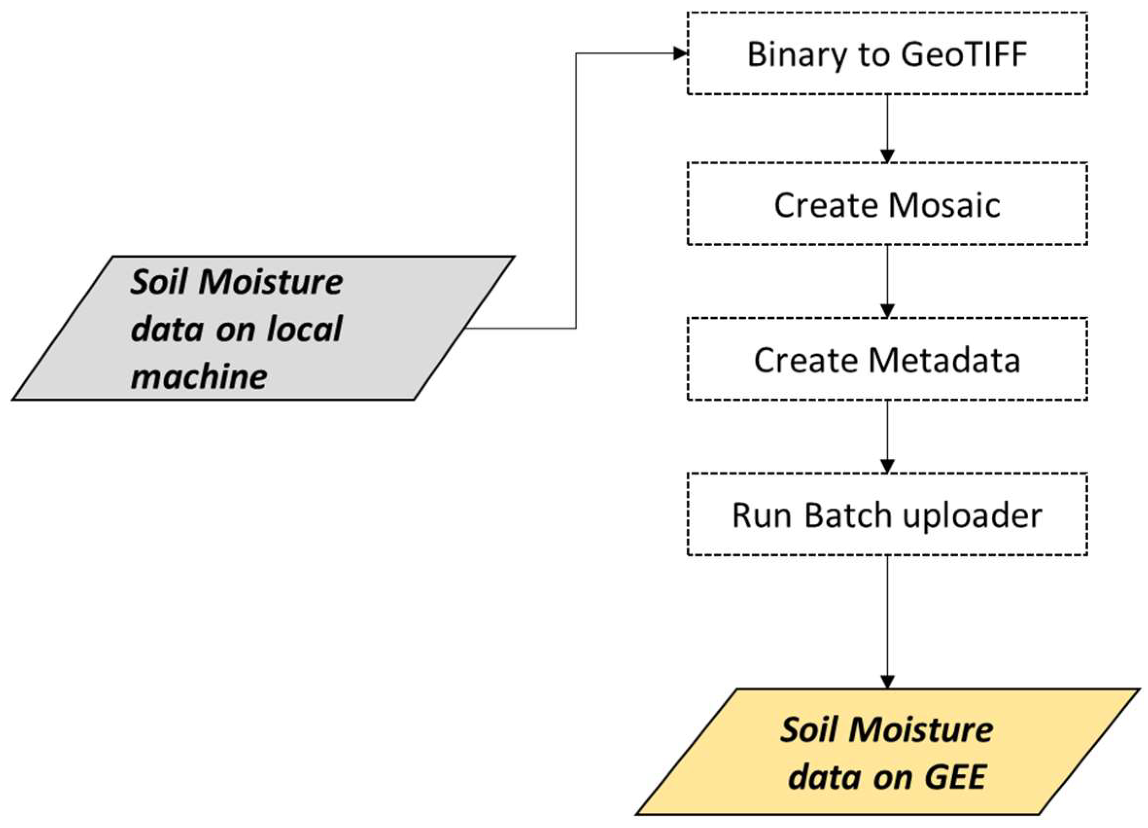
The data upload routine has been designed to process, upload, and manage the SMOS- and SMAP-based soil moisture products in the GEE platform. This routine first converts the original soil moisture data stored in binary format into the georeferenced tagged image file format (GeoTIFF) as required by the GEE. Then, it creates a metadata file of the resulting imagery. The metadata is needed by the analysis routines, which are used to filter the data based on user-specified spatial and temporal information. Next, the GEE batch asset manager (https://github.com/tracek/gee_asset_manager) tool is used to upload a bulk amount of data automatically in the GEE (Figure 2). An alternative uploading option is to use the asset manager option in the GEE. However, the latter is time inefficient for large datasets as it allows the user to upload a single imagery at a time.
3.2. Soil Moisture Exploration Routine
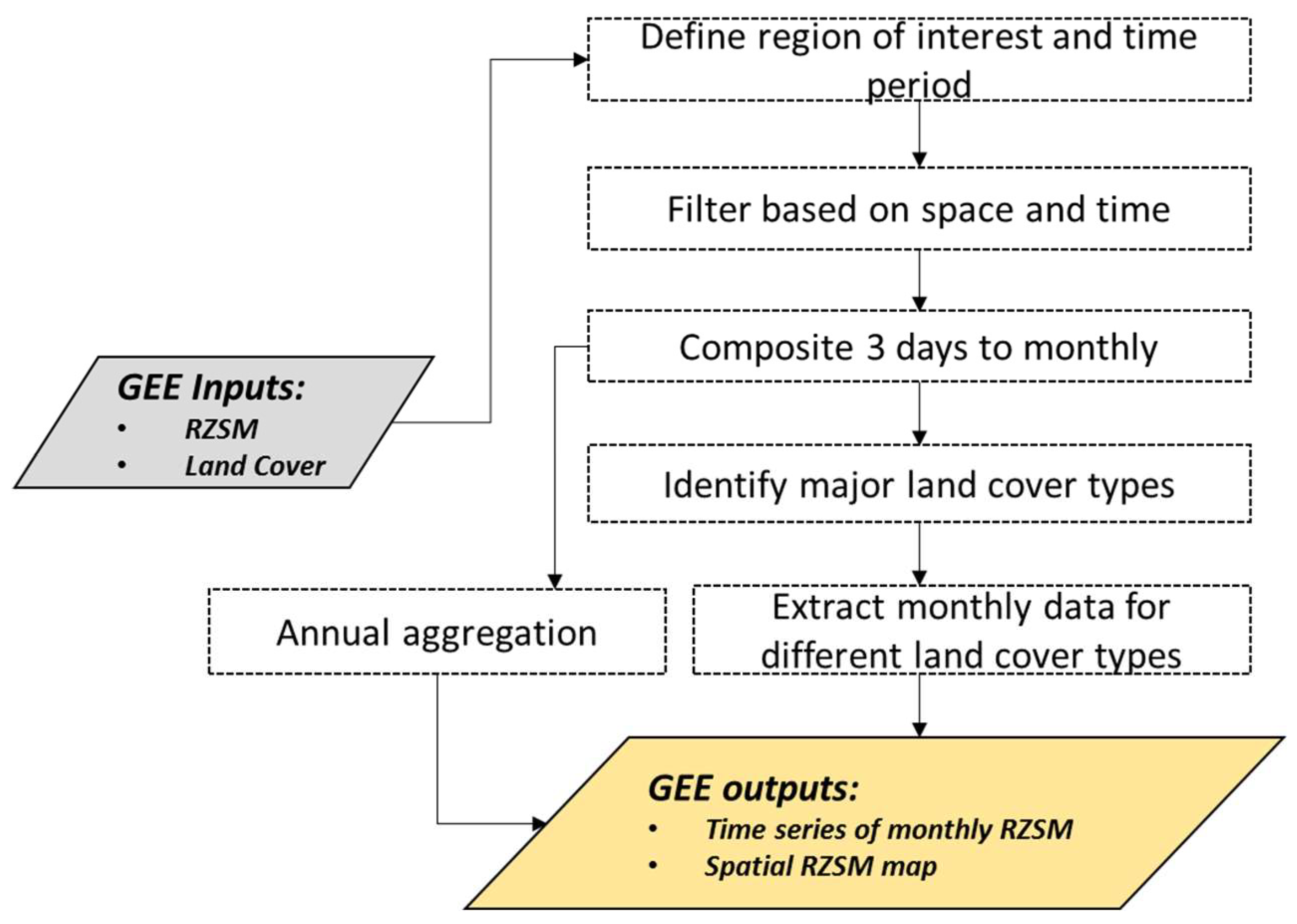
The soil moisture exploration routine has been specifically designed to assess the spatial and temporal variability of soil moisture from local to regional and global scales. This function first filters the soil moisture data based on user-specified temporal and spatial criteria using the GEE ‘filter date’ and ‘filter bounds’ functions. Next, the subset data are grouped by month using the filter calendar range’ function and are aggregated from the original 3-day composites into monthly composites (Figure 3). Then, interactive monthly soil moisture plots are generated using the chart function by using the ‘chart image series’ function in the GEE, which can be viewed and exported in multiple formats (i.e., comma-separated values, portable network graphics, etc.). The multi-annual image collection can be further reduced to a long-term average image representing mean soil moisture for the region of interest, which can be visualized through GEE Google Maps. This routine also enables an assessment of the variability of soil moisture data as a function of land cover type. The ESA land cover data is clipped based on the user-defined region of interest, and a histogram is plotted to estimate the major land cover types of the study region. Then, the monthly soil moisture values are filtered based on land cover class, and interactive plots are generated for additional analysis and visualization.
3.3. Drought Assessment Routine
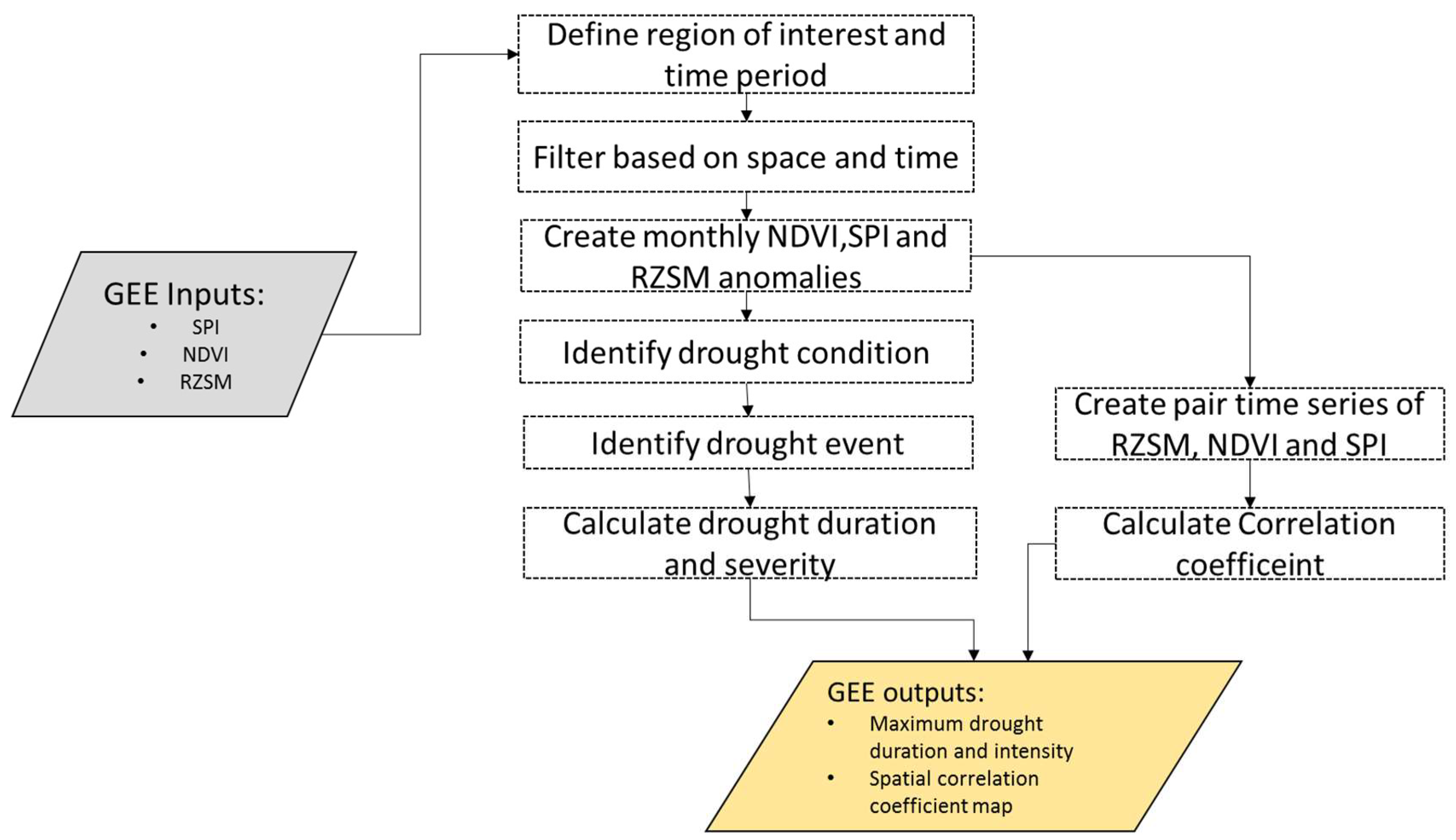
The drought assessment routine has been developed using the GEE functionalities to compare various drought indicators based on specific drought characteristics, such as percentage of the month with drought conditions, maximum drought duration, drought severity, and intensity. In addition, any drought indicators have been developed to monitor, predict, and assess the severity of different drought types, which can be classified into two major categories of drought: meteorological and agricultural. Meteorological drought indicators are derived using precipitation data and have multi-scale features that identify different types of drought condition. As root zone soil moisture affects plant growth and productivity, RZSM anomalies are often used for quantifying and monitoring agricultural drought and capturing its impact on crop heath [4,43,44,45]. In this study, we used four drought indicators—SPI3, SPI6, SPI9 (meteorological drought indicators), and SMOS RZSM anomalies (agricultural drought indicator)—to assess drought conditions. Here, we focused on SMOS RZSM anomalies, as it has longer observation period compared with SMAP and is hence well suited to estimate drought characteristics and Pearson’s correlation coefficient. Positive values of RZSM anomalies, SPI3, SPI6, and SPI9 are masked out to identify only months with drought conditions, the corresponding number is divided by the total number of months to calculate the percentage of months with drought conditions. Each product has been examined in terms of the following drought characteristics: drought duration (defined as the period during which the drought indices are continuously negative); drought severity (computed as the absolute value of the sum of all drought indices during a drought event); and drought intensity (calculated by dividing the severity by the drought duration) [46,47]. This routine also computes cross-correlations between agricultural- and meteorological-based drought indices and allows us to estimate the Pearson, Spearman, and lag correlation coefficients using the GEE ‘reducerpearsonscorrelation’ function between the paired monthly time series of soil moisture anomalies and SPI, as well soil moisture and NDVI (Figure 4).
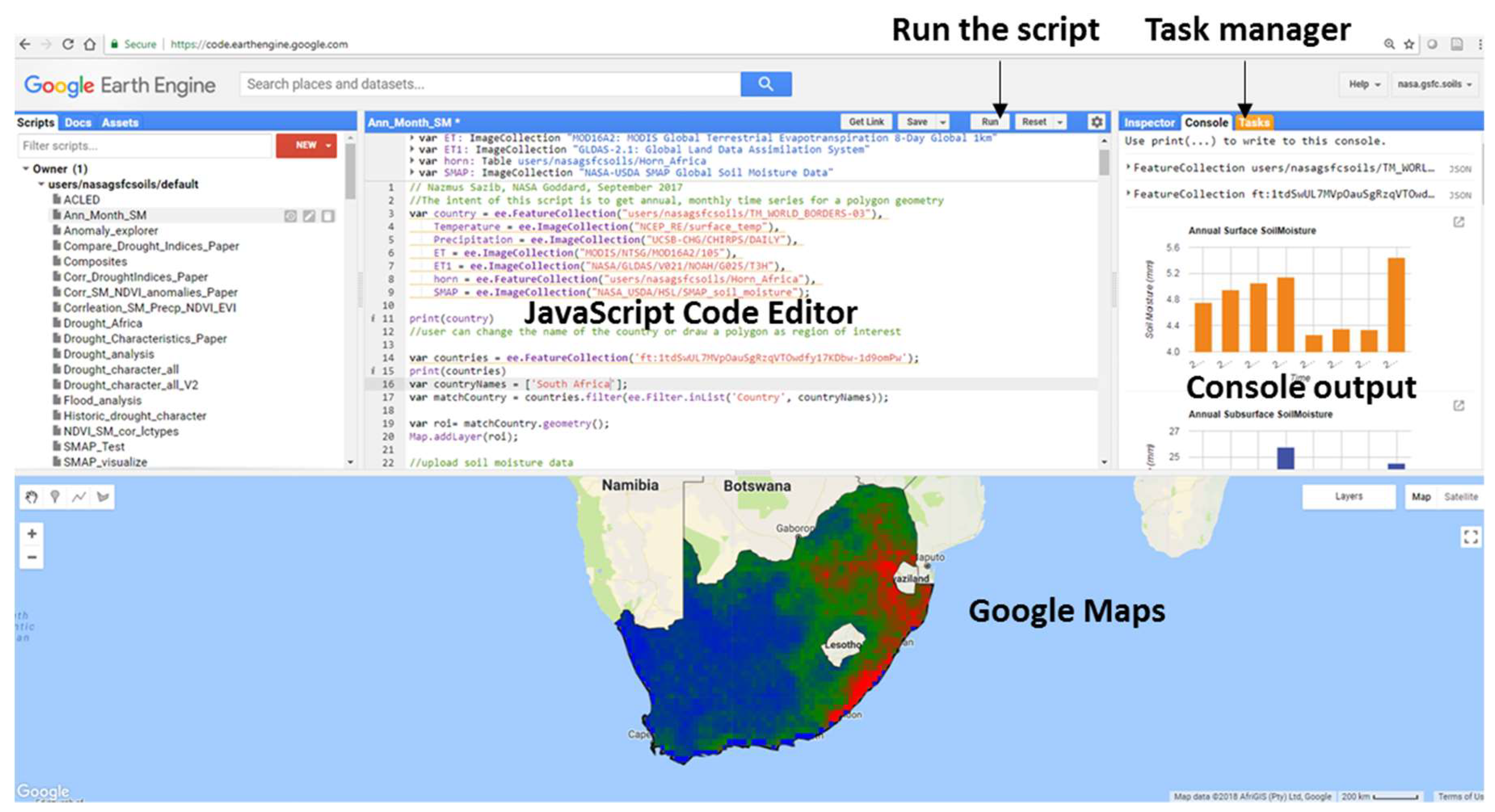
Developed tools are accessible through the links provided in the supplementary materials, though potential users are required to register to access (https://code.earthengine.google.com/). Once the link is clicked, the user is presented with the Google Earth Engine code editor, which is a web-based integrated development environment for the Earth Engine JavaScript Application Programming Interface (Figure 5). Then, the user can execute the program by clicking the ‘run’ button located above the JavaScript code editor panel, if it does not start automatically. Once this has been done, time series plots and a spatial map are displayed in the console tab and Google Maps respectively. The GEE outputs results can be exported by clicking on the run button in the tasks tab located in the right panel next to the code editor.
4. Example Applications
The GEE tools described in the previous section have been implemented to evaluate the spatial and temporal dynamics of soil moisture and precipitation and assess the ability of the drought indices described in the previous sections to capture the severity, duration, and intensity of drought events over South Africa and Ethiopia during 2010–2017.
Drought is common in South Africa and Ethiopia and occurs in all climate areas with varying degrees of intensity, spatial extent, and duration [48]. In recent years, the spatial extent and frequency of drought have increased in this area, causing significant water shortage, economic losses, and adverse social consequences [49]. Therefore, a better understanding of the climatology and drought characteristics over these areas is important in order to improve decision-making and aid activities aimed to mitigate the impact of drought. Our analysis is focused on the 2010–2017-time period, which was determined by the availability of the SMOS datasets. For this analysis, the soil moisture explorer routine is executed in the GEE code editor by clicking on the link provided in the supporting materials to generate spatial map and time series plots of the precipitation and soil moisture over South Africa. Then, we run the drought assessment routine to estimate the drought characteristics and the correlation among the different drought indices over South Africa. Next, we re-run both the soil moisture explorer and the drought assessment routine for Ethiopia by changing the country name inside the script. The output results of the GEE are imported into ArcGIS (Esri, Redlands, CA, USA) [50] to add a legend, scale, and proper color scheme and R [51] to generate boxplots of drought characteristics.
4.1. Spatial and Temporal Variability of Precipitation and Soil Moisture
We first examined the long-term spatial distribution of the precipitation and RZSM and then analyzed the variability of those variables with different land cover types. Spatial variability of rainfall and RZSM over South Africa and Ethiopia are shown in Figure 6. Both variables exhibit high regional variability. In South Africa, generally the mean annual precipitation increases from west to east with the maximum rainfall (680 mm) occurring over the Mpumalanga and KwaZulu-Natal provinces, while minimum rainfall (172 mm) falls over the western part of the country. The spatial variability captured by the RZSM reflects the precipitation variability showing wetter SM conditions in the east and drier conditions in the west (Figure 6, top row). The topographical variability significantly influences the spatial distribution of the precipitation and the soil moisture in Ethiopia. For example, the rainfall and soil moisture values are higher over the highland areas located in the central and northwestern portion of the country, while the lowland areas located in the eastern part of the country are associated with lower rainfall amounts (Figure 6, bottom row).
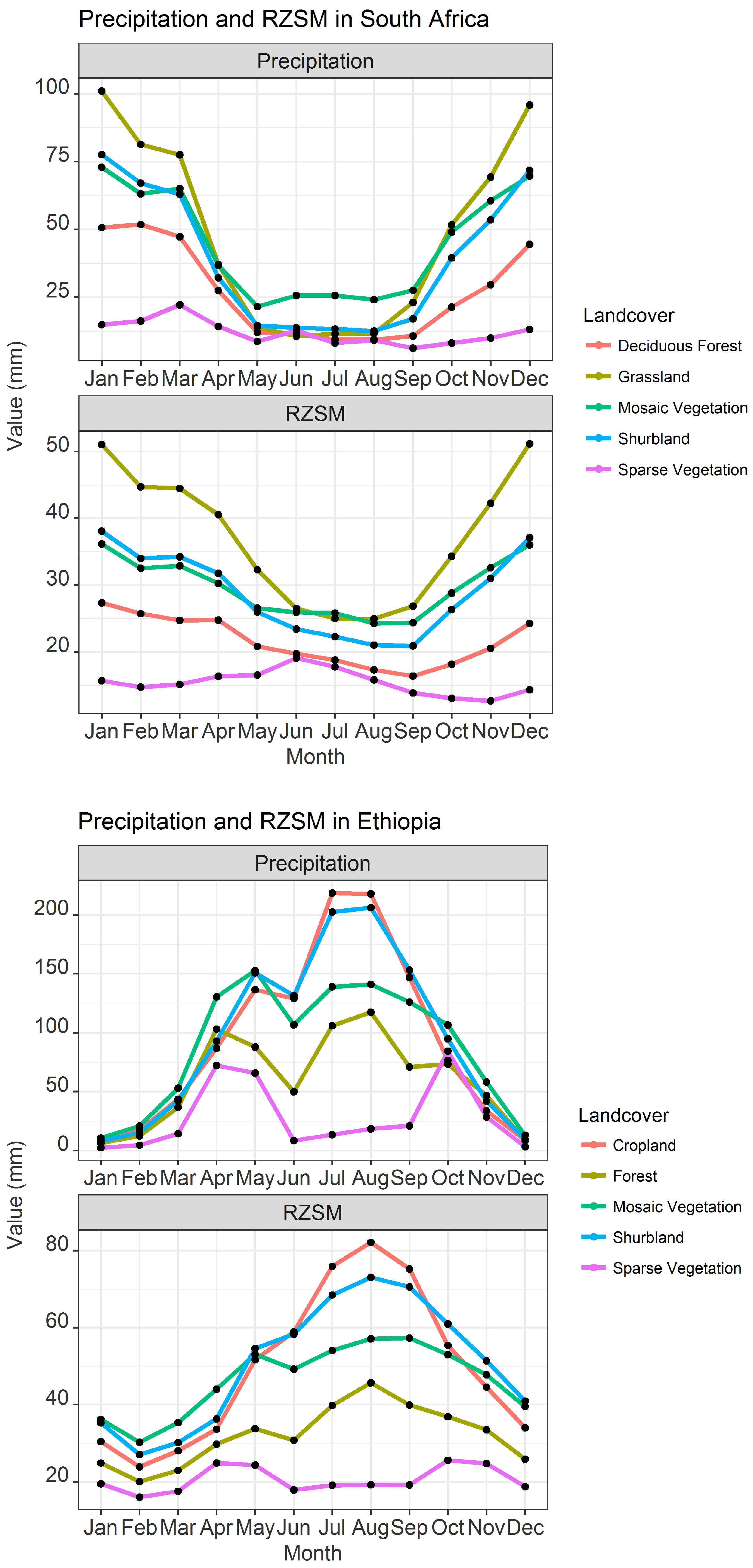
The monthly precipitation over Ethiopia and South Africa is driven mainly by the position of the intertropical convergence zone (ITCZ), which changes over the course of year [52,53]. A majority of the rainfall in Ethiopia falls during the summer seasons when the ITCZ is at its most northern position; however, the amount of rainfall also varies as a function of land cover (Figure 7). For example, forest, cropland, grassland, and shrub land show identical rainfall patterns with one main wet season (June–September) and a secondary wet season (February–May), where the highest rainfall occurs during the month of September (Figure 8). Over sparse vegetation, the major rainfall falls during the summer and winter season, as most of this land cover is located in the southern part of the country, where the rainfall timing is associated with ITCZ, which passes through the southern position of the equator at that time. The monthly RZSM follows the rainfall distribution reaching the wettest soil moisture conditions during the month of September. The position of ITCZ also results in two distinct seasons in South Africa—a wet and dry season roughly from November–April and May–October, respectively. The monthly soil moisture time series captures this seasonality, as seen in Figure 2. The monthly rainfall and soil moisture time series across South Africa vary with land cover, where regions covered by the grassland and sparse vegetation receive the highest and lowest amount of precipitation and soil moisture, respectively (Figure 8).
4.2. Comparison of Drought Characteristics
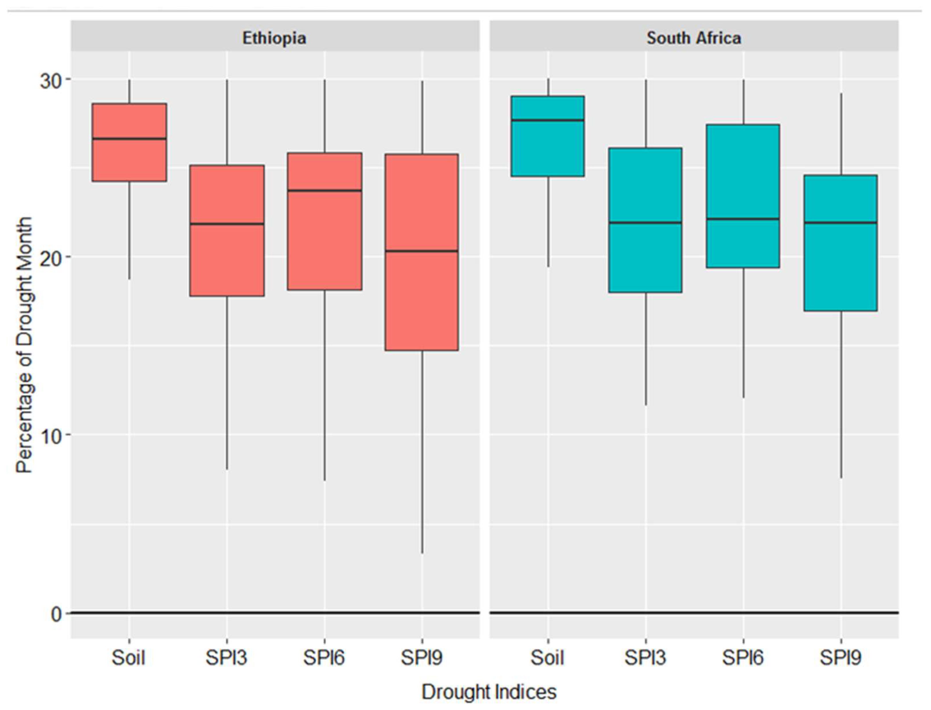
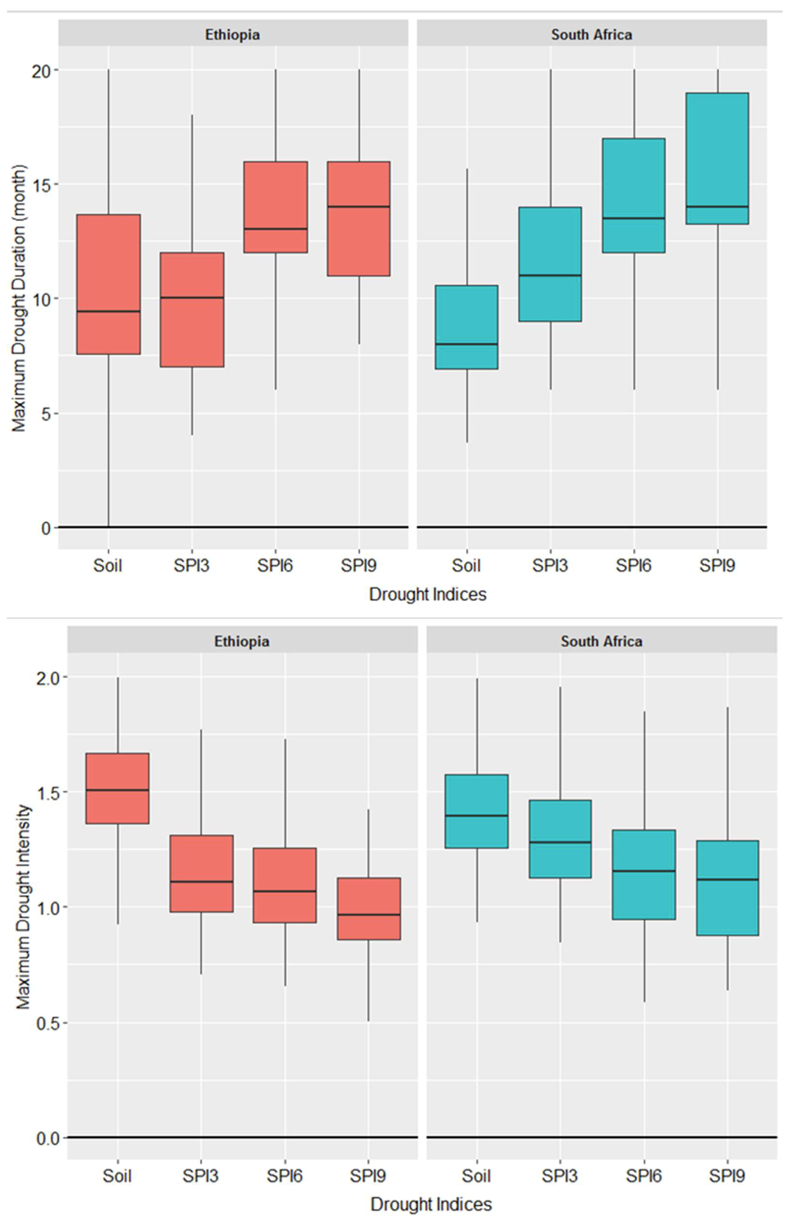
The RZSM anomalies indicated a higher percentage of months with drought conditions compared with SPI (SPI3, SPI6, and SPI9) over both study regions (Figure 9). Over South Africa, the average percentage of drought events identified in the RZSM anomaly data was 27%, which is 6% higher than the drought events captured by the SPI3. Additionally, among the rainfall-based drought indices, the SPI9 had the lowest percentage of months with drought events compared with the SPI3 and SPI6. This is in line with other studies [46], where the author found that agricultural-based drought indicators depict relatively larger values of drought months compared with the meteorological drought indices. The maximum drought duration varied among the different drought indicators. Based on our analysis, the maximum drought duration appeared to be higher in the meteorological-based indices than the agricultural-based indices. This is primarily because the meteorological-based drought indices integrate the drought condition over a longer period of time than do the agricultural-based drought indices [46]. The drought intensity was found to be higher in the agricultural-based drought variables and lower in the metrological-based drought indices. This example demonstrates the capability of the drought assessment tools, which can help to better assess the drought conditions.
4.3. Correlation between Soil Moisture and Normalized Difference Vegetation Index Anomalies
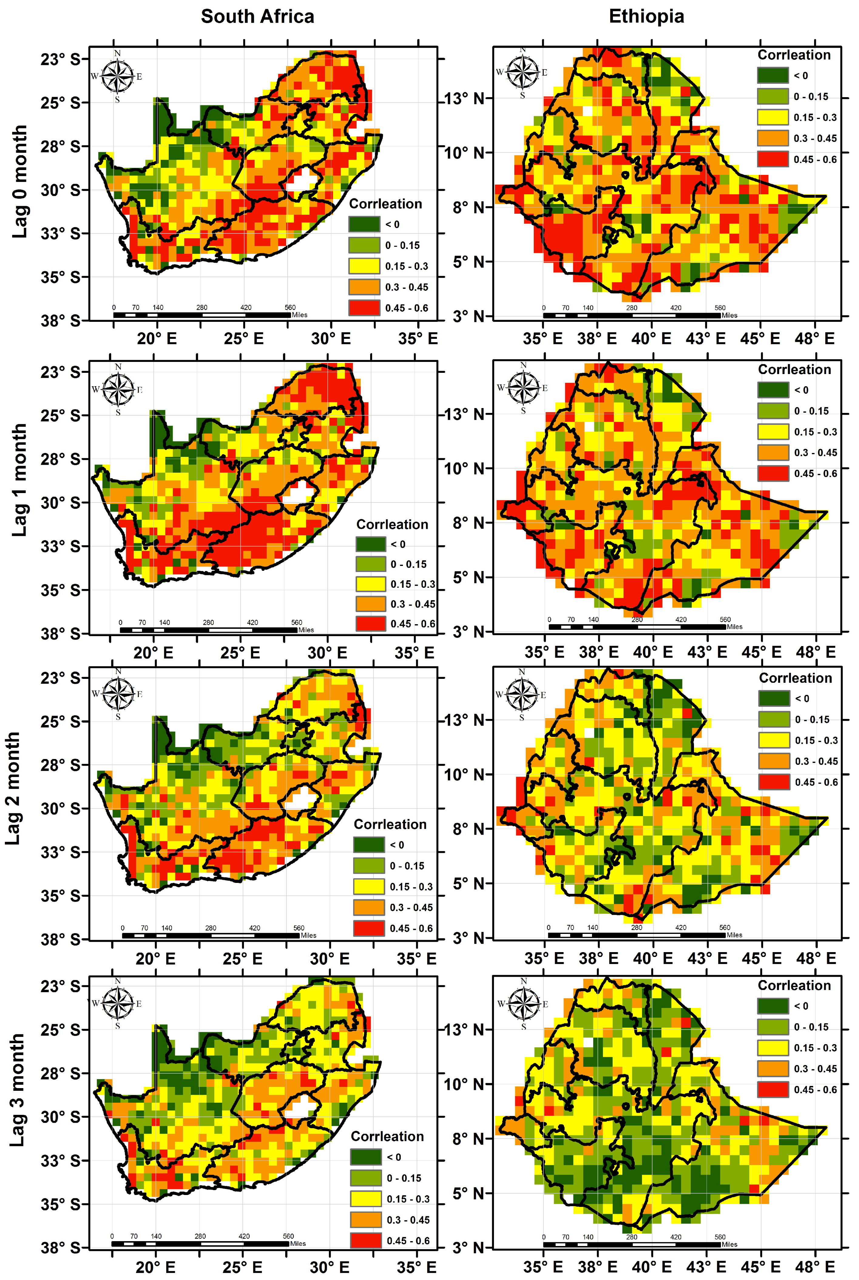
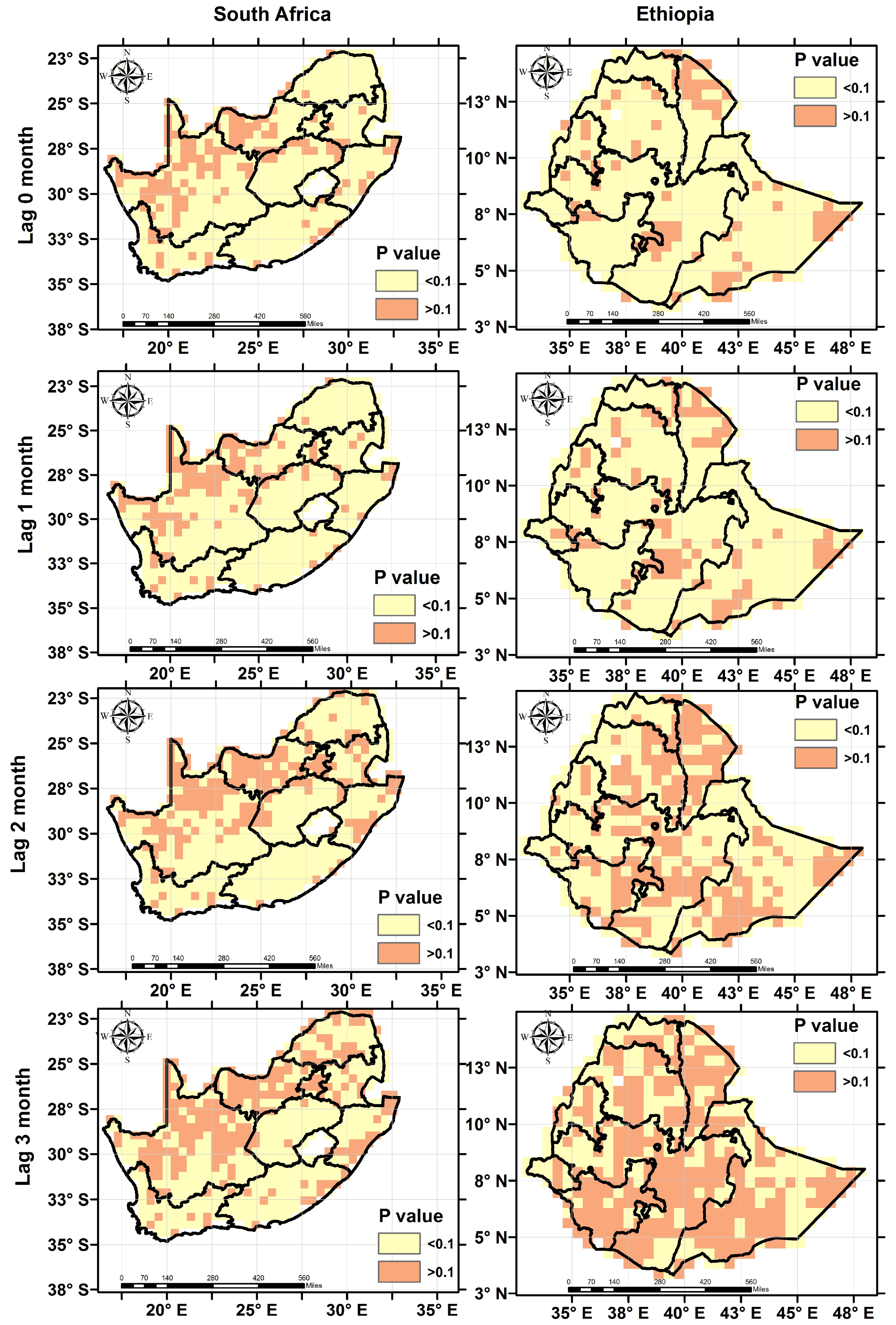
Variations in RZSM substantially influence the vegetation dynamics (i.e., NDVI), which is a widely used vegetation index. Therefore, correlation analysis between RZSM and NDVI anomalies is important to understand the impact of changes in soil moisture on vegetation growth, which can be effectively utilized for early warning of time and areas of increased food insecurity [40,54]. The correlation of the RZSM and NDVI anomalies varied with the geographic location and the degree of lag time. The highest positive correlation coefficients and confidence level (i.e., p-value < 0.1) are observed when soil moisture change is concurrent or precedes the change in NDVI by one month. In most of the locations, NDVI and RZSM anomalies have positive correlations; however, some regions indicate negative correlation at higher lags due to coincidence of negative NDVI anomalies with positive soil moisture anomalies [55]. In South Africa, the semi-arid Western Cape and Eastern Cape show higher coefficients compared with other parts of the country as the vegetation growth in those regions has high reliance on root zone soil moisture [56,57]. No spatial variability in the lag correlation values was observed over Ethiopia (Figure 10). We further investigated the variation of the soil moisture and NDVI relationship as a function of major land cover types. The highest agreement was found over areas covered by grassland for both study areas, while the lowest agreement was achieved over the shrub-covered areas in Ethiopia and South Africa (Table 2). This is partly due to the fact that grassland roots are located on the shallow depths and are more sensitive to changes in soil moisture than deep rooted plants such as shrubs.
4.4. Correlation among Soil Moisture Anomalies and Meteorological Based Indices
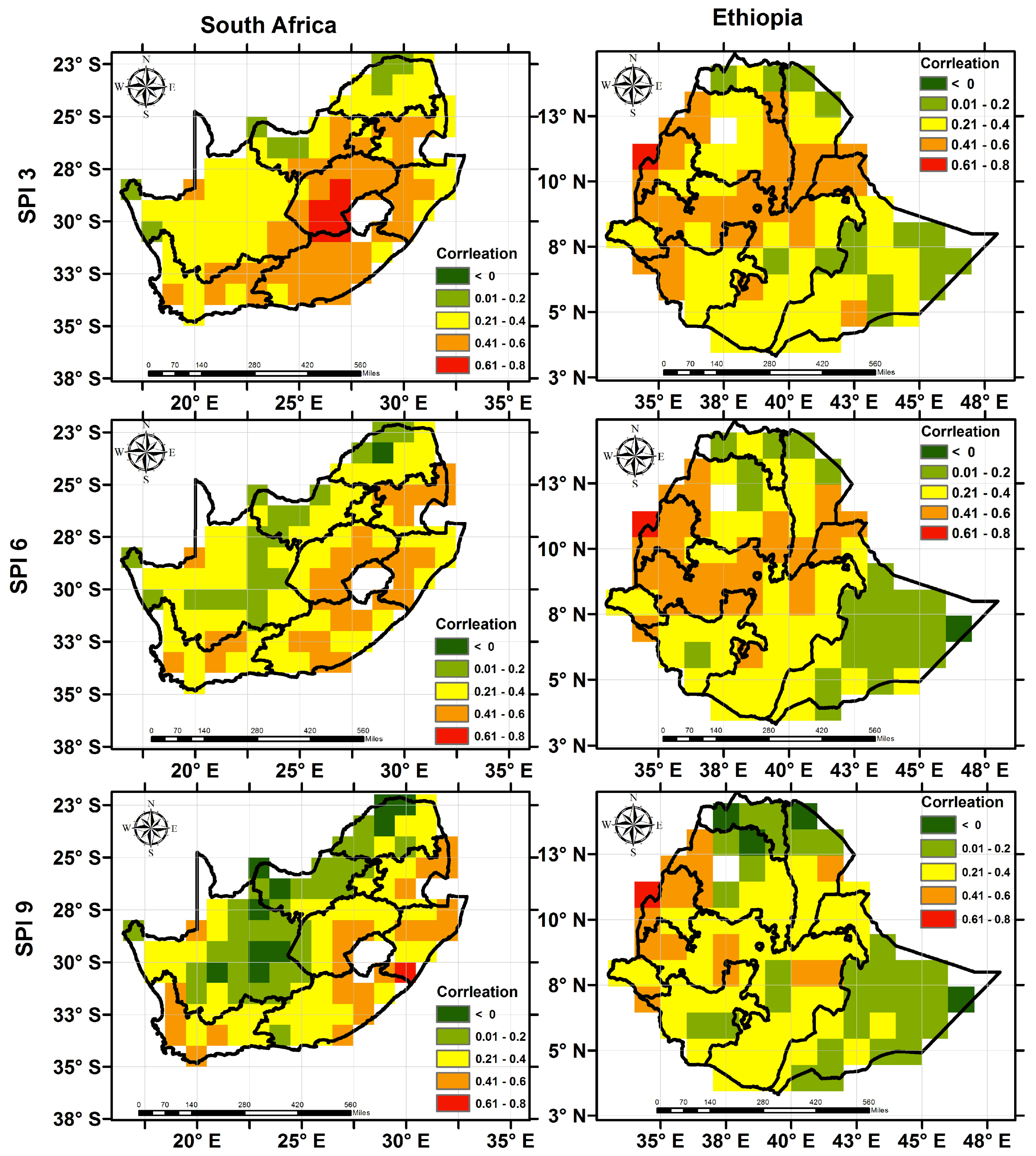
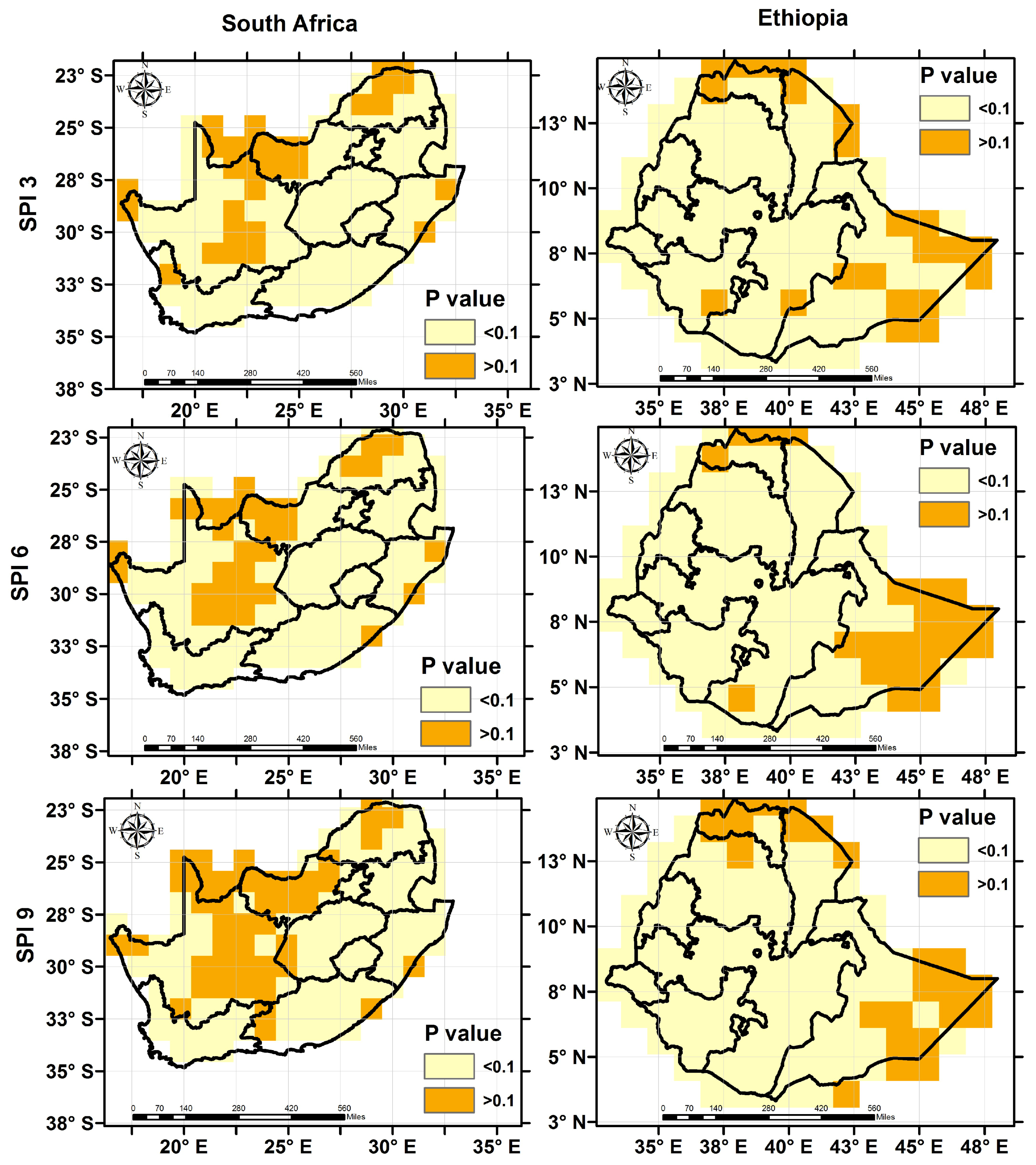
A correlation analysis was carried out between RZSM anomalies and meteorological-based drought indicators to evaluate how well the meteorological-based drought indicators represent agricultural-based drought. Such information could be used to help indicate times and areas that are likely to experience agricultural stress. It is envisaged that such approaches will improve drought monitoring and early warning systems that rely mostly on meteorological indicators [58]. The GEE-based inter-comparative analysis between soil moisture anomalies against SPI showed high agreement and alludes to the value of combining such datasets to compliment a regional drought assessment that incorporates both meteorological and agricultural drought. Over both study regions, SPI3 had higher correlation values compared with SPI6 and SPI9 (Figure 11), which indicates that SPI3 captures more of the agricultural drought. The performance of the meteorological drought indices varied spatially. In the case of South Africa, the correlation values were relatively higher and statistically significant (p-value < 0.1) in the Western Cape and Eastern Cape compared with the Northern Cape of the region. The spatial distribution of the correlation for all meteorological droughts in Ethiopia have similar pattern, where higher and lower correlation values are generally distributed over the northwest and northeast side of the country, respectively. The highest correlation between the soil moisture anomalies and meteorological drought indicators are associated with the cropland (Table 3), which is consistent with [59],who showed that a 3-month SPI has the highest correlation with vegetation growth on croplands of the midlatitude U.S. Great Plains.
5. Discussion
Highest correlation of SPI3 with the RZSM anomalies indicated that short-time meteorological drought represents the agricultural drought better compare with long-term meteorological-based indicators such as SPI6 and SPI9. The impact of meteorological drought on vegetation is cumulative, meaning that vegetation does not respond instantaneously to the precipitation changes. The three-month SPI, which captures the precipitation pattern not only for the specific month of the interest, but also the previous two months, results in a highest correlation between SPI and soil moisture anomalies. On the contrary, the 12- and 6-month SPI values reflect precipitation patterns for annual and the entire growing season, respectively, and tend to diminish the variance in the precipitation data and smooth the SPI values results in lower correlation values [59]. The relationship between soil moisture and rainfall anomalies were also explored by Sims et al. [60] in North Carolina, where the authors suggest that SPI on a scale of 2–3 months yielded the highest correlation with soil moisture anomalies.
Our results indicate lower and higher correlation between RZSM anomalies and SPI-based indicators in the dry and wet regions, respectively, which could be related to the rainfall amount and soil types. The dominant soil types in the wet regions are clay and clay loam, which have higher water-holding capacities, which could result in slower response to the rainfall; therefore, soil moisture on a specific month would be more dependent on the previous month’s rainfall. On the other hand, the arid region shows quicker response to the rainfall anomalies due to dry soil conditions and the limited water-holding capacity of the sandy soils that cover that region. Therefore, soil moisture in a specific month has a smaller dependence on previous months compared with the wet region [61].
In general, the land cover type has a significant impact on the relationship between RZSM anomalies and other drought indicators. For example, shrubland exhibits lower correlation values compared to the cropland, which could be due to the fact that cropland roots are located in the shallow depths and are more sensitive to changes in soil moisture than deep-rooted plants such as shrubs. Similar observations were made by Camberlin et al. [62] and Huber et al. [63] for Africa, by Li et al. [59] for China, and by Wang et al. [60] for the US central Great Plains. We also noticed a delayed response of NDVI to RZSM anomalies for the shrubland over South Africa, which might be related to soil texture and soil moisture amounts, as most of the shrubland is located in the wet region of the country characterized by more clay soils leading to slower response [64]. This is consistent with the findings of Wang et al. [65], who showed that the NDVI at humid sites takes a longer time to respond compared with the arid sites.
6. Conclusions
Soil moisture data are recognized as a fundamental physical variable that can be used to address science and resource-management questions requiring near real-time monitoring of the land–atmosphere boundary, including flood and drought monitoring and regional crop yield assessment. This study introduced new sets of near real-time global soil moisture data and demonstrates the potential of the GEE web-based tools and soil moisture data to assess regional drought conditions. In general, the meteorological drought indicator, SPI3, gives higher correlation values compared with SPI6 and SPI 9 and compared with the RZSM anomalies. When comparing the drought characteristics, RZSM anomalies exhibit relatively larger drought duration but smaller drought intensity compared with the meteorological-based drought indicators. The NDVI-RZSM anomalies are influenced by the vegetation cover, specifically shallow-rooted plants that are more sensitive to soil moisture changes compared with deep-rooted plants. The methods demonstrated here can be applied to other areas requiring early warning of food shortage or improved agricultural monitoring to help provide greater economic security within the agriculture sector.
Incorporating the global soil moisture data into the GEE data catalog enables users to efficiently and quickly acquire and process large amount of data. The available tools allow easy analysis, visualization, and interpretation of the data. To this end, these the GEE-based tools could enable scientists, policy makers, and the general public to explore spatial and temporal variation of soil moisture information and drought conditions for any location in the world with minimal data processing or data management. In addition, all the tools are easily transferable and can be used to explore spatial and temporal dynamics of other climate variables such as temperature and evapotranspiration. The GEE does not require any additional software installation, which helps to overcome compatibility limitations and allows user to access the available codes and data from any computer connected to the internet. This significantly increases the data and tools usability and applicability. The GEE tools and the soil moisture data are open source and are freely available, which can enable users to use, modify, and suggest future improvements for both the tools and the data.
Although the GEE offers many benefits, it has limitations as well. First, it requires basic knowledge of Python and JavaScript, and users with limited programming knowledge might have a steep learning curve. Second, users are sometimes required to export the analyzed results to perform additional analyses due to limited functionalities and plotting options in the GEE. Finally, debugging the code is challenging as the user-created algorithms run in the Google cloud distributed over many computers. Despite these limitations, the data distribution and processing approach offered by the GEE platform can be very beneficial, specifically for developing countries that are typically data-poor areas and lack high-performance data processing platforms for drought monitoring or crop forecasting.
Supplementary Materials
The SMOS and SMAP soil moisture data sets are available at https://explorer.earthengine.google.com/#detail/NASA_USDA%2FHSL%2Fsoil_moisture and https://explorer.earthengine.google.com/#detail/NASA_USDA%2FHSL%2FSMAP_soil_moisture respectively. The soil moisture exploration routine and drought assessment routine are available at https://code.earthengine.google.com/737906c2e5f814170e802859dbe94692, https://code.earthengine.google.com/1da21ee96e5f9ce92a076fc9784485bc and https://code.earthengine.google.com/074dad2e2ddcf24036b2dc0504363281.
Author Contributions
N.S., I.M., and J.B. designed the work. N.S. and I.M. undertook the data analysis. All the authors contributed equally to the final version of the paper.
Funding
This work is supported by the NASA Applied Sciences Program.
Acknowledgments
We would like to thank Simon Ilyushchenko for his support in adding our soil moisture data sets into the Google Earth Engine Public data catalog.
Conflicts of Interest
The authors declare no conflict of interest.
References
- Tsang, L.; Jackson, T. Satellite Remote Sensing Missions for Monitoring Water, Carbon, and Global Climate Change [Scanning the Issue]. Proc. IEEE 2010, 98, 645–648. [Google Scholar] [CrossRef] [Green Version]
- Mladenova, I.E.; Jackson, T.J.; Njoku, E.; Bindlish, R.; Chan, S.; Cosh, M.H.; Holmes, T.R.H.; de Jeu, R.A.M.; Jones, L.; Kimball, J.; et al. Remote monitoring of soil moisture using passive microwave-based techniques—Theoretical basis and overview of selected algorithms for AMSR-E. Remote Sens. Environ. 2014, 144, 197–213. [Google Scholar] [CrossRef]
- McCabe, M.F.; Rodell, M.; Alsdorf, D.E.; Miralles, D.G.; Uijlenhoet, R.; Wagner, W.; Lucieer, A.; Houborg, R.; Verhoest, N.E.C.; Franz, T.E.; et al. The future of Earth observation in hydrology. Hydrol. Earth Syst. Sci. 2017, 21, 3879–3914. [Google Scholar] [CrossRef] [Green Version]
- Eswar, R.; Das, N.N.; Poulsen, C.; Behrangi, A.; Swigart, J.; Svoboda, M.; Entekhabi, D.; Yueh, S.; Doorn, B.; Entin, J. SMAP Soil Moisture Change as an Indicator of Drought Conditions. Remote Sens. 2018, 10, 788. [Google Scholar]
- Blyth, E.M.; Daamen, C.C. The accuracy of simple soil water models in climate forecasting. Hydrol. Earth Syst. Sci. 1997, 1, 241–248. [Google Scholar] [CrossRef] [Green Version]
- Chakraborty, R.; Rahmoune, R.; Ferrazzoli, P. Use of passive microwave signatures to detect and monitor flooding events in Sundarban Delta. In Proceedings of the 2011 IEEE International Geoscience and Remote Sensing Symposium (IGARSS), Vancouver, BC, Canada, 24–29 July 2011; pp. 3066–3069. [Google Scholar]
- Bourgeau-Chavez, L.L.; Kasischke, E.S.; Rutherford, M.D. Evaluation of ERS SAR data for prediction of fire danger in a Boreal region. Int. J. Wildland Fire 1999, 9, 183–194. [Google Scholar] [CrossRef]
- Reichle, R.; Koster, R.D. Global assimilation of satellite surface soil moisture retrievals into the NASA catchment land surface model. Geophys. Res. Lett. 2005, 32, 2353–2364. [Google Scholar] [CrossRef]
- Crow, W.T.; Zhan, X. Continental-Scale Evaluation of Remotely Sensed Soil Moisture Products. IEEE Geosci. Remote Sens. Lett. 2007, 4, 451–455. [Google Scholar] [CrossRef]
- Palmer, W.C. Meteorological Drought; U.S. Weather Bureau Research Paper 45; Office of Climatology, US Department of Commerce: Washington, DC, USA, 1965.
- Bolten, J.D.; Crow, W.T. Improved prediction of quasi-global vegetation conditions using remotely-sensed surface soil moisture. Geophys. Res. Lett. 2012, 39, L19406. [Google Scholar] [CrossRef]
- Bolten, J.D.; Crow, W.T.; Zhan, X.; Jackson, T.J.; Reynolds, C.A. Evaluating the Utility of Remotely Sensed Soil Moisture Retrievals for Operational Agricultural Drought Monitoring. IEEE J. Sel. Top. Appl. Earth Obs. Remote Sens. 2010, 3, 57–66. [Google Scholar] [CrossRef] [Green Version]
- Kerr, Y.H. Soil Moisture and Ocean Salinity SMOS; The European Space Agency: Paris, France, 1998. [Google Scholar]
- Entekhabi, D.; Njoku, E.G.; O’Neill, P.E.; Kellogg, K.H.; Crow, W.T.; Edelstein, W.N.; Entin, J.K.; Goodman, S.D.; Jackson, T.J.; Johnson, J. The Soil Moisture Active Passive (SMAP) Mission. Proc. IEEE 2010, 98, 704–716. [Google Scholar] [CrossRef]
- Gorelick, N.; Hancher, M.; Dixon, M.; Ilyushchenko, S.; Thau, D.; Moore, R. Google Earth Engine: Planetary-scale geospatial analysis for everyone. Remote Sens. Environ. 2017, 202, 18–27. [Google Scholar] [CrossRef]
- Dong, J.; Xiao, X.; Menarguez, M.A.; Zhang, G.; Qin, Y.; Thau, D.; Biradar, C.; Moore, B. Mapping paddy rice planting area in northeastern Asia with Landsat 8 images, phenology-based algorithm and Google Earth Engine. Remote Sens. Environ. 2016, 185, 142–154. [Google Scholar] [CrossRef] [PubMed] [Green Version]
- Boken, V.K.; Cracknell, A.P.; Heathcote, R.L. Monitoring and Predicting Agricultural Drought: A Global Study; Oxford University Press: Oxford, UK, 2005; p. 495. [Google Scholar]
- Lobell, D.B.; Thau, D.; Seifert, C.; Engle, E.; Little, B. A scalable satellite-based crop yield mapper. Remote Sens. Environ. 2015, 164, 324–333. [Google Scholar] [CrossRef]
- NASA-USDA Global Soil Moisture Data. Available online: https://explorer.earthengine.google.com/#detail/NASA_USDA%2FHSL%2Fsoil_moisture (accessed on 10 May 2018).
- NASA-USDA SMAP Global Soil Moisture Data. Available online: https://explorer.earthengine.google.com/#detail/NASA_USDA%2FHSL%2FSMAP_soil_moisture (accessed on 10 May 2018).
- International Research Institute for Climate and Society (IRI). Global Drought Analysis Tool. Available online: https://iridl.ldeo.columbia.edu/maproom/Global/Drought/Global/CPC_GOB/Analysis.html (accessed on 10 May 2018).
- Global Agticultural Monitoring System. Available online: https://glam1.gsfc.nasa.gov/ (accessed on 10 May 2018).
- CHIRPS Pentad: Climate Hazards Group InfraRed Precipitation with Station Data (Version 2.0 Final). Available online: https://explorer.earthengine.google.com/#detail/UCSB-CHG%2FCHIRPS%2FPENTAD. (accessed on 5 May 2018).
- GlobCover: Global Land Cover Map. Available online: https://explorer.earthengine.google.com/#detail/ESA%2FGLOBCOVER_L4_200901_200912_V2_3 (accessed on 5 May 2018).
- Evensen, G. The Ensemble Kalman Filter: Theoretical formulation and practical implementation. Ocean Dyn. 2003, 53, 343–367. [Google Scholar] [CrossRef]
- De Wit, A.J.W.; van Diepen, C.A. Crop model data assimilation with the Ensemble Kalman filter for improving regional crop yield forecasts. Agric. For. Meteorol. 2007, 146, 38–56. [Google Scholar] [CrossRef]
- Crow, W.T.; Kustas, W.P.; Prueger, J.H. Monitoring root-zone soil moisture through the assimilation of a thermal remote sensing-based soil moisture proxy into a water balance model. Remote Sens. Environ. 2008, 112, 1268–1281. [Google Scholar] [CrossRef]
- Reichle, R.H. Data assimilation methods in the Earth sciences. Adv. Water Resour. 2008, 31, 1411–1418. [Google Scholar] [CrossRef]
- Crow, W.; Ryu, D. A new data assimilation approach for improving hydrologic prediction using remotely-sensed soil moisture retrievals. Hydrol. Earth Syst. Sci. 2009, 13, 1–16. [Google Scholar] [CrossRef]
- Panciera, R.; Walker, J.P.; Kalma, J.D.; Kim, E.J.; Saleh, K.; Wigneron, J.-P. Evaluation of the SMOS L-MEB passive microwave soil moisture retrieval algorithm. Remote Sens. Environ. 2009, 113, 435–444. [Google Scholar] [CrossRef]
- Bitar, A.A.; Leroux, D.; Kerr, Y.H.; Merlin, O.; Richaume, P.; Sahoo, A.; Wood, E.F. Evaluation of SMOS Soil Moisture Products Over Continental U.S. Using the SCAN/SNOTEL Network. IEEE Trans. Geosci. Remote Sens. 2012, 50, 1572–1586. [Google Scholar] [CrossRef] [Green Version]
- Jackson, T.J.; Bindlish, R.; Cosh, M.H.; Zhao, T.; Starks, P.J.; Bosch, D.D.; Seyfried, M.; Moran, M.S.; Goodrich, D.C.; Kerr, Y.H.; et al. Validation of Soil Moisture and Ocean Salinity (SMOS) Soil Moisture Over Watershed Networks in the U.S. IEEE Trans. Geosci. Remote Sens. 2012, 50, 1530–1543. [Google Scholar] [CrossRef] [Green Version]
- Van der Schalie, R.; Kerr, Y.H.; Wigneron, J.P.; Rodríguez-Fernández, N.J.; Al-Yaari, A.; de Jeu, R.A. Global SMOS Soil Moisture Retrievals from The Land Parameter Retrieval Model. Int. J. Appl. Earth Obs. Geoinf. 2016, 45, 125–134. [Google Scholar] [CrossRef]
- Chan, S.K.; Bindlish, R.; O’Neill, P.E.; Njoku, E.; Jackson, T.; Colliander, A.; Chen, F.; Burgin, M.; Dunbar, S.; Piepmeier, J.; et al. Assessment of the SMAP Passive Soil Moisture Product. IEEE Trans. Geosci. Remote Sens. 2016, 54, 4994–5007. [Google Scholar] [CrossRef]
- O’Neill, P.E.; Chan, S.; Njoku, E.G.; Jackson, T.J.; Bindlish, R. SMAP Enhanced L2 Radiometer Half-Orbit 9 km EASE-Grid Soil Moisture, Version 1; NASA National Snow and Ice Data Center Distributed Active Archive Center: Boulder, CO, USA, 2016.
- Colliander, A.; Jackson, T.J.; Bindlish, R.; Chan, S.; Das, N.; Kim, S.B.; Cosh, M.H.; Dunbar, R.S.; Dang, L.; Pashaian, L.; et al. Validation of SMAP surface soil moisture products with core validation sites. Remote Sens. Environ. 2017, 191, 215–231. [Google Scholar] [CrossRef]
- Burgin, M.S.; Colliander, A.; Njoku, E.G.; Chan, S.K.; Cabot, F.; Kerr, Y.H.; Bindlish, R.; Jackson, T.J.; Entekhabi, D.; Yueh, S.H. A Comparative Study of the SMAP Passive Soil Moisture Product With Existing Satellite-Based Soil Moisture Products. IEEE Trans. Geosci. Remote Sens. 2017, 55, 2959–2971. [Google Scholar] [CrossRef]
- Al-Yaari, A.; Wigneron, J.P.; Kerr, Y.; Rodriguez-Fernandez, N.; O’Neill, P.E.; Jackson, T.J.; De Lannoy, G.J.M.; Al Bitar, A.; Mialon, A.; Richaume, P. Evaluating soil moisture retrievals from ESA’s SMOS and NASA’s SMAP brightness temperature datasets. Remote Sens. Environ. 2017, 193, 257–273. [Google Scholar] [CrossRef] [PubMed]
- Kumar, S.V.; Peters-Lidard, C.D.; Tian, Y.; Houser, P.R.; Geiger, J.; Olden, S.; Lighty, L.; Eastman, J.L.; Doty, B.; Dirmeyer, P.; et al. Land information system: An interoperable framework for high resolution land surface modeling. Environ. Model. Softw. 2006, 21, 1402–1415. [Google Scholar] [CrossRef]
- Funk, C.; Peterson, P.; Landsfeld, M.; Pedreros, D.; Verdin, J.; Shukla, S.; Husak, G.; Rowland, J.; Harrison, L.; Hoell, A.; et al. The climate hazards infrared precipitation with stations—A new environmental record for monitoring extremes. Sci. Data 2015, 2, 150066. [Google Scholar] [CrossRef] [PubMed]
- Arino, O.; Ramos Perez, J.J.; Kalogirou, V.; Bontemps, S.; Defourny, P.; Van Bogaert, E. Global Land Cover Map for 2009 (GlobCover 2009); European Space Agency (ESA): Paris, France; Université Catholique de Louvain (UCL): Louvain-la-Neuve, Belgium, 2012. [Google Scholar]
- Tucker, C.J.; Pinzon, J.E.; Brown, M.E.; Slayback, D.A.; Pak, E.W.; Mahoney, R.; Vermote, E.F.; El Saleous, N. An extended AVHRR 8-km NDVI dataset compatible with MODIS and SPOT vegetation NDVI data. Int. J. Remote Sens. 2005, 26, 4485–4498. [Google Scholar] [CrossRef]
- Mishra, A.; Vu, T.; Veettil, A.V.; Entekhabi, D. Drought monitoring with soil moisture active passive (SMAP) measurements. J. Hydrol. 2017, 552, 620–632. [Google Scholar] [CrossRef]
- Martínez-Fernández, J.; González-Zamora, A.; Sánchez, N.; Gumuzzio, A. A soil water based index as a suitable agricultural drought indicator. J. Hydrol. 2015, 522, 265–273. [Google Scholar] [CrossRef]
- Hunt Eric, D.; Hubbard Kenneth, G.; Wilhite Donald, A.; Arkebauer Timothy, J.; Dutcher Allen, L. The development and evaluation of a soil moisture index. Int. J. Clim. 2008, 29, 747–759. [Google Scholar] [CrossRef]
- Bayissa, Y.; Maskey, S.; Tadesse, T.; van Andel, J.S.; Moges, S.; van Griensven, A.; Solomatine, D. Comparison of the Performance of Six Drought Indices in Characterizing Historical Drought for the Upper Blue Nile Basin, Ethiopia. Geosciences 2018, 8, 81. [Google Scholar] [CrossRef]
- Tan, C.; Yang, J.; Li, M. Temporal-Spatial Variation of Drought Indicated by SPI and SPEI in Ningxia Hui Autonomous Region, China. Atmosphere 2015, 6, 1399–1421. [Google Scholar] [CrossRef] [Green Version]
- Rouault, M.; Richard, Y. Intensity and spatial extent of droughts in southern Africa. Geophys. Res. Lett. 2005, 32, 297–318. [Google Scholar] [CrossRef]
- Gebrehiwot, T.; van der Veen, A.; Maathuis, B. Spatial and temporal assessment of drought in the Northern highlands of Ethiopia. Int. J. Appl. Earth Obs. Geoinf. 2011, 13, 309–321. [Google Scholar] [CrossRef]
- ESRI 2011. ArcGIS Desktop: Release 10; Environmental Systems Research Institute: Redlands, CA, USA, 2011. [Google Scholar]
- R Core Team. R: A Language and Environment for Statistical Computing; R Foundation for Statistical Computing: Vienna, Austria, 2013. [Google Scholar]
- Jury, M.R. Economic Impacts of Climate Variability in South Africa and Development of Resource Prediction Models. J. Appl. Meteorol. 2002, 41, 46–55. [Google Scholar] [CrossRef]
- Nicholson, S.E. Climate and climatic variability of rainfall over eastern Africa. Rev. Geophys. 2017, 55, 590–635. [Google Scholar] [CrossRef]
- Cash, B.A.; Rodó, X.; Ballester, J.; Bouma, M.J.; Baeza, A.; Dhiman, R.; Pascual, M. Malaria epidemics and the influence of the tropical South Atlantic on the Indian monsoon. Nat. Clim. Chang. 2013, 3, 502. [Google Scholar] [CrossRef]
- Udelhoven, T.; Stellmes, M.; del Barrio, G.; Hill, J. Assessment of rainfall and NDVI anomalies in Spain (1989–1999) using distributed lag models. Int. J. Remote Sens. 2009, 30, 1961–1976. [Google Scholar] [CrossRef]
- Herrmann, S.M.; Anyamba, A.; Tucker, C.J. Recent trends in vegetation dynamics in the African Sahel and their relationship to climate. Glob. Environ. Chang. 2005, 15, 394–404. [Google Scholar] [CrossRef]
- Asoka, A.; Mishra, V. Prediction of vegetation anomalies to improve food security and water management in India. Geophys. Res. Lett. 2015, 42, 5290–5298. [Google Scholar] [CrossRef] [Green Version]
- Bachmair, S.; Tanguy, M.; Hannaford, J.; Stahl, K. How well do meteorological indicators represent agricultural and forest drought across Europe? Environ. Res. Lett. 2018, 13, 034042. [Google Scholar] [CrossRef] [Green Version]
- Ji, L.; Peters, A.J. A spatial regression procedure for evaluating the relationship between AVHRR-NDVI and climate in the northern Great Plains. Int. J. Remote Sens. 2004, 25, 297–311. [Google Scholar] [CrossRef]
- Sims, A.P.; Niyogi, D.D.; Raman, S. Adopting drought indices for estimating soil moisture: A North Carolina case study. Geophys. Res. Lett. 2002, 29, 24-1. [Google Scholar] [CrossRef]
- Richards, J.F. Drought Assessment Tools for Agricultural Water Management in Jamaica; McGill University Library: Montreal, QC, Canada, 2010. [Google Scholar]
- Camberlin, P.; Martiny, N.; Philippon, N.; Richard, Y. Determinants of the interannual relationships between remote sensed photosynthetic activity and rainfall in tropical Africa. Remote Sens. Environ. 2007, 106, 199–216. [Google Scholar] [CrossRef] [Green Version]
- Huber, S.; Fensholt, R.; Rasmussen, K. Water availability as the driver of vegetation dynamics in the African Sahel from 1982 to 2007. Glob. Planet. Chang. 2011, 76, 186–195. [Google Scholar] [CrossRef]
- Jamali, S.; Seaquist, J.; Ardö, J.; Eklundh, L. Investigating temporal relationships between rainfall, soil moisture and MODIS-derived NDVI and EVI for six sites in Africa. In Proceedings of the 34th International Symposium on Remote Sensing of Environment, Sydney, Australia, 21 April 2011. [Google Scholar]
- Wang, J.; Rich, P.M.; Price, K.P. Temporal responses of NDVI to precipitation and temperature in the central Great Plains, USA. Int. J. Remote Sens. 2003, 24, 2345–2364. [Google Scholar] [CrossRef] [Green Version]
Figure 1.
Schematic overview of the methodological approach. SMOS, Soil Moisture Ocean Salinity mission; SMAP, Soil Moisture Active Passive mission; ESA, European Space Agency; CHIRPS; Climate Hazards Group Infrared Precipitation with Station; NDVI, Normalized Difference Vegetation Index; SPI, Standardized Precipitation Index; and RZSM, root zone soil moisture.

Figure 2.
Ingestion of soil moisture datasets to the Google Earth Engine (GEE). The gray and gold boxes represent inputs and outputs, respectively. GeoTIFF, georeferenced tagged image file format.
Figure 2.
Ingestion of soil moisture datasets to the Google Earth Engine (GEE). The gray and gold boxes represent inputs and outputs, respectively. GeoTIFF, georeferenced tagged image file format.

Figure 3.
Data processing steps in the soil moisture exploration routine. The gray and gold boxes represent GEE inputs and outputs, respectively. The boxes identified by dotted lines represent the processes that run in the GEE server.
Figure 3.
Data processing steps in the soil moisture exploration routine. The gray and gold boxes represent GEE inputs and outputs, respectively. The boxes identified by dotted lines represent the processes that run in the GEE server.

Figure 4.
Data processing steps in the drought assessment routine using the GEE. The gray and gold boxes represent GEE inputs and outputs, respectively. The boxes identified by the dotted lines represent the process that run in the GEE server.
Figure 4.
Data processing steps in the drought assessment routine using the GEE. The gray and gold boxes represent GEE inputs and outputs, respectively. The boxes identified by the dotted lines represent the process that run in the GEE server.

Figure 5.
Components of Google Earth Engine code editor.

Figure 6.
Spatial variability of precipitation (derived from CHIRPS precipitation data) and RZSM (derived from United States Department of Agriculture-Foreign Agricultural Services (USDA-FAS) soil moisture data) over South Africa (top row) and Ethiopia (bottom row) for the period of 2010–2017. The locations of the each province of South Africa (NC: Northern Cape, WC: Western Cape, EC: Eastern Cape, NW: North West, FS: Free State, KN: KwaZulu-Natal, MP: Mpumalanga, GA: Gauteng, and LI: Limpopo) and Ethiopia (SO: Somali, OR: Oromia, SN: Southern Nations, GP: Gambela Peoples, BG: Benshangul-Gumaz, AM: Amhara, TI: Tigray, AF: Afar, and AB: Addis Ababa) are also indicated.

Figure 7.
Land cover of South Africa (top) and Ethiopia (bottom).

Figure 8.
Monthly variation of soil moisture and rainfall for different land cover types over South Africa (top) and Ethiopia (bottom).
Figure 8.
Monthly variation of soil moisture and rainfall for different land cover types over South Africa (top) and Ethiopia (bottom).

Figure 9.
Comparison of percentage of months with drought conditions, maximum drought duration, and drought intensity over Ethiopia and South Africa for multiple drought indices. The center line of each boxplot depicts the median value (50th percentile) and the box encompasses the 25th and 75th percentiles of the sample data. The whiskers extend from q1 − 1.5 × (q3 − q1) to q3 + 1.5 × (q3 − q1), where q1 and q3 are the 25th and 75th percentiles of the sample data, respectively.


Figure 10.
Correlation coefficient (top) and p-value (bottom) between RZSM and NDVI anomalies for different lag times.
Figure 10.
Correlation coefficient (top) and p-value (bottom) between RZSM and NDVI anomalies for different lag times.


Figure 11.
Spatial variation of Pearson correlation coefficients (top) and p-value (bottom) of RZSM anomalies with meteorological-based drought indices.
Figure 11.
Spatial variation of Pearson correlation coefficients (top) and p-value (bottom) of RZSM anomalies with meteorological-based drought indices.


Table 1.
Datasets used in this study.
| No | Name | Spatial Resolution | Temporal Resolution | URL |
|---|---|---|---|---|
| 1 | NASA-USDA Global Soil Moisture Data | 0.25° | 3 days | [19] |
| 2 | NASA-USDA SMAP Global Soil Moisture Data | 0.25° | 3 days | [20] |
| 3 | SPI | 1° | monthly | [21] |
| 4 | NDVI | 0.00225° | 8 days | [22] |
| 5 | CHIRPS Pentad: Climate Hazards Group InfraRed Precipitation with Station Data | 0.05° | 5 days | [23] |
| 6 | Global Land Cover Map | 0.00275° | [24] |
NASA, National Aeronautics Space Agency; USDA, United States Department of Agriculture.
Table 2.
The Pearson’s correlation coefficient computed between agricultural-based drought indices and meteorological-based drought indices for different land cover types.
Table 2.
The Pearson’s correlation coefficient computed between agricultural-based drought indices and meteorological-based drought indices for different land cover types.
| Ethiopia | South Africa | |||||||
|---|---|---|---|---|---|---|---|---|
| Land Cover | Lag0 | Lag1 | Lag2 | Lag3 | Lag0 | Lag 1 | Lag2 | Lag 3 |
| Cropland | 0.32 | 0.31 | 0.20 | 0.13 | 0.31 | 0.32 | 0.25 | 0.25 |
| Grassland | 0.34 | 0.32 | 0.21 | 0.11 | 0.37 | 0.38 | 0.28 | 0.23 |
| Shrubland | 0.32 | 0.30 | 0.20 | 0.11 | 0.24 | 0.29 | 0.23 | 0.18 |
Table 3.
The Pearson’s correlation coefficient computed between agricultural-based drought indices and meteorological-based drought indices for different land cover types.
Table 3.
The Pearson’s correlation coefficient computed between agricultural-based drought indices and meteorological-based drought indices for different land cover types.
| Ethiopia | South Africa | |||||
|---|---|---|---|---|---|---|
| Land Cover | SPI3 | SPI6 | SPI9 | SPI3 | SPI6 | SPI9 |
| Cropland | 0.41 | 0.42 | 0.32 | 0.43 | 0.39 | 0.34 |
| Grassland | 0.37 | 0.36 | 0.29 | 0.37 | 0.30 | 0.23 |
| Shrubland | 0.25 | 0.21 | 0.16 | 0.37 | 0.28 | 0.20 |
© 2018 by the authors. Licensee MDPI, Basel, Switzerland. This article is an open access article distributed under the terms and conditions of the Creative Commons Attribution (CC BY) license (http://creativecommons.org/licenses/by/4.0/).
Share and Cite
MDPI and ACS Style
Sazib, N.; Mladenova, I.; Bolten, J. Leveraging the Google Earth Engine for Drought Assessment Using Global Soil Moisture Data. Remote Sens. 2018, 10, 1265. https://doi.org/10.3390/rs10081265
AMA Style
Sazib N, Mladenova I, Bolten J. Leveraging the Google Earth Engine for Drought Assessment Using Global Soil Moisture Data. Remote Sensing. 2018; 10(8):1265. https://doi.org/10.3390/rs10081265
Chicago/Turabian StyleSazib, Nazmus, Iliana Mladenova, and John Bolten. 2018. "Leveraging the Google Earth Engine for Drought Assessment Using Global Soil Moisture Data" Remote Sensing 10, no. 8: 1265. https://doi.org/10.3390/rs10081265
Note that from the first issue of 2016, this journal uses article numbers instead of page numbers. See further details here.