Abstract
Land surface albedo determines the splitting of downwelling solar radiation into components which are either reflected back to the atmosphere or absorbed by the surface. Land surface albedo is an important variable for the climate community, and therefore was defined by the Global Climate Observing System (GCOS) as an Essential Climate Variable (ECV). Within the scope of the Satellite Application Facility for Land Surface Analysis (LSA SAF) of EUMETSAT (European Organization for the Exploitation of Meteorological Satellites), a near-real time (NRT) daily albedo product was developed in the last decade from observations provided by the Spinning Enhanced Visible and Infrared Imager (SEVIRI) instrument on board the geostationary satellites of the Meteosat Second Generation (MSG) series. In this study we present a new collection of albedo satellite products based on the same satellite data. The MSG Ten-day Albedo (MTAL) product incorporates MSG observations over 31 days with a frequency of NRT production of 10 days. The MTAL collection is more dedicated to climate analysis studies compared to the daily albedo that was initially designed for the weather prediction community. For this reason, a homogeneous reprocessing of MTAL was done in 2018 to generate a climate data record (CDR). The resulting product is called MTAL-R and has been made available to the community in addition to the NRT version of the MTAL product which has been available for several years. The retrieval algorithm behind the MTAL products comprises three distinct modules: One for atmospheric correction, one for daily inversion of a semi-empirical model of the bidirectional reflectance distribution function, and one for monthly composition, that also determines surface albedo values. In this study the MTAL-R CDR is compared to ground surface measurements and concomitant albedo products collected by sensors on-board polar-orbiting satellites (SPOT-VGT and MODIS). We show that MTAL-R meets the quality requirements if MODIS or SPOT-VGT are considered as reference. This work leads to 14 years of production of geostationary land surface albedo products with a guaranteed continuity in the LSA SAF for the future years with the forthcoming third generation of European geostationary satellites.
1. Introduction
The monitoring of the climate of our planet has become essential in the current context of climate change [1]. Proper monitoring is impossible without long term and accurate observations of climate variables [2,3]. These long-term observations are nowadays available thanks to the data collected during the past decades by the instruments on board Earth observation satellites. These data time series allow the climate community to study and monitor the underlying Earth’s surface and atmosphere for a long and climatologically relevant period of time. Along with satellite observations, ground stations also contribute to the data collection effort, while they also participate in the validation of the satellite-derived information.
Land surface albedo is an important variable for the climate community. Surface albedo was defined as an Essential Climate Variable (ECV) by the Global Climate Observing System (GCOS), as it stands for the ratio of the radiation reflected from the surface of the Earth to the total incoming radiation. Land surface albedo therefore determines how much radiation is absorbed by the Earth’s land surface and, as a corollary, how much energy is reflected back to the atmosphere. As surface albedo drives the Earth’s energy budget, it gains prominence in numerical weather prediction models and general circulation models [4]. This surface variable is required to understand the phenomena that take place in the lower layers of the atmosphere and to constrain the surface atmosphere coupled models. For example, Crook and Forster [5] observed that the use of satellite observations of surface albedo had a significant impact on the feedback of several ocean atmosphere coupled climate models. Gaining knowledge over the temporal and spatial evolution of surface albedo is key for climate studies, as this ECV is both a forcing variable controlling the climate as well as a sensitive indicator of environmental degradation. Finally, albedo values at different wavelengths contain a wealth of information about the physical state of the surface that can be used for a variety of applications such as vegetation monitoring and land cover classification.
Land surface albedo varies in space and time as a result of natural processes (e.g., changes in solar position, snowfall, vegetation growth) and human activities (e.g., clearing and planting forests, sewing and harvesting crops, burning range land) [6]. The recently observed greening of the vegetation in several regions of the world [7] may be related to observable albedo trends. Also, the monitoring of surface albedo may be used to detect changes of land cover that modify the quantity of energy reflected back to space. In this context spaceborne remote sensing represents a unique tool of measuring and monitoring the global heterogeneity of this ECV at the global scale and in a continuous manner. The observations acquired by sensors on board polar orbiting satellites and geostationary spacecrafts are already helping the scientific community to follow those temporal and spatial evolutions. In particular the highly frequent observations provided by geostationary satellites can be useful over boreal regions in order to track the rapid melt of ice and snow [8]. Furthermore, the study of albedo variations of the vegetation cover needs a time step of no more than one day to be able to detect shifts of about +2/+3 days per decade in the start of the growing season [9,10].
In the last two decades land surface albedo products have been derived from different spaceborne instruments including AVHRR [11,12], POLDER [13], MODIS [14,15], MVIRI [16], AVIRIS [17], VEGETATION [18,19], PROBA-V [20], VIRSS (SNPP/NOAA-20) [20], GOES-R [21], and SEVIRI [22]. And several initiatives as GlobAlbedo [23,24] or GLASS [25] have provided long-term albedo products from these satellite data. Most of these satellite products provide broadband albedo values that result from integrating the surface albedo from 0.3 µm to 4.0 µm. These wavelengths correspond to the solar spectral domain in which the major portion of the energy is found in the visible range. The solar radiation that reaches the surface is previously subject to an attenuation coming from the atmospheric constituents such as water vapor, ozone, and aerosols [26,27]. The accuracy of satellite-derived albedo is dependent on the correction for these effects using atmospheric correction techniques. Other factors impacting the quality of albedo estimates are the field of view of the satellite, calibration errors, the bidirectional reflectance model used in the inversion process, and the spectral-to-broadband albedo conversion [28]. The quality of these products is regularly assessed, and their accuracy is estimated to be around 10% on average [28]. However, the GCOS specified a set of global target requirements with an objective of accuracy of 5%. The reason behind this figure is to provide products accurate enough to detect the change of a radiative forcing equivalent to 20% of the expected total change in radiative forcing per decade due to greenhouse gases and other forcings, i.e., ~0.1 W·m−2 per decade [29].
The Satellite Application Facility on Land Surface Analysis (LSA SAF) is a EUMETSAT (European Organization for the Exploitation of Meteorological Satellites) program [30]. The program aims to retrieve from satellites and disseminate a set of parameters involved in the surface radiation budget, evapotranspiration, vegetation cover and fire-related products (http://lsa-saf.eumetsat.int/). The LSA SAF provides information that is near-real time (NRT), reliable, and up-to-date, on how our planet and its climate are changing. This can help decision makers, businesses, and citizens to define environmental policies and decide mitigation actions [31]. The LSA SAF project is part of the SAF network, a set of specialized development and processing centers, serving as EUMETSAT distributed Applications Ground Segment. The SAF network complements the product-oriented activities at the EUMETSAT Central Facility in Darmstadt, Germany. The main purpose of the LSA SAF is to take full advantage of remotely sensed data over land to measure bio-geophysical variables, which target a wide range of applications, from meteorology and climate to hydrology and agriculture or forest management. The project started in 1999 and entered its third Continuous Development and Operational Phase in March 2017.
The LSA SAF has been especially designed to serve the needs of the NRT meteorological community, particularly for numerical weather prediction (NWP). The LSA SAF also addresses other communities including users interested in climatological applications who require long and homogeneous time series. The delivered satellite products exploit data acquired from the instruments on board the Meteosat Second Generation (MSG) platform and the Meteorological-Operational (Metop) satellites. The product portfolio of the LSA SAF comprises variables such as temperature, short-wave and long-wave downwelling radiation, turbulent fluxes (including evapotranspiration), leaf area index and vegetation cover fraction, and surface albedo. In addition to the NRT production of these biophysical variables, a first long term reprocessed time series (called climate data record, CDR) of several of these biophysical variables (including land surface albedo) was made available to the community in 2018.
CDRs are gaining prominent importance in the field of climate science. They are defined to be a continuous time series of important climate variables, that are relevant for determining the climate variability. CDRs are also found important in several environmental research applications involving agriculture, forestry, hydrology, and energy. They are further used to assess the risk management for envisaging mitigation procedures. In the context of climate variability it is important for the scientific community to understand if the trends associated with time series of geophysical variables are significant and also to assess their uncertainty [32]. This is possible only with the observation and analysis of long term CDRs. Detailed explanation of the CDRs and their importance are found in several studies [33,34]. For example, the CDRs data records of EUMETSAT are used in climate models for the robust estimation of long term surface properties [35].
The objective of this article is to present the new satellite land surface albedo products based on monthly accumulated MSG observations and developed in the LSA SAF project. Two collections exist: An NRT product (named MSG Ten-day Albedo, MTAL), and a reprocessing or CDR from 2004 (named reprocessed MTAL, MTAL-R). The two collections are generated with the same retrieval algorithm but with slightly different input data. After presenting the retrieval method this article focuses on the assessment of the surface albedo CDR that is aimed to the climate community. Section 2 of this article recalls the physical definitions of surface albedo. Section 3 describes the scientific algorithm to retrieve surface albedo, and the characteristics of the ten daily basis products. Section 4 shows validation results for the MTAL-R collection. Finally, conclusions are drawn in Section 5.
2. Methods
2.1. Definition of Surface Albedo
The spectral albedo at wavelength of a plane surface is defined as the ratio between the hemispherical integrals of the upwelling (reflected) spectral radiance , and the downwelling (incident) spectral radiance , weighted by the cosine of the angle between the respective reference direction and the surface normal:
where and . The symbols and , respectively, denote the zenith and azimuth angles of outgoing or incoming light paths. The expression in the denominator of Equation (1) defines the spectral irradiance . By introducing the bidirectional reflectance factor , the upwelling radiance distribution can be expressed in terms of the downwelling radiation as
and Equation (1) becomes
From the result it can be seen that in general the spectral albedo of non-Lambertian surfaces depends on the angular distribution of the incident radiation. This, in turn, depends on the concentration and properties of scattering agents (e.g., aerosols) in the atmosphere and, in particular, on the presence of clouds. Spectral albedo is therefore not a true surface property but a characteristic of the coupled surface-atmosphere system.
In the idealized case of purely direct illumination at incidence angles (, ), the downwelling radiance is given by , which results in and
By inserting these expressions into Equations (1) or (3) the spectral directional-hemispherical (or “black-sky”) albedo is obtained :
For complete diffuse illumination, the downwelling radiance is constant and the irradiance becomes . By inserting these terms into Equation (3), and after making use of Equation (5), the spectral bi-hemispherical (or “white-sky”) albedo can be written as:
These two last albedo definitions are true surface properties and correspond to the limiting cases of point source () and completely diffuse illumination (). In the terminology of Nicodemus et al. [36] the two quantities in Equations (5) and (6) are respectively referred to as the directional-hemispherical reflectance factor and the bi-hemispherical reflectance factor. Pinty et al. [37] denote the latter with the acronym BHRiso.
For many applications the quantity of interest is not the spectral but rather the broadband albedo which is defined as the ratio of upwelling to downwelling radiation fluxes F within a given wavelength interval [, ]:
In analogy to Equation (3) it can be expressed in terms of the bidirectional reflectance factor as
The directional-hemispherical broadband albedo
and the bi-hemispherical broadband albedo
can be written as integrals of the respective spectral quantities weighted by the spectral irradiance. In contrast to the spectral albedo quantities defined in Equations (5) and (6), the corresponding broadband albedo values are not pure surface properties. This is because the wavelength dependence of the spectral irradiance appearing as a weight factor in Equations (9) and (10) may vary as a function of the atmospheric composition.
2.2. Algorithm for Retrieval of Surface Albedo
Satellite observations provide radiance measurements at the top-of-atmosphere (TOA) level for a set of angular configurations (defined by illumination and observation geometries). Surface albedo is however calculated from reflectance measurements at the Top of Canopy (TOC) level. The conversion from TOA radiances to TOC reflectances is done by an atmospheric correction stage (step 1), which is accomplished with a radiative transfer-based approach. TOC reflectances are used to derive the complete bidirectional reflectance distribution function (BRDF) of the surface (step 2), which provides the TOC reflectance for any angular configuration. Surface albedo is derived from the angular integration of the derived BRDF (step 3). Steps 1, 2, and 3 are detailed hereafter. Information about the product distribution and their characteristics are also given.
2.2.1. Atmospheric Correction
The method used for the atmospheric correction done in MTAL was already used in the preprocessing of the estimation of daily albedo from MSG [22]. In short, clear sky TOA observations are used in input of SMAC (Simplified Method for the Atmospheric Correction) radiative transfer model [38]. SEVIRI instrument on board MSG offers 96 observations per day of the MSG disk for different wavelengths in the visible and infrared domain. For the retrieval of MTAL from MSG, three bands are used (at 0.6, 0.8, and 1.6 µm). Atmospheric absorption and scattering are computed from information about the atmospheric constituents by means of parameterizations that depend on instrument characteristics [39]. Input data such as satellite radiances, viewing and illumination angles, water vapor, ozone content, pressure, aerosol optical depth, land sea mask and cloud mask are used in the estimation of TOC reflectances by SMAC. Atmospheric fields come from the numerical weather prediction model of the European Center for Medium-Range Weather Forecasts (ECMWF), whose spatial (and temporal) resolution recently increased from 1 degree to 1/4 degree (and from instantaneous interpolated 3-h forecasts to instantaneous interpolated 1-h forecasts). The cloud mask used in SMAC comes from the SAF NoWCasting (NWC SAF, http://nwp-saf.eumetsat.int) [40]. The difference between CDR and NRT albedo products is the different input data used for the atmospheric correction. For the CDR MTAL-R product, atmospheric reanalysis from ECMWF are used instead of forecast fields. Other input data are the same as for the MSG daily albedo product as described in Reference [22].
2.2.2. Modeling the Surface Bidirectional Reflectance Distribution Function
2.2.2.1. Theory of Linear Model Inversion on Daily Basis
The surface BRDF provides the reflectance value for any combination of illumination and viewing geometries. This function, which describes the angular anisotropy of the surface reflectivity, can be estimated by fitting a BRDF model to the available TOC reflectance values. This fit is usually performed by a mathematical inversion. In this work a semi-empirical kernel-based model is used to describe the BRDF. This family of BRDF models consisting of a linear combination of several kernel functions () is widely used by the remote sensing community, as it facilitates the inversion of the BRDF [13,15,22,41]. The linear model of the TOC-reflectance factor in the spectral channel of the measuring instrument is expressed as follows:
Here and represent vectors formed by the model parameters and the angular kernel functions , respectively. The variable denotes the relative azimuth angle between the directions of incoming and outgoing light paths.
Observations provide a set of surface reflectance estimates in different spectral channels given at irregularly spaced time points and varying discrete values of the view zenith , solar zenith , and relative azimuth angles . The reflectance factor model is applied separately for each spectral band. The maximum value of is 96 with the MSG satellite and refers to the channel and is between 1 and 3 (3 bands are used, see previous section). In the following the index is omitted to simplify the notation. Therefore, the following system of linear equations is obtained:
constraining the m model parameters . Introducing the vectors and , and the -matrix with the elements , allows us to rewrite the equation system in the following matrix form:
By using data from instruments on board geostationary platforms, we have in general a high number of available cloud-free observations and an exact solution can be often found on a daily basis through the inversion of the previous equation. However, the importance of the contribution of individual reflectance factor values in the inversion process is quantified by means of weight factors , which are related to the inverse of the standard uncertainty estimates . These uncertainties, or weighting of measurements, are defined in the same manner as in Reference [22]. A limit to the validity of the measurements is added at 85°, meaning that viewing or illumination zenith angles larger than this limit are discarded. We introduce the scaled reflectance vector with the elements and the matrix with the elements (cf. [42]). The linear least squares solution to the inversion problem in Equation (13) can then be found by solving the equation
for the parameter vector . The uncertainty covariance matrix of the retrieved model parameters is given by
The diagonal elements of this matrix represent the variance of the respective parameters . The covariance between and is given by the off-diagonal elements .
In the following the discussion is restricted to a model with three parameters of the form:
While quantifies an isotropic contribution to the reflectance factor , the functions and , respectively, are often chosen to represent the angular distribution related to geometric and volumetric surface scattering processes. The technical implementation for MTAL includes the model by Roujean et al. [43].
2.2.2.2. Temporal Composition on Monthly Composite Window
Persistent cloudiness in winter over high latitude leads to missing data for long periods of time. Also, residual cloud and aerosol contamination can generate reflectance outliers. Consequently, satellite albedo products are usually estimated over composite periods. The MTAL albedo product is a mean average over 31 days with a production frequency of 10 days. On the other hand, the MSG daily albedo is produced on a daily basis, and uses a recursive temporal composition scheme in order to reduce the sensitivity to the potential reflectance outliers [22].
For the MTAL algorithm the retrieval of the BRDF resulting from all the data collected over 31 days would not assure a product timeliness of one hour, as it is imposed by the user community and EUMETSAT. The timeliness stands for the maximum time between the last observation (fixed at midnight for surface albedo) and the distribution of the albedo product. In order to circumvent this issue, daily inversions are made and the resulting daily BRDF estimates are averaged over the 31-day period. The solution provided by this average is different to the BRDF that would be obtained from the inversion of the whole 31-day data. The BRDF provided by the MTAL method is more robust from a scientific point of view, as it captures the rapid variations of surface reflective properties during the 31-day period due to changes in soil wetness, soil roughness, canopy architecture, leaf structure and quantity, etc. The monthly averaging of the daily BRDFs is done by considering daily kernel parameters and associated uncertainties in the following way:
with N equal to 31 days, and where and are the resulting monthly kernel parameter and monthly covariance matrix, respectively. At each execution of the algorithm on a daily basis, daily parameter estimates , and the corresponding uncertainty measure are combined over 31 days in order to extend over one month period (see Equations (14) and (15)). Missing values are used in case of persistent cloudiness (i.e., if no observations are available during more than 15 days—half of days during the whole period).
2.2.3. Surface Albedo Determination
2.2.3.1. Spectral Albedo obtained by Angular Integration
Inserting the reflectance model (11) in the albedo definitions (5) and (6) gives the expressions
for the spectral albedo quantities, where and are vectors composed by the angular integrals of the kernel functions . Standard uncertainty estimates for the albedo spectral quantities are derived from the respective uncertainty covariance matrix of the model parameters (cf. [44]) and the appropriate kernel integrals :
Bi-hemispherical albedo (BH) and directional-hemispherical albedo (DH) are calculated after integrating the BRDF over the angular dimensions (Equations (5) and (6)). DH albedo is calculated for the reference solar zenith angle corresponding to the local solar noon.
2.2.3.2. Broadband Albedo Obtained by Spectral Integration
Three broadband albedo values are defined for three spectral ranges (visible or VIS [0.4, 0.7 µm], near-infrared or NIR [0.7, 4.0 µm], and total shortwave or SW [0.3, 4 µm]). Broadband values are obtained after integration of spectral (narrowband) values over the spectral interval weighted by the corresponding spectral irradiance (see Equations (9) and (10)). These integrals can be approximated as a weighted sum of the spectral albedo values for the different spectral channels of the satellite instrument. The regression coefficients used to convert narrowband albedo to their broadband counterparts are given by Geiger et al. in Reference [22].
2.3. MTAL Product
2.3.1. Product Generation and Distribution
The processing chain comprises three distinct modules: One for the atmospheric correction (Section 2.2.1), one for the daily BRDF model inversion (Section 2.2.2.1), and one for the monthly composition (Section 2.2.2.2) that also determines albedo values (Section 2.2.3). These modules are implemented in the near real-time system of the LSA SAF. The first module, atmospheric correction, is applied on each SEVIRI image that is available directly after acquisition (at intervals of 15 min). The second module, the daily BRDF model inversion, collects the daily output of the first module that are TOC-reflectance images and from which a daily BRDF is calculated at midnight (UTC). The third module collects the past 31 days output of the second module and calculate the monthly MTAL albedo values. This third module is executed every 10 days, which is the production frequency.
Data distribution is done using the native geostationary grid of SEVIRI and the HDF5 format. The pixel size is at the native resolution of the SEVIRI instrument (3 km at the sub-satellite point, and approximately 5 km in Central Europe). One collection of the MTAL product is distributed in near real-time with a timeliness of 1 h: Product reference LSA-102. A second collection of the MTAL product, called MTAL-R, was generated in 2018 by using ECMWF reanalyzed atmospheric fields as input data instead of the regularly used forecast fields (see Section 2.2.1). Furthermore, the latest code implementation of the three modules detailed here above were used. This second version of the MTAL outputs was defined as a CDR by EUMETSAT and was assigned with the product reference LSA-150. MTAL (LSA-102) and MTAL-R (LSA-150) are disseminated via the portal EUMETCast and they can be alternatively ordered on the project website http://lsa-saf.eumetsat.int/ or downloaded by FTP.
2.3.2. Examples of MTAL Albedo Maps
Figure 1 shows an example of the MTAL-R (LSA-150) surface albedo products along with the associated quality flags for January 15, 2012. For this date a large part of Central and Eastern Europe was covered by snow. Figure 1 shows the associated quality flag with the presence of snow in gray-blue color. The snow-covered regions exhibit high values of albedo represented in green, yellow and red colors. It has to be observed that each albedo variant is inclusive of their respective uncertainty estimates, which are included in the delivered product files (not shown here as image).
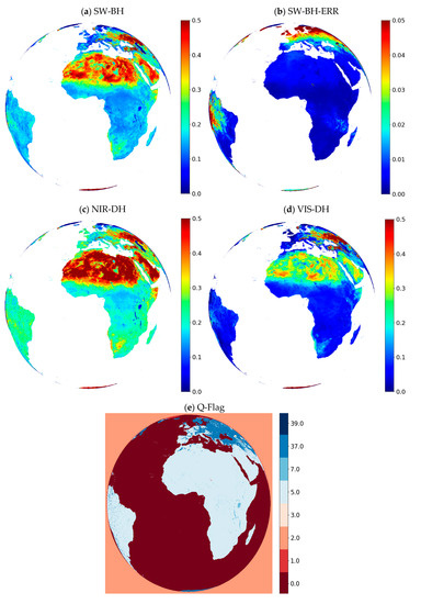
Figure 1.
Broadband MTAL-R albedo for January 15, 2012: (a) Total short-wave bi-hemispherical (SW-BH); (b) total short-wave bi-hemispherical error (SW-BH-ERR); (c) near infrared directional-hemispherical (NIR-DH); (d) visible directional-hemispherical (VIS-DH); and (e) quality flag.
3. Validation Data and Protocol
The strategy employed for validation of satellite-derived surface albedo usually relies on an inter-comparison between similar satellite products in order to perform a comparison at the continental scale [45]. However, it must be considered that satellites have generally different overpass times and therefore sense the surface of the planet under different atmospheric conditions. These differences may put in risk the fairness of the comparison. Another common strategy is to perform a comparison against ground-based measurements. The limitation here is that satellite and ground-based measurements may not be representative of the other because of their different footprint sizes.
3.1. Product Requirements
Details of the different MSG albedo products that are used in this work are described in Table 1.

Table 1.
Satellite Application Facility for Land Surface Analysis (LSA SAF) Meteosat Second Generation (MSG)-based MSG Ten-day Albedo (MTAL) surface albedo product characteristics.
Performance criteria such as mean bias error (MBE), relative mean bias error, and root mean square error (RMSE) have been considered and the obtained scores are compared against the accuracy requirements from Table 2. The requirement set by EUMETSAT is more relaxed than the GCOS accuracy requirement (5% accuracy), which appears today difficult to achieve for surface albedo derived from space-borne observations. The EUMETSAT requirement corresponds to the threshold requirement (10% accuracy) defined by World Meteorological Organization (WMO) for surface albedo. These requirements were decided within the LSA SAF, while taking into account the user needs and are given for the total shortwave bi-hemispherical broadband (SW-BH) albedo. Hence, this article only presents the results obtained from the validation of the SW-BH albedo product. The target accuracy for bias errors are given in relative units for albedo values larger than 0.15 and in absolute units for albedo values lower than 0.15.
Table 2.
LSA SAF MSG-based product requirements for MTAL SW-BH.
3.2. Validation Protocol
The strategy followed to assess the quality of the MTAL-R product is based on two different approaches.
On the one hand, in Section 4.1 a set of ground albedo stations are considered from various networks including Agoufou, Banizoumbou, Evora, Gobabeb, Niamey, Payerne, and Toravere. The data collected by these European and African stations are used to qualitative assess the MTAL-R product. For the sake of comparison, surface albedo data derived from the SPOT-VGT satellite are also included. The strategy to calculate comparable albedo values for MTAL-R and SPOT-VGT is discussed in Section 3.3.3.
On the other hand, the assessment of MTAL-R is extended spatially by using concomitant satellite albedo data from SPOT-VGT and MODIS. Here temporal and spatial analyses are performed to detect abnormal differences:
- First, Section 4.2 describes the temporal analysis that is done for a period of 10 years between 2004 and 2014. The analysis is performed over several ground reference sites from the AERONET network (https://aeronet.gsfc.nasa.gov/). Here, a large number of stations (337) were selected to get statistics representative of all the regions included in the MSG-disk (Europe, Africa and South America). MTAL-R is compared to SPOT-VGT and statistics are drawn up by considering regions of 50 km by 50 km centered on the AERONET stations. The strategy to estimate the mean albedo for each satellite product is given in Section 3.3.3.
- Second, Section 4.3 reports the spatial analysis that is performed over the SEVIRI grid. Surface albedo data (SW-BH) for the year 2012 is considered for this analysis. MTAL-R derived SW-BH albedo product is compared to SPOT-VGT and MODIS albedo products after a data re-projection to the SEVIRI grid.
In view of the product requirements (see Table 2) statistics are shown and discussed considering two albedo regimes: Lower than 0.15, and greater than 0.15. For the sake of simplicity, we will refer throughout the text to MTAL-R SW-BH product as MTAL-R. The three experiments are summarized in Table 3.
Table 3.
Validation protocol.
3.3. Surface Albedo Data Used for Comparison
3.3.1. Ground Observations
Seven ground stations from several networks are considered for the assessment of MTAL-R (Figure 2):
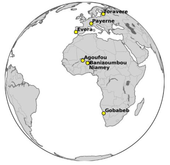
Figure 2.
Location of the ground measurement stations.
- Agoufou (Mali), Niamey (Niger), Banizoumbou (Niger)—AMMA (http://bd.amma-catch.org/amma-catch2/main.jsf)
- Gobabeb (Namibia), Evora (Portugal)—LSA SAF (http://lsa-saf.eumetsat.int/)
- Toravere (Estonia), Payerne (Switzerland)—BSRN (http://bsrn.awi.de/)
The mechanism to generate albedo data from ground measurements is as follows. Radiation data are acquired every 1 to 3 min. Measurements acquired with a solar zenith angle larger than 80° are discarded. The downward and upward measurements are divided to estimate the surface albedo at high temporal frequency. Finally, all the values obtained over a given day are averaged to produce a daily surface albedo value. This method differs from the approach proposed by [45] that calculates the total upward and downward shortwave radiations during the daytime in the first place to then make the ratio between the two daily variables (upward and downward). The importance of the averaging strategy should be carefully evaluated in further studies in order to define good practices and a common validation protocol (for SW-BH, SW-DH and maybe also SW blue-sky albedo).
3.3.2. Satellite Products
Satellite albedo products are generally provided for the DH and BH definitions. Albedo values are integrated over the three typical spectral domains, VIS, NIR and SW. As discussed earlier, the focus of this article is on the SW-BH albedo. Note that although MTAL-R and SPOT-VGT share the same SW spectral domain [0.3 to 4 µm], MODIS products considers a slightly wider spectral interval [0.3 to 5 µm]. Nonetheless, the comparison with MODIS products should still be significant as the solar energy between 4 and 5 microns is not significant compared to the rest of the solar spectral domain.
3.3.2.1. SPOT-VGT Surface Albedo Product
The Copernicus Global Land Service provides a land surface albedo product from SPOT-VGT satellite data. The retrieval method that is used for the version 1 of this product was designed in the framework of the FP5/CYCLOPES project [46]. This albedo product has a production period of around 10 days and a synthesis period of 30 days. The dates associated to the frequency of production depends on the age of the last observation used during the composite period. More details can be found in the product user manual for the surface albedo product from SPOT-VGT (http://land.copernicus.eu/global/products/sa; GIOGL1_PUM_SAV1, issue I1.10—last time consulted on 22 May 2018). The surface albedo products are delivered in 10 by 10 degrees tiles of around 1 km × 1 km resolution. The SPOT-VGT surface albedo product for the period between January 2004 and May 2014. All the data were used for our evaluation exercise. Only SW-BH surface albedo was considered for the validation procedure to agree with the MTAL-R product. We refer to this product as SPOT-VGT in the rest of the document.
3.3.2.2. MODIS Surface Albedo Product
MODIS land surface albedo data are widely used by the satellite and modeling community for evaluating other satellite albedo data and for refining the models. MODIS surface albedo MCD43B3 product is provided at 1 km of resolution and comes as a gridded product on a sinusoidal projection. The production period is of 8 days and the synthesis period of 16 days (https://lpdaac.usgs.gov/dataset_discovery/modis/modis_products_table/mcd43b3—last time consulted on 22 May 2018; [47]). The scientific team of MODIS combines both Terra and Aqua satellite observations. More information on the surface albedo retrieval algorithm implemented for MODIS is found here: https://modis.gsfc.nasa.gov/data/atbd/atbd_mod09.pdf. For the current exercise, we have used the collection 5 of MODIS combined product (MCD43B3) together with its quality flag (MCD43B2, https://lpdaac.usgs.gov/dataset_discovery/modis/modis_products_table/mcd43b2). We also consider the SW-BH product provided in MCD43B3 to agree with MTAL-R. Therefore, the SW-BH product from MCD43B3 is referred to as the MODIS albedo product in the rest of the document. Aspects concerning the preprocessing and the re-projection of MODIS combined data are discussed in Section 3.3.3. MODIS surface albedo products are considered only for the year 2012.
3.3.3. Preprocessing of Data for Validation
The intermediate steps that were needed to construct the various albedo products for comparison are explained here.
3.3.3.1. Data Selection Based on Quality Information
Ground truth—Data collected at ground stations undergo a filtering process prior to being released. Data that are contaminated or affected for any reason (e.g., sensor failure) are assigned to missing values. This information has been considered in our study, and the corresponding time slot is tagged as bad quality.
MODIS—Only those MODIS albedo pixels with corresponding good BRDF quality are kept for our study (i.e., BRDF Albedo Quality Flag = 0).
SPOT-VGT—Albedo data from SPOT-VGT are filtered out using the quality information within the NMOD flag. NMOD gives information about the valid number of observations used that were in the process of inversion. The albedo values are only considered in our study when the corresponding NMOD value is greater than two.
MTAL-R—For the case of MTAL-R, again only good quality data are considered. The error of covariance is considered in the filtering process with the rule: If is greater than 10% of the albedo value, the data are discarded.
3.3.3.2. Interpolation in Time
Ground truth—While MTAL-R is a 10-daily product, ground stations produce albedo data mostly on a daily basis. Therefore, for the computation of the statistics, only the ground truth data that are the closest in time with respect a corresponding MTAL-R date are considered (provided that both albedo values have passed the quality check on this date). The same procedure applies for satellite albedo data derived from SPOT-VGT.
Satellite products—The MTAL-R is processed at the 5th, 15th and 25th of each month. These dates are used as reference for inter-comparisons with other satellite products. The production of SPOT-VGT albedo data is very close to the production dates of MTAL-R (on the 3rd, 13th and 24th most of the times, see land.copernicus.vgt.vito.be/). Hence, for the purpose of validation the closest in time of SPOT-VGT albedo data are used to compare with MTAL-R. The same rule applies for MODIS with the difference that the closest date to MTAL-R is not always the same from month to month (as a result of the 8-day production period).
3.3.3.3. Strategy for Constructing Equivalent Spatial Albedo Values
MTAL-R versus ground truth, with indirect comparison with SPOT-VGT—For comparisons with ground observations, the MTAL-R albedo value of the pixel containing the ground station is selected. SPOT-VGT has a 1 km × 1 km pixel resolution whereas MTAL-R is at the resolution of the native SEVIRI grid (non-regular). Therefore, the SPOT-VGT pixels falling into the area defined by the MTAL-R pixel will be selected. If more than one pixel is selected for SPOT-VGT, the final SPOT-VGT albedo value is obtained after averaging the values of all the selected pixels.
MTAL-R versus SPOT-VGT: Temporal domain—Another strategy is applied for inter-comparisons between MTAL-R and SPOT-VGT on the temporal domain. For a given ground station, a 50 km by 50 km box is defined on the SPOT-VGT map, where the coordinates of the ground station approximately coincide in the center of the box. The limits of the box are used to select the equivalent region for the MTAL-R data. Valid albedo values observed from the selected MTAL-R and SPOT-VGT pixels are averaged to infer one MTAL-R and one SPOT-VGT measurement, respectively. This spatial upscaling to a resolution of 50 km by 50 km may lead to an artificial accuracy rising, as the different biases corresponding to all pixels in the box could compensate each other. However, the choice of not using the original MTAL-R pixel size was motivated by the non-regular size and shape of MSG/SEVIRI pixels. A unit in the SEVIRI grid looks like a diamond-shaped area (or a quadrilateral). And MSG grid size is around 3 km at the sub-satellite point over Africa, 5 km over Europe, and 20 km at the border of the disk.
MTAL-R versus other satellite products: Spatial domain—The inter-comparison in the spatial domain in Section 4.3 suggests another strategy. Because the different satellite products differ in their spatial resolution, it was decided to re-project both MODIS and SPOT-VGT to match the MSG pixel grid, which varies from the equator (3 km) to high latitudes (up to 20 km). Because both SPOT-VGT and MODIS albedo products are released in tiles with different projections, two different methods had to be employed prior to performing the spatial inter-comparison with MTAL-R:
- SPOT-VGT data are observed separately for the continental tiles of Europe, Africa, North-America, South-America and Asia. Because the MSG-disk comprises Europe, Africa, North-America, a big part of South-America and a small part of Asia, it was decided to only use the first three continental tiles. After merging them on a global map they were re-projected onto the MSG-SEVIRI grid. Only data from the year 2012 were considered for this exercise.
- MODIS products are released in the form of 10° longitude × 10° latitude tiles in a sinusoidal projection. In a first step, the tiles are aggregated with the help of the MODIS Reprojection Tool (MRT) to form a global data file that is later re-sampled onto an equirectangular projection. The resulting global data files in the new projection are re-projected again onto the MSG-SEVIRI grid. This approach is applied for MODIS data for the year 2012.
The spatial inter-comparison applies to a pixel-by-pixel analysis for the entire domain. For each pixel, at each date the bias between two products is calculated over the period of study (the year 2012 here). The spatial bias matrix values between satellite products are then appended to form a vector on temporal dimension. This vector is then averaged, and the mean value is displayed on the spatial map. Whenever a missing value occurs the corresponding date is not considered in the calculation of the mean. Density scatter plots of average albedo values over the year 2012 are also shown and results are discussed.
4. Results
4.1. MTAL-R versus Ground Truth, Indirect Comparison with SPOT-VGT
This section examines how MTAL-R compares to SPOT-VGT with respect to ground measurements for the ground stations listed in Section 3.3.1. This section does not aim to evaluate the quality of the MTAL-R product. In fact, the results of the comparison with ground measurements are only illustrative of the correlation that exists between both data, but must not be taken as a fair comparison due to the lack of spatial representativeness between the ground measurement and the SEVIRI acquisition. Results that are reported in Figure 3 are only indicative. Ground measurements are tagged either clear-sky or cloudy-sky.

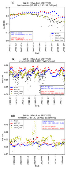
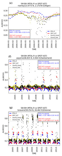
Figure 3.
Time series of MTAL-R against ground measurements for a set of ground stations: (a) Agoufou; (b) Banizoumbou; (c) Evora; (d) Gobabeb; (e) Niamey; (f) Payerne and (g) Toravere. SPOT-VGT derived equivalent albedo measurements are also presented. Difference statistics (root mean square error (RMSE), and mean bias error (MBE)) between satellite estimates and ground measurements are included. N is the number of satellite albedo estimates for which a ground measurement is available (and thus, the number of estimates used to calculate the statistics).
The plots in Figure 3 indicate that MTAL-R and SPOT-VGT have a similar behavior, as reflected by the RMSE and MBE scores. It should be noted here that different time periods are observed for MTAL-R and SPOT/VGT in view of the availability of the ground measurements. For example, only few months of data were available for Agoufou and Banizoumbou while as Toravere had more than 10 years of data. Discrepancies between satellite-based albedo and ground measurements are noticeable. These differences can be explained by the limited coverage of the ground-based observations (between 1 m to 10 m dependent on the tower height) compared to the satellite observations, which are representative of a wider spatial region (between 1 km to up to 20 km). In addition, local snow episodes lead to potentially high albedo values observed in the ground measurements that are usually not captured by the satellite products, leading to underestimations. These discrepancies, which were discussed in detail by [28,45], are often associated to the partial shade of the snow-covered ground by surface elements (e.g., trees, buildings). Upscaling from ground “point” measurements to the satellite spatial resolutions is a critical step and different methods are currently being developed to deal with this validation issue [48]. The coarse size of MSG/SEVIRI pixels (greater than 3 km) still needs extra efforts to envisage this spatial upscaling.
4.2. MTAL-R versus SPOT-VGT: Temporal Domain
MTAL-R is compared to its SPOT-VGT counterpart over time. This comparison is performed over 337 AERONET sites located in Europe, Africa, and South America.
In Section 4.2.1 time series of MTAL-R versus SPOT-VGT surface albedo measurements obtained following the strategy presented in Section 3.3.3 are displayed for a few cases. In Section 4.2.2, the mean surface albedo values are calculated for all sites, both for MTAL-R and SPOT-VGT, and the comparison over time is given. The density scatter plot that enables the global comparison of MTAL-R and SPOT-VGT is also given. Finally, in light of the requirements prescribed in Table 2 a pass/fail tag has been associated to all sites whenever available (see Section 4.2.3).
4.2.1. Time Series
Figure 4 displays time series of MTAL-R versus SPOT-VGT for a selection of AERONET reference sites. 16 stations were selected according to the diversity in their temporal dynamics. The following Section 4.2.2 shows the mean statistics over all the stations. The advantage of using the stations of the AERONET network for the evaluation of MTAL is that we dispose of well documented local land characteristics. This local information may provide a general overview of the surface characteristics at the pixel size (for example for Agoufou on https://aeronet.gsfc.nasa.gov/new_web/photo_db/Agoufou.html).
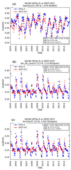

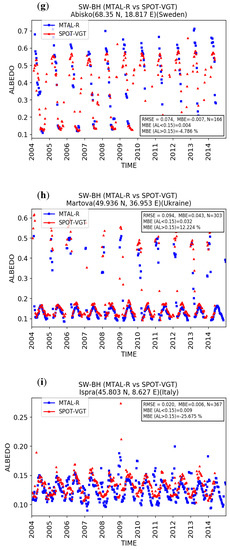

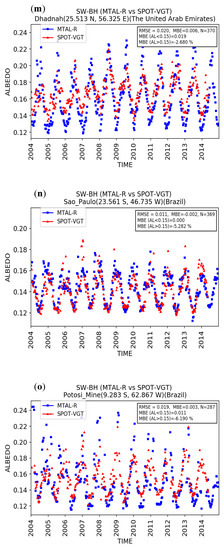
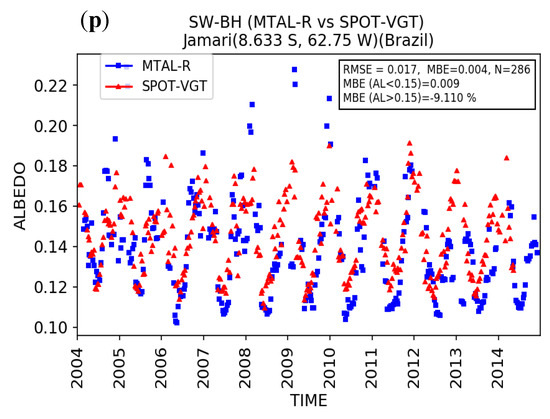
Figure 4.
Time series of MTAL-R versus SPOT-VGT for a selection of sites, viz: (a) Agoufou; (b) Ahi de Cara; (c) Armilla; (d) IASBS; (e) IER_Cinzana; (f) Saada; (g) Abisko; (h) Martova; (i) Ispra; (j) Baneasa; (k) Moldova; (l) Minsk; (m) Dhadnah; (n) Sao-Paulo; (o) Potosi_mine and (p) Jamari, for the period between 2004 and 2014.
Figure 4 shows that MTAL-R compares well to SPOT-VGT for the considered sites. Again, the seasonality is well captured. No break or abnormal trend is noticeable. However, low discrepancies exist potentially due to the differences of angular sampling between the sensors, which is crucial in the inversion of the BRDF.
4.2.2. Time Series of the Mean Bias for All Sites
In order to draw global conclusions Figure 5 displays the difference between MTAL-R and SPOT-VGT averaged over all 337 sites between 2004 and 2014. For the calculation of the mean bias, MTAL-R values below 0.15 are considered. For the calculation of the mean relative bias MTAL-R values greater than 0.15 are considered. These aspects derive from the definition of the requirements in Table 2.
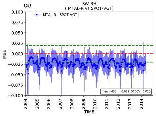
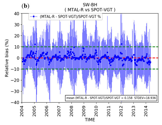
Figure 5.
Time series of the mean bias and mean relative bias of MTAL-R versus SPOT-VGT for all 337 AERONET reference sites located in Africa, Europe, and South America, when MTAL-R is (a) less than 0.15 and (b) greater than 0.15. The green dotted lines in the plot correspond to the product requirement values. The blue vertical lines represent the standard deviation for each date.
From Figure 5b, we see that MTAL-R meets the requirements (cf. Table 2) for the case when MTAL-R values are greater than 0.15. However, from Figure 5a, one sees that it does not meet the requirement for the other case when MTAL-R values lower than 0.15. Moreover, Figure 5a shows that for albedo values lower than 0.15 the statistical scores have a seasonal dependency with an overall underestimation of MTAL-R compared to SPOT-VGT. Low values (<0.15) of MTAL-R usually meet the requirements in the summer time and usually do not meet the requirements in the winter time due to the increase of the underestimation for this period of the year. Our MTAL albedo is based on SEVIRI data that correspond to up to 96 observations per day, thus providing a better description of the surface BRDF for high zenith angles. Consequently, the weight of cast shadows of trees, crops, and other surfaces becomes more important in MTAL-R compared to SPOT-VGT albedo (for which only one or two observations per day are used). The differences in the angular geometry sampling between MSG and SPOT-VGT can explain the underestimation of MTAL-R with respect to SPOT/VGT in winter. The differences of surface BRDF derived from observations from polar orbiting and geostationary platforms was discussed in References [28,49].
The albedo value pairs (on all 337 sites) between SPOT-VGT and MTAL-R are represented as a density scatter plot over the period of study (2004–2014) and is shown here as Figure 6. Overall, MTAL-R albedo values are lower than SPOT-VGT’s with an MBE of −0.012. For albedo values of MTAL-R less than 0.15, MTAL-R albedo values are smaller than SPOT-VGT with an MBE of −0.022. However, for MTAL-R albedo values greater than 0.15, MTAL-R albedo values are greater than SPOT-VGT with a relative mean bias error value of 0.158%. The results are consistent with those in Figure 5.

Figure 6.
Density scatter plot of MTAL-R versus SPOT-VGT for all 337 sites during the period 2004 and 2014. Statistical scores are also shown in the figure. For the calculation of the score one considers y-x or MTAL-R–SPOT-VGT.
4.2.3. Pass Rate for the MTAL-R Requirement Thresholds
The position of the AERONET reference sites that are considered for the comparison are shown in Figure 7. This figure also shows the pass/fail status for MTAL-R by means of the color coding. Figure 7a addresses the case where MTAL-R albedo values are less than 0.15 while Figure 7b addresses the case where MTAL-R values are greater than 0.15. Statistics are summarized in Table 4.

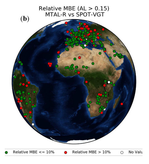
Figure 7.
Position of the AERONET reference sites used in the validation exercise of MTAL-R versus SPOT-VGT and their pass/fail status with respect to the requirements: (a) MTAL-R < 0.15; (b) MTAL-R > 0.15. Green is pass, and red is fail.
Table 4.
Pass/fail rate for all sites and for both cases of MTAL-R less than 0.15 and greater than 0.15.
Because some sites present only high (resp. low) albedo values greater (resp. lower) than 0.15 they do not contribute to the case MTAL-R < 0.15 (resp. MTAL-R > 0.15), these sites are not considered in the statistics shown in Table 3 and they appear with the tag “No Value” in Figure 7a (resp. Figure 7b). There are 67 such sites (respectively 14 sites) among the 337 stations. Figure 7a shows that most sites where MTAL-R data (for MTAL-R < 0.15) successfully pass the requirement are located in Brazil, Eastern Europe and southern Africa. For many of the selected European sites, MTAL-R data do not pass the requirement. The proportion of “pass” sites is a lot better for the case MTAL-R > 0.15 as observed from Table 4. In contrast to the previous case, the distribution of these sites is rather homogeneous as observed from Figure 7b.
Finally Figure 8 shows the pass rate per land cover type. This information on the type of surface is retrieved from the MODIS Land Cover product, which provides a global map with 17 land cover types. The MODIS Land Cover product at 5’ of resolution was used [50]. For our study, we assigned the predominant land cover type corresponding to the MODIS land cover type map from 2010 to each 50 km × 50 km box centered over the AERONET stations. In a second time, the pass rate results given in Figure 7 are split by cover type. Again, the results are given for the two regimes of albedo values. On the one hand, MTAL-R albedos lower than 0.15 show a pass rate higher than 50% for all cover types except for “Cropland/Natural vegetation mosaic”, “Urban and built-up”, “Croplands”, “Grasslands”, and “Water” (which corresponds to stations on small islands or along the coastlines). On the other hand, the pass rate for albedo values higher than 0.15 is higher than 50% for all cover types except for “Mixed Forest”.

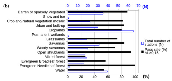
Figure 8.
Pass rate per land cover type from the MODIS Land Cover product. Results are given for the two regimes of albedo values: (a) Lower than 0.15; and (b) bigger than 0.15.
4.3. MTAL-R versus SPOT-VGT and MODIS: Spatial Domain
In this section the comparison between MTAL-R and other satellite products, namely SPOT-VGT and MODIS is performed over the spatial domain. Information on the preprocessing steps for all three products is detailed in Section 3.3.3. Figure 9 shows the spatial maps of the mean SW-BH bias, observed between various satellite products for the year 2012.

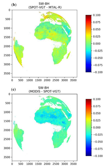
Figure 9.
Spatial maps of the mean bias observed the year 2012 between the satellite-based product pairs, (a) MODIS and MTAL-R; (b) SPOT-VGT and MTAL-R and (c) MODIS and SPOT-VGT.
It is clear from Figure 9 that MTAL-R is negatively biased over Europe, compared to MODIS and SPOT-VGT, whereas it is positively biased over Northern Africa and the Arabic peninsula.
Figure 10 represents the same data in the form of density scatter plots. If MODIS (SPOT-VGT) is considered as a valid reference, an MBE of −0.005 (−0.015) was observed for MTAL-R albedo values less than 0.15. A relative mean bias value of 6.173% (−1.511%) was observed for MTAL-R albedo values greater than 0.15. Consequently, MTAL-R meets the requirements of Table 2 in both cases.

Figure 10.
Density scatter plots for the inter-comparison of (a) MTAL-R versus MODIS; (b) MTAL-R versus SPOT-VGT and (c) SPOT-VGT versus MODIS during the period 2012.
5. Discussion and Summary
This study presented the new MTAL albedo product based on MSG data. The scientific algorithm was described in Section 2. The key feature of the MTAL algorithm is that surface components are represented by a kernel-driven BRDF model allowing fast and accurate computations of surface albedo. Moreover, MTAL averages over the 31-day composite window of BRDF properties retrieved on a daily basis. We believe that this approach may be more robust compared to temporal compositing done by other approaches (e.g., MODIS and SPOT-VGT). Indeed, a single mathematical inversion of the surface BRDF, using the entire set of observations collected for a composite period of several days, may lead to unrealistic BRDF parameters (i.e., negative or out of physical range). This could happen in case of rapid changes of the surface directional properties or when the temporal variations of two different kernel parameters are quite different (for example, a rapidly varying isotropic parameter with a stationary geometric parameter). On the contrary, the inversion on a daily basis that is done by MTAL attenuates this issue and has a better chance to be in accordance with the physical part of these semi-empirical BRDF models. A disadvantage of our approach is the semi-empirical (or semi-physical) construction of the kernel-based BRDF function. Although BRDF models are in constant improvement to better represent geometric, volumetric and other effects (such as hotspots), they have the inherent limitation of being partly empirical.
Compared to MTAL-R CDR product, NRT MTAL product is highly dependent on the availability of the auxiliary input fields and on any problem inherent to the product generation. For example, the architecture of the LSA-SAF processing chain required to be changed in 2012. Due to an important system failure occurred by that time, the LSA-SAF team decided in agreement with EUMETSAT to give a lower priority to the production of several products including MTAL. Consequently, MTAL NRT product was available only for 4 dates in 2012. This is a major argument to support the reanalysis activities presented in this manuscript. However, the statistics of difference between MTAL and MTAL-R products are very small (MBE = −0.0002 and RMSE = 0.018 for SW-BH over the 2011–2013 period). Furthermore, the accuracy of these two products (MTAL, MTAL-R) is deemed comparable.
For the validation of MTAL-R two accuracy indications are prescribed for two classes of albedo values (see Table 2). For MTAL-R values below 0.15 we expect an MBE less than 0.02 with respect to the reference data, while for MTAL-R values above 0.15, the relative bias error shall be less than 10%. The exercise of validation presented in Section 4 has compared MTAL-R albedo data with ground measurements as well as other satellite products, viz. MODIS and SPOT-VGT, both with similar spectral characteristics as MTAL-R. The comparison has been done on both the temporal and spatial dimensions. For the temporal comparison, we have used all the CDR of MTAL-R albedo data that are currently available (from 2004 to 2014). For the spatial comparison, only the year 2012 was considered.
A temporal inspection was performed by comparing MTAL-R and SPOT-VGT with ground measurements for seven stations in Europe and Africa. Direct validation of satellite-derived albedo with ground measurements is difficult due to the lack of spatial representativeness between the ground station footprint and the SEVIRI pixel. Despite discrepancies with the ground measurements, it is shown that MTAL-R captures well the seasonality of the surface albedo (compared to SPOT-VGT). These findings are mostly explained by the difference in size of the area of observation for ground-based or satellite-based measurements. This is further supported by the fact that MTAL-R compares well to SPOT-VGT at these stations.
BH albedo is often assumed to be comparable to ground observations of albedo acquired for cloudy conditions (when downward radiation is totally diffuse—see Figure 1 in Reference [28]). However, satellite measurements in the optical domain do not provide information on the surface properties under cloudy conditions. BH albedo is theoretically calculated as the angular integration of DH albedo (see Equation (6)). Furthermore, it is assumed to be more stationary in time than the DH counterpart, as it has no directional dependency. However, Figure 2 shows that ground measurements under cloudy conditions (black dots) can fluctuate significantly. For example, ground measurements under cloudy conditions in Niamey, Evora, and Banizoumbou suddenly decrease to very low values. This behavior may be the consequence of rainfall events, which rapidly darken soil surfaces. Another cause could be different atmospheric conditions that would impact the downward solar spectrum. Because surface albedo is defined as the ratio between the upward and downward solar flux at the Earth surface, for the broadband domain comprised between 0.3 µm and 4.0 µm (Equation (7)), spectral variations of the downward solar flux will infer changes on the measured broadband surface albedo even though the surface remains unchanged. Indeed, surface albedo is not necessarily an intrinsic property of the surface as already pointed out by Coakley in Reference [51] and especially in the presence of clouds. Hence, comparison between satellite BH albedo and ground measurements can become questionable, as well as the common understanding of BH albedo derived from satellite.
Another temporal inspection was taken over the period 2004 to 2014, by comparing MTAL-R with SPOT-VGT. The comparison was performed over boxes of 50 km × 50 km around a large number (337) of stations located in Europe, Africa and South America that are representative of a large variety of land cover types. Overall, MTAL-R albedo values tend to be lower than SPOT-VGT albedo values with an MBE of −0.012. This underestimation is observed for MTAL-R values below the 0.15 threshold, with an MBE of −0.022, while for MTAL-R above 0.15, MTAL-R albedo values are higher than SPOT-VGT with a relative mean bias error of +0.158%. If we consider SPOT-VGT as the valid reference, MTAL-R only meets the requirements for albedo values larger than 0.15 and does not meet the requirement for albedo values lower than 0.15. For albedo values lower than 0.15, we believe that the requirement may be too restrictive, as differences of angular sampling between polar orbiting and geostationary satellites may lead to surface BRDF discrepancies, especially in winter over mid and high latitudes (see Figure 5a and Figure 7a).
A spatial inspection was done by comparing MTAL-R with MODIS and SPOT-VGT. The analysis was performed for 2012 over the MSG/SEVIRI native grid. Polar orbiting satellite-based products (SPOT-VGT, MODIS) were re-projected over this grid in order to perform a pixel-by-pixel comparison. We found that over this test period, MTAL-R compares reasonably well against SPOT-VGT for the regions of Europe, Africa, and South America of the MSG-disk. Overall, MTAL-R albedo values are lower than SPOT-VGT with an MBE of −0.007. MTAL-R also compares well with MODIS, however MTAL-R albedo values are higher than MODIS with an MBE of 0.009. When looking separately at the two requirements, we see that for MTAL-R values below the 0.15 threshold (resp. above 0.15), MTAL-R albedo values are lower (resp. higher) than MODIS with an MBE (resp. relative MBE) of −0.005 (resp. +6.173%). In the comparison against SPOT-VGT, for MTAL-R values less than 0.15 (resp. greater than 0.15), MTAL-R albedo values are smaller than SPOT-VGT with an MBE (resp. relative MBE) of −0.015 (resp. −1.511%). If we consider MODIS or SPOT-VGT to hold as reference, MTAL-R meets the requirements of Table 2.
Several reasons could explain the differences of accuracy obtained between the spatial and the temporal analysis. In the spatial analysis over the MSG/SEVIRI grid, compensation effects between areas with positive and negative biases could induce a mean bias close to zero. Moreover, large forest areas (in boreal regions, in the Congo and in the Amazon) have very low albedo values all along the year. Very few of these dark forest areas were perhaps represented in the subset of 337 sites and we show that the MTAL algorithm shows limitations in the estimation of low albedo values for crops in winter. In any case, no temporal break or shift was observed in the albedo time series over the 337 stations for the 11-year period of the first CDR MTAL-R data set (2004–2014). This CDR data set will be completed with more years (2015 is now also available—last time consulted on 20 July 2018).
Overall, the comparison is satisfactory in order to qualify MTAL-R (LSA-150) albedo products with operational status, as it meets the requirements for almost all conditions, locations and periods of the year. Also, this validation study shows that this reprocessed CDR surface albedo product is mature enough to be used in modeling studies as well as for observing any potential trends. This work leads to 14 years of geostationary albedo products based on the second generation of European geostationary satellites. Today the continuity is ensured with the forthcoming Meteosat Third Generation (MTG) satellites to be launched in 2021. Consistent production of land surface albedo data is guaranteed until at least the end of the next decade thanks to EUMETSAT and its member states. Via the release of satellite products on ECVs, the LSA SAF provides a great opportunity to monitor and identify human-induced climate change, to analyze climate trend, and to monitor changes of vegetation properties. Finally, the geostationary LSA SAF products will also be used for the verification of the complementary long term polar albedo ECV products that will be developed in the framework of the Copernicus Climate Change Service (C3S) (https://climate.copernicus.eu/).
Author Contributions
D.C. conceived the product algorithm and designed the experiments. S.M., G.L. and D.C. performed the experiments. X.C., F.P., S.C.F. and I.F.T. analyzed the results. S.C.F. and I.F.T. provided technical support for implementation of the algorithms in LSA SAF operational chain. D.C., X.C., S.M., G.L. and I.F.T. wrote the article.
Funding
This research received no external funding.
Acknowledgments
The work presented in this article has been carried out as part of the validation activities of the SEVIRI land surface albedo dataset MTAL-R provided by the EUMETSAT Satellite Applications Facility on Land Surface Analysis (LSA-SAF; http://lsa-saf.eumetsat.int).
Conflicts of Interest
The authors declare no conflicts of interest.
References
- Intergovernmental Panel on Climate Change (IPCC). Climate Change 2014: Synthesis Report. Contribution of Working Groups I, II and III to the Fifth Assessment Report of the Intergovernmental Panel on Climate Change; Core Writing Team, Pachauri, R.K., Meyer, L.A., Eds.; IPCC: Geneva, Switzerland, 2014; p. 151. [Google Scholar]
- Lattanzio, A.; Schulz, J.; Matthews, J.; Okuyama, A.; Theodore, B.; Bates, J.J.; Knapp, K.R.; Kosaka, Y.; Schüller, L. Land Surface Albedo from Geostationary Satelites: A Multiagency Collaboration within SCOPE-CM. Bull. Am. Meteorol. Soc. 2013, 94, 205–214. [Google Scholar] [CrossRef]
- He, T.; Liang, S.; Yu, Y.; Wang, D.; Gao, F.; Liu, Q. Greenland surface albedo changes in July 1981–2012 from satellite observations. Environ. Res. Lett. 2013, 8, 044043. [Google Scholar] [CrossRef]
- Bazile, E.; El Haiti, M.; Bogatchev, A.; Spiridonov, V. Improvement of the snow parameterization in ARPEGE/ALADIN. In Proceedings of the SRNWP/HIRLAM Workshop Surface Processes, Turbulence and Mountain Effects, Madrid, Spain, 22–24 October 2001. [Google Scholar]
- Crook, J.A.; Forster, P.M. Comparison of surface albedo feedback in climate models and observations. Geophys. Res. Lett. 2014, 41, 1717–1723. [Google Scholar] [CrossRef]
- Global Climate Observing System (GCOS). Implementation Plan for the Global Observing System for Climate in Support of the UNFCCC; Report GCOS-92 (WMO/TD No. 1219); GCOS: Asheville, NC, USA; 2004; 136p. [Google Scholar]
- Munier, S.; Carrer, D.; Planque, C.; Camacho, F.; Albergel, C.; Calvet, J.-C. Satellite Leaf Area Index: Global scale analysis of the tendencies per vegetation type over the last 17 years. Remote Sens. 2018, 10, 424. [Google Scholar] [CrossRef]
- Grenfell, T.C.; Perovich, D.K. Seasonal and spatial evolution of albedo in a snow ice land ocean environment. J. Geophys. Res. 2004, 109, C01001. [Google Scholar] [CrossRef]
- Planque, C.; Carrer, D.; Roujean, J.-L. Analysis of MODIS albedo changes over steady woody covers in France during the period of 2001–2013. Remote Sens. Environ. 2017, 191, 13–29. [Google Scholar] [CrossRef]
- Lebourgeois, F.; Pierrat, J.-C.; Perez, V.; Piedallu, C.; Cecchini, S.; Ulrich, E. Simulating phenological shifts in French temperate forests under two climatic change scenarios and four driving global circulation models. Int. J. Biometeorol. 2010, 54, 563–581. [Google Scholar] [CrossRef] [PubMed]
- Csiszar, I.; Gutman, G. Mapping global land surface albedo from NOAA AVHRR. J. Geophys. Res. 1999, 104, 6215–6228. [Google Scholar] [CrossRef]
- Strugnell, N.C.; Lucht, W. An Algorithm to Infer Continental-Scale Albedo from AVHRR Data, Land Cover Class, and Field Observations of Typical BRDFs. J. Clim. 2001, 14, 1360–1376. [Google Scholar] [CrossRef]
- Leroy, M.; Deuzé, J.L.; Bréon, F.M.; Hautecoeur, O.; Herman, M.; Buriez, J.C.; Tanré, D.; Bouffiès, S.; Chazette, P.; Roujean, J.-L. Retrieval of atmospheric properties and surface bidirectional reflectances over the land from POLDER/ADEOS. J. Geophys. Res. 1997, 102, 17023–17037. [Google Scholar] [CrossRef]
- Wang, Z.; Schaaf, C.B.; Chopping, M.J.; Strahler, A.H.; Wang, J.; Roman, M.O.; Rocha, A.V.; Woodcock, C.E.; Shuai, Y. Evaluation of Moderate-resolution Imaging Spectroradiometer (MODIS) snow albedo product (MCD43A) over tundra. Remote Sens. Environ. 2012, 117, 264–280. [Google Scholar] [CrossRef]
- Schaaf, C.B.; Gao, F.; Strahler, A.H.; Lucht, W.; Li, X.; Tsang, T.; Strugnell, N.C.; Zhang, X.; Jin, Y.; Muller, J.-P.; et al. First Operational BRDF, Albedo and Nadir Reflectance Products from MODIS. Remote Sens. Environ. 2002, 83, 135–148. [Google Scholar] [CrossRef]
- Ba, M.B.; Nicholson, S.E.; Frouin, R. Satellite-Derived Surface Radiation Budget over the African Continent. Part II: Climatologies of the Various Components. J. Clim. 2001, 14, 60–76. [Google Scholar] [CrossRef]
- He, T.; Liang, S.L.; Wang, D.; Shi, Q.; Tao, X. Estimation of high-resolution land surface shortwave albedo from AVIRIS data. IEEE J. Sel. Top. Appl. Earth Obs. Remote Sens. 2014, 7, 4919–4928. [Google Scholar] [CrossRef]
- Franchistéguy, L.; Geiger, B.; Roujean, J.-L.; Samain, O. Retrieval of land surface albedo over France using SPOT4/VEGETATION data. In Proceedings of the 2nd International VEGETATION User Conference, Antwerp, Belgium, 24–26 March 2004; EUR 21552 EN. Antwerp, F., Veroustraete, E., Bartholomé, W., Verstraeten, W., Eds.; Office for Official Publications of the European Communities: Luxembourg, 2005; pp. 57–62. [Google Scholar]
- Carrer, D.; Smets, B.; Ceamanos, X.; Roujean, J.-L.; Lacaze, R. Copernicus Global Land SPOT/VEGETATION and PROBA-V Surface Albedo Products—1 Km Version 1; Algorithm Theoretical Basis Document, Issue 2.11, Copernicus Global Land Operations Vegetation and Energy CGLOPS-1, Framework Service Contract N° 199494; Japan Radio Company (JRC): Tokyo, Japan, 2018. [Google Scholar]
- Wang, D.; Liang, S.; He, T.; Yu, Y. Direct estimation of land surface albedo from VIIRS data: Algorithm improvement and preliminary validation. J. Geophys. Res. Atmos. 2013, 118, 12577–12586. [Google Scholar] [CrossRef]
- He, T.; Liang, S.; Wu, H.; Wang, D. Prototyping GOES-R albedo algorithm based on modis data. In Proceedings of the 2011 IEEE International Geoscience and Remote Sensing Symposium, Vancouver, BC, Canada, 24–29 July 2011; pp. 4261–4264. [Google Scholar]
- Geiger, B.; Carrer, D.; Franchisteguy, L.; Roujean, J.-L.; Meurey, C. Land surface albedo derived on a daily basis from Meteosat second generation observations. IEEE Trans. Geosci. Remote Sens. 2008, 46, 3841–3856. [Google Scholar] [CrossRef]
- Muller, J.P.; López, G.; Watson, G.; Shane, N.; Kennedy, T.; Yuen, P.; Lewis, P.; Fischer, J.; Guanter, L.; Domench, C.; et al. The ESA GlobAlbedo project for mapping the Earth’s land surface albedo for 15 years from European sensors. In Proceedings of the IEEE Geoscience and Remote Sensing Symposium (IGARSS), Munich, Germany, 22–27 July 2012. [Google Scholar]
- Muller, J.-P. GlobAlbedo Final Validation ReportRep.; University College London: London, UK, 2013; Available online: http://www.globalbedo.org/docs/ GlobAlbedo_FVR_V1_2_web.pdf (accessed on 31 July 2018).
- Liang, S.; Zhao, X.; Liu, S.; Yuan, W.; Cheng, X.; Xiao, Z.; Zhang, X.; Liu, Q.; Cheng, J.; Tang, H.; et al. A long-term Global LAnd Surface Satellite (GLASS) data-set for environmental studies. Int. J. Digit. Earth 2013, 6, 5–33. [Google Scholar] [CrossRef]
- Ceamanos, X.; Carrer, D.; Roujean, J.-L. Improved retrieval of direct and diffuse downwelling surface shortwave flux in cloudless atmosphere using dynamic estimates of aerosol content and type: Application to the LSA-SAF project. Atmos. Chem. Phys. 2014, 14, 8209–8232. [Google Scholar] [CrossRef]
- Drame, M.S.; Ceamanos, X.; Roujean, J.L.; Boone, A.; Lafore, J.P.; Carrer, D.; Geoffroy, O. On the Importance of Aerosol Composition for Estimating Incoming Solar Radiation: Focus on the Western African Stations of Dakar and Niamey during the Dry Season. Atmosphere 2015, 6, 1608–1632. [Google Scholar] [CrossRef]
- Carrer, D.; Roujean, J.L.; Meurey, C. Comparing operational MSG/SEVIRI land surface albedo products from Land SAF with ground measurements and MODIS. IEEE Trans. Geosci. Remote Sens. 2010, 48, 1714–1728. [Google Scholar] [CrossRef]
- Ohring, G.; Wielicki, B.; Spencer, R.; Emery, B.; Datla, R. Satellite Instrument Calibration for Measuring Global Climate Change: Report of a Workshop. Bull. Am. Meteorol. Soc. 2005, 86, 1303–1314. [Google Scholar] [CrossRef]
- Trigo, I.F.; Dacamara, C.C.; Viterbo, P.; Roujean, J.-L.; Olesen, F.; Barroso, C.; Camacho-de-Coca, F.; Carrer, D.; Freitas, S.C.; García-Haro, J.; et al. The Satellite Application Facility for Land Surface Analysis. Int. J. Remote Sens. 2011, 32, 2725–2744. [Google Scholar] [CrossRef]
- Carrer, D.; Pique, G.; Ferlicoq, M.; Ceamanos, X.; Ceschia, E. What is the potential of cropland albedo management in the fight against global warming? A case study based on the use of cover crops. Environ. Res. Lett. 2018, 13, 044030. [Google Scholar] [CrossRef]
- Lattanzio, A.; Fell, F.; Bennartz, R.; Trigo, I.F.; Schultz, J. Quality assessment and improvement of the EUMETSAT Meteosat Surface Albedo Climate Data Record. Atmos. Meas. Tech. 2015, 8, 4561–4571. [Google Scholar] [CrossRef]
- Bates, J.J.; Privette, J.L.; Kearns, E.J.; Glance, W.; Zhao, X. Sustained Production of Multidecadal Climate Records: Lessons from the NOAA Climate Data Record Program. Bull. Am. Meteorol. Soc. 2016, 97, 1573–1581. [Google Scholar] [CrossRef]
- Yang, W.; John, V.; Zhao, X.; Lu, H.; Knapp, K. Satellite Climate Data Records: Development, Applications, and Societal Benefits. Remote Sens 2016, 8, 331. [Google Scholar] [CrossRef]
- Loew, A. Terrestrial satellite records for climate studies: How long is long enough? A test case for the Sahel. Theor. Appl. Climatol. 2014, 115, 427–440. [Google Scholar] [CrossRef]
- Nicodemus, F.; Richmond, J.C.; Hsia, J.J.; Ginsberg, I.W.; Limperis, T. Geometrical Considerations and Nomenclature for Reflectance; NBS Monograph 160; U.S. Department of Commerce: Washington, DC, USA, 1977.
- Pinty, B.; Roveda, F.; Verstraete, M.M.; Gobron, N.; Govaerts, Y.; Martonchik, J.V.; Diner, D.J.; Kahn, R.A. Surface albedo retrieval from Meteosat. J. Geophys. Res. 2000, 105, 18099–18134. [Google Scholar] [CrossRef]
- Rahman, H.; Dedieu, G. SMAC: A simplified method for the atmospheric correction of satellite measurements in the solar spectrum. Int. J. Remote Sens. 1994, 15, 123–143. [Google Scholar] [CrossRef]
- Berthelot, B. Coefficients SMAC Pour MSG; Noveltis Internal Report NOV-3066-NT-834; Noveltis Internal: Ramonville Saint Agne, France, 2001. [Google Scholar]
- Derrien, M.; Le Gléau, H. MSG/SEVIRI cloud mask and type from SAFNWC. Int. J. Remote Sens. 2005, 26, 4707–4732. [Google Scholar] [CrossRef]
- Ceamanos, X.; Douté, S.; Fernando, J.; Schmidt, F.; Pinet, P.; Lyapustin, A. Surface reflectance of Mars observed by CRISM/MRO: 1. Multi-angle Approach for Retrieval of Surface Reflectance from CRISM observations (MARS ReCO). J. Geophys. Res. Planets 2013, 118, 540–559. [Google Scholar] [CrossRef]
- Press, W.H.; Teukolsky, S.A.; Vetterling, W.T.; Flannery, B.P. Numerical Recipes in Fortran; Cambridge University Press: Cambridge, UK, 1992. [Google Scholar]
- Roujean, J.-L.; Leroy, M.; Deschamps, P.-Y. A bidirectional reflectance model of the Earth’s surface for the correction of remote sensing data. J. Geophys. Res. 1992, 97, 20455–20468. [Google Scholar] [CrossRef]
- Lucht, W.; Lewis, P. Theoretical noise sensitivity of BRDF and albedo retrieval from the EOS-MODIS and MISR sensors with respect to angular sampling. Int. J. Remote Sens. 2000, 21, 81–98. [Google Scholar] [CrossRef]
- Wang, D.; Liang, S.; He, T.; Yu, Y.; Schaaf, C.; Wang, Z. Estimating daily mean land surface albedo from MODIS data. J. Geophys. Res. Atmos. 2015, 120, 4825–4841. [Google Scholar] [CrossRef]
- Geiger, B.; Samain, O. Albedo Determination, Algorithm Theoretical Basis Document of the Cyclopes Project; Version 2.0; Météo-France/CNRM: Paris, France, 2004. [Google Scholar]
- Strahler, A.H.; Muller, J.P.; MODIS Science Team Members. MODIS BRDF/Albedo Product: Algorithm Theoretical Basis Document, Version 5.0. USA. 1999. Available online: http://eunchul.com/Algorithms/BRDF/3.MODIS_BRDF_Albedo_Product_Algorithm_Theoretical_Basis_Do.pdf (accessed on 31 July 2018).
- Wu, X.; Xiao, Q.; Wen, J.; Liu, Q.; You, D.; Dou, B.; Tang, Y. Upscaling in situ albedo for validation of coarse scale albedo product over heterogeneous surfaces. Int. J. Digit. Earth 2017, 10, 604–622. [Google Scholar] [CrossRef]
- Matsuoka, M.; Takagi, M.; Akatsuka, S.; Honda, R.; Nonomura, A.; Moriya, H.; Yoshioka, H. Bidirectional reflectance modeling of the geostationary sensor HIMAWARI-8/AHI using a kernel-driven BRDF model. SPRS Ann. Photogramm. Remote Sens. Spat. Inf. Sci. 2016, 3, 3–9. [Google Scholar]
- Channan, S.; Collins, K.; Emanuel, W.R. Global Mosaics of the Standard MODIS Land Cover Type Data; University of Maryland and the Pacific Northwest National Laboratory: College Park, MD, USA, 2014. [Google Scholar]
- Coakley, J.-A. Reflectance and Albedo, Surface, Encyclopedia of the Atmosphere; Academic Press: Cambridge, MA, USA, 2003; pp. 1914–1923. [Google Scholar]
© 2018 by the authors. Licensee MDPI, Basel, Switzerland. This article is an open access article distributed under the terms and conditions of the Creative Commons Attribution (CC BY) license (http://creativecommons.org/licenses/by/4.0/).