Synergistic Effect of Multi-Sensor Data on the Detection of Margalefidinium polykrikoides in the South Sea of Korea


1
Korea Ocean Satellite Center, Korea Institute of Ocean Science and Technology (KIOST), 385 Haeyang-ro, Yeongdo-gu, Busan 49111, Korea
2
Ocean Science and Technology School, KIOST-Korea Maritime and Ocean University (KMOU), 727 Taejong-ro, Yeongdo-gu, Busan 49112, Korea
3
Jeju Marine Research Section, Korea Institute of Ocean Science and Technology (KIOST), 2670 Gujwa-eup, Jeju-shi 63349, Korea
*
Author to whom correspondence should be addressed.
Remote Sens. 2019, 11(1), 36; https://doi.org/10.3390/rs11010036
Submission received: 31 October 2018
/
Revised: 11 December 2018
/
Accepted: 21 December 2018
/
Published: 26 December 2018
(This article belongs to the Special Issue Selected Papers from the “International Symposium on Remote Sensing 2018”)
Abstract
:Since 1995, Margalefidinium polykrikoides blooms have occurred frequently in the waters around the Korean peninsula. In the South Sea of Korea (SSK), large-scale M. polykrikoides blooms form offshore and are often transported to the coast, where they gradually accumulate. The objective of this study was to investigate the synergistic effect of multi-sensor data for identifying M. polykrikoides blooms in the SSK from July 2018 to August 2018. We found that the Spectral Shape values calculated from in situ spectra and M. polykrikoides cell abundances in the SSK were highly correlated. Comparing red tide spectra from near-coincident multi-sensor data, remote-sensing reflectance (Rrs) spectra were similar to the spectra of in situ measurements from blue to green wavelengths. Rrs true-color composite images and Spectral Shape images of each sensor showed a clear pattern of M. polykrikoides patches, although there were some limitations for detecting red tide patches in coastal areas. We confirmed the complementarity of red tide data extracted from each sensor using an integrated red tide map. Statistical assessment showed that the sensitivity of red tide detection increased when multi-sensor data were used rather than single-sensor data. These results provide useful information for the application of multi-sensor for red tide detection.
1. Introduction
Harmful algal blooms (HABs), wherein accumulation of plankton causes discoloration of water, are increasing worldwide. They often cause high mortality of fish and shellfish, and by extension great economic losses in the aquaculture and tourism industries [1,2]. HABs in coastal regions cause major damage to aquaculture farms and have harmful effects on human health [3,4]. In Korean waters, Margalefidinium (previous called as Cochlodinium) polykrikoides [5] blooms have gradually become larger, wider, and more frequent since 1995. This species first bloomed in the South Sea of Korea (SSK) and has expanded to the West Sea (Yellow Sea) and East Sea (Sea of Japan) [6]. In the SSK, large-scale M. polykrikoides blooms that form offshore are often transported to coastal waters and gradually accumulate there [7]. This movement is caused by physical factors such as tidal currents, typhoons, wind, and the biological characteristics of red tide species. Thus, accurate and timely surveillance of M. polykrikoides blooms in the SSK, including both coastal and offshore waters, is needed to minimize the damage caused by such blooms. It is also necessary to establish an early warning system for M. polykrikoides blooms.
Red tide monitoring in Korean coastal waters has been conducted by the National Institute of Fisheries Science (NIFS) since 1972. Such monitoring has been carried out regularly at monitoring stations by national institutes such as NIFS, local governments, and the national maritime police agency since 1996 [6]. NIFS provides all types of available data, including biological, hydrological, meteorological, and remote sensing data, in published daily red tide reports [8]. Daily red tide reports include the causative organisms, cell abundance, and affected and warning areas. These reports also include predictions for the development and spread of on-going red tides. NIFS has adopted a red tide warning system for fishermen and aquaculturists consisting of three levels: red tide emergence attention, red tide attention, and red tide alert. The new red tide emergence attention notice was introduced in 2015, and is issued when the cell density of M. polykrikoides exceeds 10 cells mL−1. In addition, attention and alert notices are issued when the cell density exceeds 100 and 1000 cells mL−1, respectively [9]. However, because this information is obtained mainly through field sampling at discrete locations using in situ observations, the red tide areas across broader geographic scales are becoming more difficult to manage. In addition, there are limitations to monitoring in terms of manpower, cost, and time [10]. For this reason, limited information is available on the presence or absence of red tide patches and the spatial distribution of cell concentrations. M. polykrikoides blooms occur not only in nearshore areas, but also in offshore waters Thus, it is necessary to monitor all waters of the SSK. Remote sensing data are capable of wide area detection and thus may be effectively applied for quick and accurate monitoring when a red tide occurs.
Satellite-based algorithms have been developed for identifying and monitoring HABs [10,11,12,13]. Red tide detection from satellite data began with the use of chlorophyll concentration (CHL) data gathered by several ocean color sensors, including the Sea-viewing Wide Field-of-view Sensor (SeaWiFS) and MODerate resolution Imaging Spectroradiometer (MODIS) [3,14,15]. However, this method has several limitations, such as uncertainties in atmospheric correction, interference from various colored compounds, and the presence of other types of phytoplankton. When CHL of non-red tide species is very similar to that of red tide species, it is difficult to distinguish the red tide species. In addition, some red tide species have weak chlorophyll signals. Moreover, seawater signal in coastal areas is complex due to various constituents such as suspended particulate matter (SPM) and colored dissolved organic matter (CDOM) that cause the scattering and absorption. These spectral characteristics cause large overestimation of CHL in the SSK [16,17]. The fluorescence line height (nFLH) data and enhanced Red-Green-Blue (ERGB) images derived from MODIS or Medium Resolution Imaging Spectrometer (MERIS) have been used in place of CHL data for red tide detection [18,19,20]. However, distinguishing between red tide species and non-red tide species with similar CHL remains difficult. In particular, estimates of CHL may be inaccurate due to interactions between chlorophyll and the abundant SPM present in the SSK.
To overcome the limitation of red tide detection using CHL data, the optical properties of seawater have been used to detect red tides [12,13,21,22,23,24,25]. Dierssen et al. [21] and Sasaki et al. [22] found that the peak of remote-sensing reflectance (Rrs) in visible regions was shifted to long wavelengths (570–590 nm) region during red tide blooms. Cannizzaro et al. [23] reported that K. brevis blooms exhibit high CHL but low backscattering values. Wynne et al. [24] and Tomlinson et al. [12] suggested that the low backscattering observed in K. brevis blooms and low detrital absorption may affect the spectral reflectance curve in the blue portion of the visible region. Lou and Hu [25] developed a modified red tide index (MRI) based on the spectral characteristics of Prorocentrum donghaiense, which is low in the blue region but high in the green region. Other methods include the use of SPM and sea-surface temperature data collected during red tide blooms [11,26] and schematic processes of red tide and non-red tides through spectral classification techniques [16,27,28].
Most methods for red tide detection have been developed based on SeaWiFS, MODIS, and Geostationary Ocean Color Imager (GOCI), because ocean color sensors have higher spectral resolution and signal-to-noise ratio (SNR) than terrestrial sensors such as Landsat Enhanced Thematic Mapper Plus (ETM+), Operational Land Imager (OLI), and Sentinel-2 MultiSpectral Instrument (MSI). These characteristics lead to a high detection rate for red tide patches mixed with seawater and provide an excellent estimate of red tide abundance. Despite the many advantages of ocean color sensors, red tide information often cannot be acquired in coastal areas due to low spatial resolution and coastal masking caused by the uncertainty of atmospheric correction in coastal areas where turbidity is high. As an alternative to ocean color sensors, the use of terrestrial sensors is recommended. Compared with ocean color sensors, the spectral resolution of terrestrial sensors is low. On the other hand, they have excellent spatial resolution. Therefore, terrestrial sensors can provide useful information for red tide detection in coastal areas. In addition, because the terrestrial sensor has a band in the wavelength range used in the red tide detection algorithm, it can be employed with the existing algorithms.
A comprehensive approach based on the characteristics of each sensor is useful for accurate red tide detection over a wide range of conditions, including coastal and offshore areas. There are several issues caused by using multi-sensor data in red tide detection. Various factors such as spatial resolution, spectral resolution, SNR, the modulation transfer function (MTF), the difference in image acquisition time, atmospheric correction, and geo-referencing errors can affect the results of red tide detection. Due to these differences, even when the same red tide detection algorithm is applied to each sensor, the red tide distribution extracted may differ among the sensors. Because it is very difficult to consider all characteristics of various sensors, a red tide detection technique using multi-sensors requires further research. To date, few studies have employed multi-sensors for red tide detection. According to Wang et al. [29], the spatial resolution of HJ-CCD is better than that of MODIS. Thus, its extraction result is better than that of MODIS. Oh et al. [30] qualitatively compared red tide areas extracted from MODIS and GOCI. Tao et al. [13] noted that when an MRI [25] is applied to MODIS imagery (802 at 488 nm), high values are obtained for near-shore areas due to their low SNR compared to GOCI (1316 at 490 nm) in the blue band. Shin et al. [31] performed the red tide detection through image fusion of GOCI and Landsat OLI. Red tide detection in the coastal area is carried out using Landsat OLI, while GOCI was used in offshore waters with severe noise caused by sea current and ship trajectories. Using multi-sensor detection rather than a single-sensor, it is possible to extract red tide areas that are more similar to the true value due to improved accuracy of red tide detection.
The objective of this study was to identify a possible synergistic effect of multi-sensor data on the detection of M. polykrikoides blooms. For this purpose, we (1) investigated the specifications of various sensors to determine the pros and cons of each sensor’s data; (2) analyzed the spectral characteristics of waters containing M. polykrikoides obtained from in situ measurement; (3) compared Rrs true-color composite and Spectral Shape images created using multi-sensor data for visual inspection and comparison of red tide patches; (4) generated an integrated red tide map using all possible images; and (5) presented the results of statistical evaluation to identify the synergistic effect of multi-sensor data.
2. Materials and Methods
2.1. Study Area
The study area covers the SSK including Goheung, Yeosu, Namhae, and Tongyeong, which is bordered by a complex rias coastline structure (Figure 1). Three study areas were used. The dates of image acquisition were 29 July 2018, 30 July 2018, and 1 August 2018. The SSK contains many large and small islands. Most red tide patches that occurred near the coast were difficult to detect. The characteristics of seawater were very different between the coastal and offshore areas. Offshore waters has clear characteristic (Case-1 waters) due to the Kuroshio Current, but exhibits complex water characteristic in that the contents of SPM and CDOM increase toward coastal areas [16]. The depth range was 8–25 m in coastal areas and 27–54 m in offshore areas [7]. M. polykrikoides blooms occurred quite frequently in the study area. On July 24, 2018, attention notices were issued from Goheung to Namhae [8]. This notice was extended to Geoje on July 31 and ended on August 19, representing a small-scale bloom compared to previous years. The maximum abundance of M. polykrikoides was 4500 cells mL−1 at Bodolbada, located between Goheung and Yeosu.
2.2. In Situ Measurements
In situ observations of M. polykrikoides bloom were conducted on August 7 and August 8, 2018 in the coastal area in Yeosu and Namhae (Figure 1). Water samples were collected at 14 sampling locations in Yeosu and Namhae for measurement of CHL, the spectrum of surface waters, and cell abundance. Then, 25-mm Whatman GF/F glass fiber filters were used to collect samples under low vacuum pressure for CHL estimation. Samples were stored frozen in liquid nitrogen until laboratory analysis. Pigments were extracted from filters with 90% acetone and refrigerated at 4 °C for 24 h. CHL was estimated using the trichromatic equations reported by Jeffrey and Humphrey [32] after measuring pigment absorbance with a Perkin-Elmer Lambda 19 UV/VIS/NIR dual-beam spectrophotometer.
The spectra of surface water were measured at the sampling sites using a hyperspectral free-falling optical profiler (Profiler II; Satlantic Inc.) with a spectral range of 349–808 nm and a spectroradiometer (FieldSpec3; Analytical Spectral Devices) with a spectral range of 350–2500 nm. In three sampling locations (st. R02, Y01, and Y02), up-welling radiance, as well as up-welling and down-welling irradiance in water column were measured using Profiler II. Three measurements were performed at 1 m intervals considering the depth of each sample location. It was converted to mean value and measured values at sea surface were used in this study. Data processing was performed using ProSoft Software (Satlantic Inc.; Canada) with default constants, and finally Rrs is calculated. The spectra were measured using ASD at all sampling locations except for three sampling locations above. Total water-leaving radiance, sky radiance, and down-welling irradiance were measured by Spectroradiometer. All spectra were measured three times and averaged. Sky radiance caused by the air-sea interface was obtained by multiplying sky radiance by a constant of 0.025. Water-leaving radiance is the result of subtracting sky radiance from total water-leaving radiance. Finally, Rrs was calculated by dividing water-leaving radiance by down-welling irradiance.
Phytoplankton abundance was analyzed through droplet digital PCR (ddPCR), an advanced method to quantify the absolute copy number per M. polykrikoides cell [33]. This tool is known to improve the accuracy and sensitivity of monitoring M. polykrikoides abundance. Seawater collected from the various locations was filtered through cellulose acetate (CA) filters under relatively low vacuum and then subjected to DNA extraction. Then, the copy number of M. polykrikoides in seawater was analyzed using a species-specific marker (ITS primer) for M. polykrikoides. The cell abundance was estimated by conversion using the copy number per M. polykrikoides cell.
2.3. Image Processing
To determine the synergistic effect of multi-sensor data, ocean color and terrestrial sensor data were processed. Ocean color sensors included GOCI, as well as Sentinel-3 Ocean and Land Colour Instrument (OLCI). GOCI level 1B data were obtained from the Korea Ocean Satellite Center (KOSC) [34]. We converted level 1B data to level 2 using GOCI data processing software (GDPS, version 2.0) with the default parameters and standard atmospheric correction [35] and Rrs was used in this study. GOCI images were obtained at eight time points per day at hourly intervals from 00:15 GMT to 07:45 GMT. In this study, GOCI images acquired at 01:00 GMT were used. It is a geostationary satellite with an observation area covering Korea, Japan, the eastern coast of China, and parts of the northern coast of Taiwan. OLCI sensor onboard Sentinel-3 is a continuation of the ENVISAT MERIS sensor [36]. OLCI level-2 water full resolution (WFR) product was downloaded from the Copernicus Online Data Access Hub provided by the European Organisation for Meteorological Satellites (EUMETSAT) [37]. Oa* reflectance (Rrs) was coordinate-transformed using the Sentinel Application Platform (SNAP, version 6.0) developed by ESA. OLCI images of the area around the Korean peninsula were obtained at about 01:00 GMT every one to three days.
Landsat ETM+ and OLI images were downloaded from the U. S. Geological Survey [38]. The revisit periods of both sensors are 16 days. Data from the same region can be acquired every eight days. Landsat OLI has an increased bit depth of 12 compared to the Landsat Thematic Mapper (TM) and ETM+, which has 8-bit data [39]. The Sentinel-2 mission provides continuity for services relying on global multi-spectral high-spatial-resolution optical observations over terrestrial surfaces [40] and comprises a constellation of two polar-orbiting satellites placed in the same orbit, phased 180° from each other. It has a fast revisit time of five days for the two satellites under cloud-free conditions and 2–3 days at mid-latitudes. Sentinel-2 MSI L1C data were downloaded from the Copernicus Open Access Hub [41]. Landsat ETM+, OLI, and Sentinel-2 images around the Korean peninsula were obtained at about 2:00 GMT. Atmospheric correction of Landsat OLI and Sentinel-2 MSI imagery was performed using the Case 2 Regional CoastColour (C2RCC) processor in SNAP. The C2RCC processor relies on a large database of radiative transfer simulations inverted by neural networks as its underlying technology [42]. It has been validated for OLCI, MODIS, and Sentinel-2 MSI, showing good results for Case 2 waters. Rrs values produced by the C2RCC processor were used in this study. Because no atmospheric correction tool for Landsat ETM+ was provided in C2RCC, it was atmospherically corrected using FLAASH in ENVI software.
Table 1 present the specifications of the satellite data used in this study. Ocean color sensors such as GOCI and Sentinel-3 OLCI are generally characterized by low spatial resolution and wide swath. Terrestrial sensors such as Landsat OLI and Sentinel-2 MSI have narrow swaths with high spatial resolutions. Thus, they are suitable for detection in coastal waters such as the complex rias coastline of the SSK. The revisit period of terrestrial sensors is generally longer than that of ocean color sensors. However, Sentinel-2 MSI has a shorter revisit period due to its use of two satellites. The spectral ranges of all sensors include the visible regions used for red tide detection. However, the sensors differ in terms of the central wavelengths of their bands, spectral resolution, and SNR. Table 2 shows the sensor characteristics for two blue bands and one green band that are commonly used in red tide detection algorithms. Although the central wavelengths of the five sensors were not significantly different, the spectral resolution and SNR of ocean color sensors were superior to those of terrestrial sensors. Sentinel-3 OLCI has higher spectral resolution, spatial resolution, and SNR than GOCI, whereas GOCI has higher temporal resolution, which is advantageous for detection of hourly variations in red tide patches. Landsat OLI has better spectral resolution and SNR than other terrestrial sensors, while Sentinel-2 MSI has higher spatial resolution and a shorter revisit period. The Landsat ETM+ sensor has substantially lower SNR than Sentinel-2 MSI and Landsat OLI. In addition, the scan-line corrector (SLC) of the Landsat ETM+ sensor failed in 2003, resulting in about 22% of pixels per scene not being scanned [43].
Table 3 lists satellite images of the SSK available during the red tide bloom event in 2018 (from 24 July to 9 August). GOCI images were acquired eight times per day. Sentinel-3 OLCI images were not obtained on a regular schedule, and were instead acquired at intervals of 1–3 days. Sentinel-2 MSI images were obtained at fixed 5-day intervals, while images of the Yeosu area were acquired at intervals of 2–3 days. Landsat ETM+ and OLI images were obtained of the Yeosu (path 115/row 036) and Tongyeong areas (path 114/row 036). In this study, image pairs collected on July 29, July 30, and August 1 were used. These dates were cloud-free and data from two or more sensors were available.
2.4. Definition of Indices
Spectral Shape algorithm developed by Tomlinson et al. [12] was used to identify the synergistic effects of multi- sensor use. This method employs the spectral shape around 490 nm, which is useful for detecting M. polykrikoides and K. brevis [15,16,27,31]. It utilizes SeaWiFS data at wavelengths of 443, 490 and 510 nm. Spectral Shape is defined as:
where nLw is normalized water-leaving radiance. This algorithm is applicable to four sensors (GOCI, Sentinel-2, Sentinel-3, and Landsat OLI), excluding Landsat ETM+, which has no 443 nm band, as shown in Table 2. A pixel was originally flagged as red tide blooms when Spectral Shape value was < 0. However, because it is the standard when using SeaWiFS image, applying the same standard when using other images cannot obtain proper results. Therefore, the threshold value is determined by visual analysis based on Spectral Shape images for each image then the red tide areas are extracted.
Spectral Shape (490) = nLw (490) − nLw (443) − (nLw (510) − nLw (443)) × ((490 − 443)/(510 − 443))
Some red tide detection algorithms use products such as water-leaving radiance (Lw) and top-of-atmosphere (ToA) radiance. Carvalho et al. [44] recommended the use of Lw at 551 nm, while Ryan et al. [45] observed expansion of red tide blooms through the Medium Resolution Imaging Spectrometer (MERIS) Maximum Chlorophyll Index (MCI) computed from ToA radiance (Level-1 data). However, Lw is not normalized for solar or viewing geometry. Lw also varies with season, latitude, and scan/orbit configuration [46], and ToA radiance can be affected by the atmosphere. Rrs and nLw are more suitable for red tide detection than Lw and ToA radiance, as they are corrected for atmospheric effects and solar/viewing geometry. Rrs is a primary ocean color product routinely produced by several space agencies. It is defined as Rrs = nLw / Fo, where Fo is ToA solar irradiance. Rrs is normalized to a single sun-viewing geometry (sun at zenith and nadir viewing), taking bidirectional effects into account. For this reason, Rrs is used with Spectral Shape algorithm.
2.5. Methods
The spectral characteristics of waters containing M. polykrikoides were analyzed using multi-sensor data. Images collected by each sensor were co-registered for cross-sensor comparison. Before extracting the red tide areas, data collected at similar times (within 60 min) by the different sensors were visualized to qualitatively assess how various specifications, such as the spatial resolution, spectral resolution, and SNR might affect M. polykrikoides detection. These features were identified visually from Rrs true-color images and Spectral Shape images. Finally, an integrated red tide map was generated by combining the red tide areas extracted from each sensor.
To identify the synergistic effect of using multi-sensor data, a pixel-based comparison was carried out using a confusion matrix [47]. The input was in-situ data, identified as M. polykrikoides red tide (mr) or non-M. polykrikoides red tide (nmr) pixels, while the output from detection by various sensors was M. polykrikoides red tide (MR) or non-M. polykrikoides red tide (nMR). This comparison consists of four categories: (1) mr. classified as MR (mr-MR, success), (2) mr. classified as nMR (mr-nMR, false negative), (3) nmr classified as CR (nmr-MR, false positive), and (4) nmr classified as nMR (nmr-nMR, success). These categories were used to evaluate the performance in terms of sensitivity ((1)/[(1) + (2)]) and specificity ((4)/[(3) + (4)]), indices of the technique’s accuracy for identifying red and non-red tide pixels, respectively. F-measure (FM) was used to describe the overall accuracy [44], calculated as the harmonic mean of the sensitivity and precision ((1)/[(1)+(3)]) using the following equation:
FM = [(2 × Precision × Sensitivity)/(Precision + Sensitivity)
Overall accuracy = [(1) + (4)]/[(1) + (2) + (3) + (4)]
Red tide information for the pixel-based comparison was provided by NIFS. On 29 July 2018, a red tide attention notice was issued to Goheung, Yeosu, and Namhae. Red tide patches appeared sporadically in Bodolbada waters. The maximum abundance in these red tide patches was 2500 cells mL−1. On 30 July and 1 August 2018, red tide patches were found surrounding Namhae coastline. For the pixel-based comparison, an in situ red tide map was generated based on the image with the highest spatial resolution among those to be combined.
3. Results
3.1. Chlorophyll Concentration and Cell Abundance
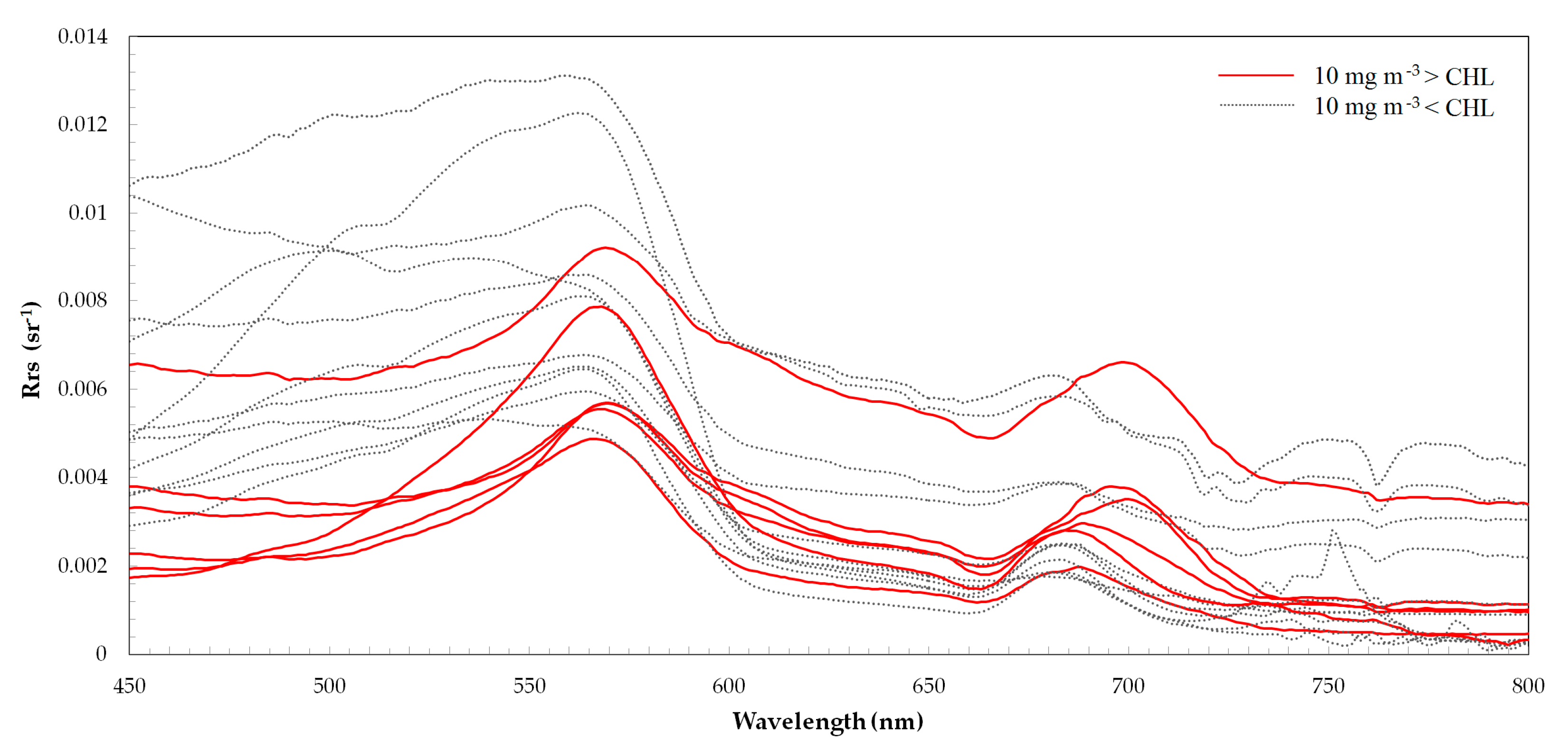
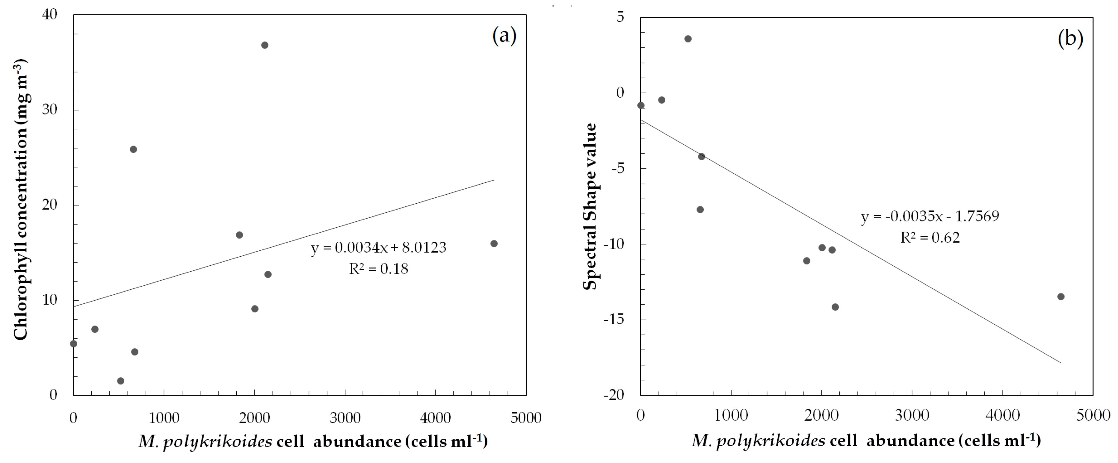
CHL, cell abundance measurements, and the spectra of surface waters taken at 14 sampling locations during the M. polykrikoides bloom period on 7 and 8 August 2018 are shown in Table 4. CHL ranged from 1.5 to 36.8 mg m−3. At two stations (R09 and R10), CHL was very high. The maximum M. polykrikoides cell abundance was 4647 cells mL−1, observed at station R06 in Yeosu. The minimum cell abundance occurred at station Y02 in Namhae, where no M. polykrikoides bloom occurred. For the five other stations (R05, R06, R08, R09, and Y03), M. polykrikoides cell abundances were greater than 1000 cells mL−1. All of these stations are located along Bangjukpo Beach in Yeosu. In situ Rrs patterns at several sampling locations were measured during this field survey. The spectrum displayed peaks near 570 nm and 710 nm, as shown in Figure 2. These patterns indicated the fluorescence properties of phytoplankton. The spectra when CHL was 10 mg m−3 or greater showed a distinct reverse triangle pattern in the green and red wavelengths. When CHL was very high and cell abundance was >2000 cells mL−1, as observed at station R09 (14:00 on 8 August, CHL at 35.8 mg m−3, cell abundance at 2152 cell mL−1), Rrs spectra exhibited patterns typical of M. polykrikoides patches, with lower reflectance at short wavelengths and increased reflectance at green wavelengths. As shown in Figure 3, M. polykrikoides cell abundances had a low correlation (R2 = 0.18) with CHL but a high correlation (R2 = 0.62) with Spectral Shape value estimated from the spectra at 443, 490, and 570 nm for each sampling location.
3.2. Spectral Analysis of M. polykrikoides Using Multi-Sensor Data
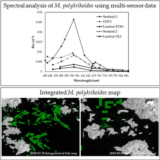
Figure 4 shows M. polykrikoides spectra based on various sensor data. On 29 July 2018, red tide patches of M. polykrikoides were observed near Goheung (Figure 5). Areas with high-density red tides were used for spectral analysis of M. polykrikoides. Rrs spectra collected by five sensors from similar locations at nearly the same time (within 60 min) on the same day showed similar patterns. Rrs spectra showed lower reflectance at short wavelengths and increased reflectance at green wavelengths, similar to the in situ spectrum. These properties appeared in Case-2 waters, which had high levels of SPM and CDOM, and also represent the typical spectrum of M. polykrikoides patches. Spectral Shape algorithm was based on these spectral properties, and can detect M. polykrikoides from the slope changes in the 443–490 nm and 490–555 nm regions. As shown in Figure 4, except for Landsat ETM+, the other four sensors have all the bands used in Spectral Shape algorithm. Morever, the blue bands of GOCI and Sentinel-3 OLCI are composed of multiple subdivisions, while terrestrial sensors have a simple blue band. Comparing the red tide spectra detected by five sensors, ocean color sensor data were more sensitive than terrestrial sensor data. In particular, Sentinel-3 OLCI showed a steep slope in Rrs value for bands used in Spectral Shape algorithm due to its high SNR and spectral resolution.
3.3. Visual Inspection and Comparison
Visual inspection was performed to confirm the red tide patches detected by each sensor. Red tide patches caused by M. polykrikoides usually appear reddish or brown in Rrs true-color composite images. Hence, we could detect red tide areas from Rrs true-color composite images collected with various sensors through simple visual inspection. In Spectral Shape image, a negative value is suspected to indicate red tide areas. Threshold values for Spectral Shape images were determined based on visual identification.
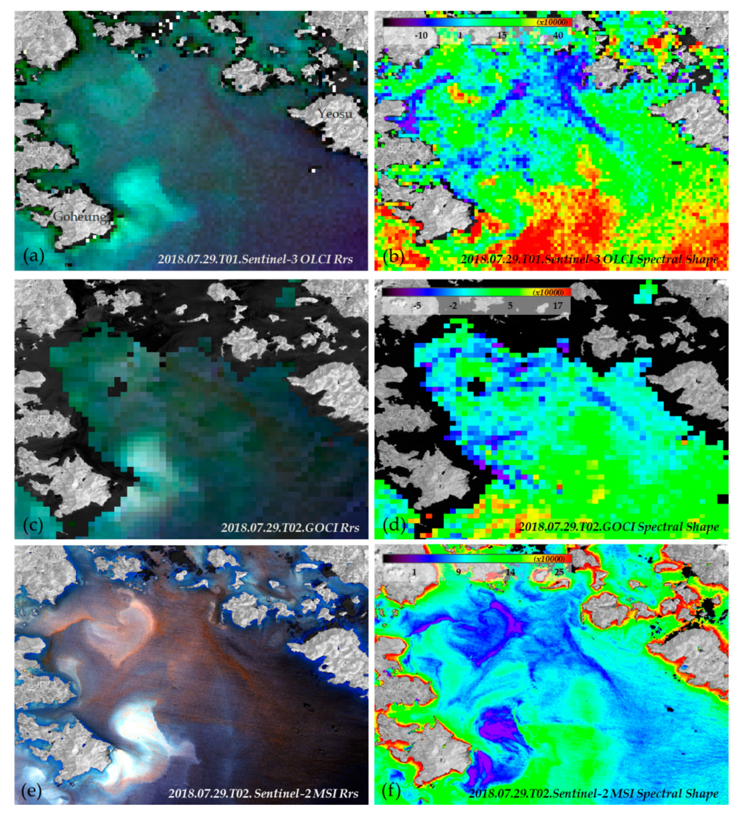
Figure 5 shows Rrs true-color composite and Spectral Shape images based on multi-sensor data collected on 29 July 2018 at Yeosu and Goheung. On the same day, a red tide attention notice for M. polykrikoides was issued from Goheung to Yeosu. In addition, red tide patches appeared sporadically in Bodolbada, while high-density red tide strips appeared in coastal areas of Goheung (2500 cell mL−1). In the Rrs true-color composite and Spectral Shape images of each sensor, red tide patches were observed in similar positions. Moreover, red tide patches that were not detected in the red tide report by NIFS were observed. We calculated red tide coverage by identifying and quantifying red tide patches according to differences in spatial resolution. The red tide coverage estimated from GOCI was 181 pixels × 500 m × 500 m = 45.25 km2. In comparison, the coverage estimated from Sentinel-3 OLCI was 348 pixels × 300 m × 300 m = 31.32 km2, and that estimated from Sentinel-2 MSI was 42,136 pixels × 20 m × 20 m = 16.85 km2. Thus, the ratios of these estimates were GOCI/Sentinel-3 OLCI = 144% and GOCI/Sentinel-2 MSI = 269%, suggesting that GOCI overestimated the red tide coverage by 44% and 169%, respectively, compared with Sentinel-3 OLCI and Sentinel-2 MSI due to its larger pixels.
Figure 6 shows Rrs true-color composite and Spectral Shape images from multi-sensor data collected on 30 July 2018 at Namhae. On the same day, a red tide attention for M. polykrikoides was issued from Goheung to Namhae, and the maximum cell abundance was 700 cell mL−1 along coastal areas of Namhae. Using Sentinel-3 OLCI and Landsat OLI imagery, data can be acquired for the coast of Namhae, as the coast was not masked. However, GOCI was unable to observe this area due to its coarse spatial resolution. Nonetheless, no red tide patches were detected in the Landsat OLI data, perhaps due to the spectral resolution and sensitivity to SNR of the terrestrial sensor being lower than those of ocean color sensor. In addition, we found that GOCI could detect red tide patches, despite having a lower SNR than Sentinel-3 OLCI.
Figure 7 shows another comparison of Sentinel-2 MSI and GOCI imagery for red tide detection. On 1 August 2018, a red tide attention notice for M. polykrikoides was issued from Goheung to Geoje. The maximum cell abundance was 940 cell mL−1 in coastal areas of Yeosu (Figure 8c). Sentinel-2 MSI imagery could be used to detect coastal areas. In contrast, GOCI image was masked in most coastal areas, especially around small islands, due to its low spatial resolution. In addition to the distribution of red tide patches covered by the red tide report, many other red tide patches were detected.
3.4. Integrated Red Tide Map
Figure 8 shows the distribution of red tide patches detected in situ (left) and the integrated red tide map (right) generated from multi-sensor data. The red tide report from NIFS was mainly focused on the coast. Therefore, it contained limited information on red tides occurring outside of the in-situ survey locations. Unlike the red tide report, integrated red tide maps could be used to detect red tide patches near the coast and in the outer sea. On 29 July 2018, the red tide distribution was restricted to coastal areas according to the red tide report. However, the integrated red tide map indicated red tide patches across Bodolbada (Figure 8a,b). Red tide patches were found between islands on 1 August 2018. However, as shown in Figure 7a, detection of red tide patches using GOCI image was difficult (Figure 8c,d) because the coast was masked.
Table 5 lists the red tide areas extracted from multi-sensor data. First, we expected that red tide areas extracted from terrestrial sensor data with high spatial resolution would be larger because most red tides that occurred in the study area were concentrated along the coast. However, when red tide areas extracted from Sentinel-2 MSI and GOCI images were compared, they were overestimated by 169–272% by GOCI compared to Sentinel-2 MSI. This overestimation problem was due to the low spatial resolution of ocean color sensor. In addition, due to the high spectral resolution and SNR, red tide areas that were not detected by the terrestrial sensor might have been detected. Red tide areas estimated from Sentinel-3 OLCI were largest, while those estimated from Landsat OLI were smallest.
3.5. Statistical Assessment
Multi-sensor data collected during the red tide period in 2018 were used for statistical assessment. Confusion matrices and statistical results are summarized in Table 6. Red tide pixels were identified correctly between 0 and 32% of the time. The average FM was 0.15, ranging from 0 to 0.35. The average sensitivity and specificity were 0.14 and 0.89, respectively.
Among single-sensor data, Sentinel-3 OLCI had the highest sensitivity (0.28) and the highest FM (0.35) on 30 July 2018. Sentinel-2 MSI had the highest specificity (0.99). Among multi-sensor data, the highest sensitivity (0.32) was obtained when Sentinel-2 MSI, Sentinel-3 OLCI, and GOCI were combined. On the other hand, the highest FM (0.33) was obtained when Sentinel-2 MSI, GOCI, and Landsat OLI were combined. On 1 August 2018, no red tide pixels were detected at Namhae in GOCI imagery due to coastal area masking, while red tide pixels were detected only with Sentinel-2 MSI. However, a large number of red tide pixels were detected in GOCI image of Yeosu on 1 August 2018, despite being in a coastal area. When Sentinel-2 MSI and GOCI were combined, sensitivity and FM were 183% and 150% higher, respectively, compared to those of GOCI single-sensor data. In four cases, the sensitivity estimated from multi-sensor data was higher than that estimated from a single sensor. FM decreased slightly, except on 1 August 2018, when red tide areas that were not detected in the in-situ survey were much larger than those estimated from sensors.
4. Discussion
Previous studies have reported a relationship between CHL and cell abundance. Tester et al. [14] found that a chlorophyll anomaly of 1 μg L−1 would represent an increase of 105 cells L−1 of K. brevis, and that remote sensing data can detect K. brevis along the Florida coast at concentrations above 50,000 cells L−1. Choi et al. [48] reported that cell abundance and CHL of M. polykrikoides in the East Sea of Korea (ESK) are highly correlated (R2 = 0.99), suggesting that changes in CHL could be determined by changes in M. polykrikoides cell abundance. From calculations based on their observations, one M. polykrikoides cell contained ~73 pg chlorophyll during this bloom period. However, Shin et al. [27] found that estimation of cell abundance from CHL has limitations, as CHL in seawater is determined based on internal chlorophyll content from a mixture of red tide species. Ahn et al. [49] calculated the amount of chlorophyll per cell for red tide species to determine the internal chlorophyll content of each red tide species. M. polykrikoides and Akashiwo sanguinea are red tide species with relatively high internal CHL, while the heterotrophic species Noctiluca scintillans does not have or contains less internal chlorophyll. If red tide species with different internal chlorophyll contents are mixed in the water, it is very difficult to estimate cell abundance from CHL. This relationship is particularly complicated for M. polykrikoides because it coexists with other red tide species in the SSK. In addition, estimation of CHL is a great challenge in waters with complex optical properties [17]. Studies have shown that CHL algorithms that do not consider the influence of SPM can exhibit large errors in turbid waters [50,51]. The waters around the Korean peninsula have diverse optical properties, ranging from relatively clear waters in the East/Japan Sea to extremely turbid waters in coastal regions. Because the ESK has clear water prevailing in chlorophyll, it is possible to estimate cell abundance in that area from CHL, as reported by Choi et al. [48]. In contrast, estimating cell abundance from CHL in the present study area of the SKK was difficult because SPM and CDOM could affect CHL estimation. In fact, the correlation between CHL and cell abundance in this study was low.
Table 6 shows how many false positive (nmr-MR) were obtained. Because the field survey has the limitations of observation areas, it is difficult to find all red tide areas. False positive means the part that was detected from the satellite but not detected from the field survey. In other words, the areas of false positive may be red tide areas that has been detected as false or has not yet been detected in the field survey. It may be used as a complement to the field survey, but it needs to be considered as the red tide suspicious areas. Several factors can reduce the accuracy of statistical assessment for red tide detection using multi-sensor data. Obtaining multi-sensor data collected at the same time is difficult. In this study, we confirmed that the red tide patches moved slightly, despite using images obtained within a maximum of 1 h. Red tide areas extracted from near-coincident multi-sensor data might also differ from the red tide report provided by NIFS. The red tide report is created by summarizing fishermen’s reports and results of a daily field survey for red tide detection [6]. Hence, red tide areas extracted in this study might not represent the red tide distribution for the whole day, as the images used herein were acquired at about 02:00 GMT. Another factor that should be considered in red tide detection is vertical migration of red tide species. Some red tide species migrate vertically according to changes in light, temperature, and nutrients in the water [52]. M. polykrikoides is a relatively slow growing red tide organism. Therefore, it may not be able to outgrow red tide diatoms, flagellates, and other dinoflagellates under the same environmental conditions [7]. However, M. polykrikoides has the ability to swim fast and can theoretically reach 50 m in depth. Thus, it may outgrow other red tide species under conditions of low nutrients and high solar insolation. Some studies have investigated the vertical migration of red tide species using satellite data. Choi et al. [48] found that M. polykrikoides cell abundance was highest at 05:25 GMT by investigating hourly variations in GOCI-derived chlorophyll images. On the other hand, low cell abundances were observed in the early morning and late afternoon. Lou and Hu [25] noted that a P. donghaiense bloom increased from early morning to early afternoon. The bloom size was calculated from MRI using GOCI-derived Rrs. Indeed, GOCI is an optimal sensor for observing vertical migration of red tide species due to its excellent temporal resolution. However, due to its limitation of spatial resolution, it is poor at detecting red tides near the coast. The images used in this study except for GOCI were acquired at about 02:00 GMT, because all sensors are on polar-orbiting satellites with sun-synchronous orbits. Therefore, creating an integrated red tide map representing the entire day from satellite images alone is a great challenge.
SNR and spectral resolution are important factors that determine the red tide detection ability of any sensor. SNR and image quality are highly correlated, and are related to image metrics such as pixel size and edge sharpness [53]. SNR is not constant within an image, but is a function of the scene radiance level [54]. Its performance may drive tradeoffs in terms of the design and cost of the satellite sensor. In general, improved SNR comes at the cost of poorer spatial resolution, lower spectral resolution, less coverage, larger optics, and higher data rate. Ocean color sensors have high SNR and spectral resolution but low spatial resolution compared to terrestrial sensors. On August 1, 2018, a red tide occurred along the coast of Namhae. It was not detected at all by GOCI (Table 6). On the other hand, on 30 July 2018, as shown in Figure 6f, almost no red tide was detected in Landsat OLI, even though the coast was not masked. In other words, when red tide detection is performed using only a single sensor, estimating the overall red tide occurrence area is difficult. SNR is also related to the minimum cell abundance that can be detected in a satellite image. When low cell abundances can be detected by various sensors, it may be possible to improve the red tide warning system by complementing these data with the existing field survey.
5. Conclusions
Damage caused by occurrence of M. polykrikoides in the SSK is particularly great when it is concentrated along the coast. We investigated the synergistic effect of using multi-sensor data to identify M. polykrikoides blooms. The conclusions of this study are as follows.
- (1)
- In the in situ survey, the spectra of samples with 10 mg m−3 or greater CHL showed a distinct reverse triangle pattern in the green and red wavelengths. In situ cell abundance and CHL of M. polykrikoides in the SSK showed low correlations, while Spectral Shape value and cell abundance were highly correlated. This finding implies that the SSK has characteristics of complex waters. Comparing the red tide spectra from near-coincident multi-sensor data, Rrs spectra showed lower reflectance at short wavelength and increased reflectance at green wavelengths, similar to the in situ spectra. Ocean color sensor data were more sensitive than terrestrial sensor data. Specifically, Sentinel-3 OLCI was the most sensitive of the sensors tested.
- (2)
- An integrated red tide map was generated using multi-sensor data. We confirmed the complementary data of red tide patches extracted from each sensor, as well as observations of coastal and offshore areas from the integrated red tide map. The red tide areas estimated from Sentinel-3 OLCI were the most extensive, while those from Landsat OLI were the smallest. This result could be attributed to differences in sensitivity characteristics, such as the spatial resolution, spectral resolution, and SNR of each sensor. A statistical evaluation was conducted to quantitatively assess the synergistic effect of multi-sensor data on the detection of M. polykrikoides. Sensitivity estimated from multi-sensor data was higher than that estimated using a single-sensor, while FM decreased slightly with the use of multi-sensors.
GOCI has superior temporal and spectral resolutions. However, it has limited spatial resolution, complicating detection of M. polykrikoides in coastal areas with complex coastlines. To overcome this limitation, Landsat can be used, which has fine spatial resolution. Unfortunately, its temporal and spectral resolutions are low due to the limitations of the terrestrial sensor. Recently, Sentinel-2 MSI and Sentinel-3 OLCI have been developed, combining the strengths of various resolutions. In particular, Sentinel-3 OLCI has high SNR, high spectral resolution, and wide coverage. It is also suitable for red tide detection due to its spatial resolution of 300 m, which is sufficient to avoid coastal masking. GOCI-2 is scheduled to launch in 2019 with a spatial resolution of 250 m, and could further improve the detection accuracy of red tide areas. The results of this study have enabled us to recognize the synergistic effect on red tide detection of multi-sensor data. Such data can be used to improve the accuracy of red tide detection. Accurate forecasting in conjunction with high-frequency (HF) radar and numerical models may allow for precise estimation of red tide areas and cell abundances. Accurately estimating red tide areas requires observing them with consideration of vertical migration. Therefore, a comprehensive multi-platform approach combining methods such as manned aircraft and unmanned aerial vehicle (UAV) with in situ survey data and satellite data is needed for effective integrated red tide detection.
Author Contributions
Conceptualization, J.S. and J.-H.R.; Field Data Colletion and Experiment, J.S., K.K., and Y.B.S.; Data analysis, J.S. and K.K.; Writing-Original Draft Preparation, J.S.; Writing-Review & Editing, J.S.; Supervision, J.-H.R. and Y.B.S.; Funding Acquisition, J.-H.R.
Funding
This study was supported by “Base research for building a wide integrated surveillance system of marine territory” and “Development of Marine Environmental Monitoring Technology using Remote Sensing –Green tide” funded by the Ministry of Oceans and Fisheries (MOF).
Acknowledgments
The authors would like to thank G.S. Park, D.J. Hwang, and B.J. Kim of KIOST for providing us with field data. We also thank K.Y. Kim of Chonnam National University for his help in analyzing M. polykrikoides cell abundances.
Conflicts of Interest
The authors declare no conflict of interest.
References
- Anderson, D.M.; Alpermann, T.J.; Cembella, A.D.; Collos, Y.; Masseret, E.; Montresor, M. The globally distributed genus Alexandrium: Multifaceted roles in marine ecosystems and impacts on human health. Harmful Algae 2012, 14, 10–35. [Google Scholar] [CrossRef] [PubMed]
- Park, T.G.; Lim, W.A.; Park, Y.T.; Lee, C.K.; Jeong, H.J. Economic impact, management and mitigation of red tides in Korea. Harmful Algae 2013, 30 (Suppl. 1), S131–S143. [Google Scholar] [CrossRef]
- Stumpf, R.P.; Culver, M.E.; Tester, P.A.; Tomlinson, M.; Kirkpatrick, G.J.; Pederson, B.A.; Truby, E.; Ransibrahmanakul, V.; Soracco, M. Monitoring Karenia brevis blooms in the Gulf of Mexico using satellite ocean color imagery and other data. Harmful Algae 2003, 2, 147–160. [Google Scholar] [CrossRef]
- Jeong, H.J.; Yoo, Y.D.; Lee, K.H.; Kim, T.H.; Seong, K.A.; Kang, N.S.; Lee, S.Y.; Kim, J.S.; Kim, S.; Yih, W.H. Red tides in Masan Bay, Korea in 2004–2005: I. Daily variations in the abundance of red-tide organisms and environmental factors. Harmful Algae 2013, 30 (Suppl. 1), S75–S88. [Google Scholar] [CrossRef]
- Gómez, F.; Richlen, M.L.; Anderson, D.M. Molecular characterization and morphology of Cochlodinium strangulatum, the type species of Cochlodinium, and Margalefidinium gen. nov. for C. polykrikoides and allied species (Gymnodiniales, Dinophyceae). Harmful Algae 2017, 63, 32–44. [Google Scholar] [CrossRef]
- Lee, C.K.; Park, T.G.; Park, Y.T.; Lim, W.A. Monitoring and trends in harmful algal blooms and red tides in Korean coastal waters, with emphasis on Cochlodinium polykrikoides. Harmful Algae 2013, 30, S3–S14. [Google Scholar] [CrossRef]
- Jeong, H.J.; Lim, A.S.; Lee, K.; Lee, M.J.; Seong, K.A.; Kang, N.S.; Jang, S.H.; Lee, K.H.; Lee, S.Y.; Kim, M.O.; et al. Ichthyotoxic Cochlodinium polykrikoides red tides offshore in the South Sea, Korea in 2014: I. Temporal variations in three-dimensional distributions of red-tide organisms and environmental factors. Algae 2017, 32, 101–130. [Google Scholar] [CrossRef]
- Forecast∙Breaking News of the National Institute of Fisheries Science (NIFS). Available online: http://www.nifs.go.kr/redtideInfo (accessed on 31 October 2018).
- National Institute of Fisheries Science (NIFS). Harmful Algal Blooms in Korean Coastal Waters; National Institute of Fisheries Science: Busan, Korea, 2015. [Google Scholar]
- Ahn, Y.H.; Shanmugam, P. Detecting the red tide algal blooms from satellite ocean color observations in optically complex Northeast-Asia Coastal waters. Remote Sens. Environ. 2006, 103, 419–437. [Google Scholar] [CrossRef]
- Suh, Y.S.; Jang, L.H.; Lee, N.K.; Ishizaka, J. Feasibility of red tide detection around Korean waters using satellite remote sensing. Fisher Aqua. Sci. 2004, 7, 148–162. [Google Scholar] [CrossRef]
- Tomlinson, M.C.; Wynne, T.T.; Stumpf, R.P. An evaluation of remote sensing techniques for enhanced detection of the toxic dinoflagellate, Karenia brevis. Remote Sens. Environ. 2009, 113, 598–609. [Google Scholar] [CrossRef]
- Tao, B.; Mao, Z.; Lei, H.; Pan, D.; Shen, Y.; Bai, Y.; Zhu, Q.; Li, Z. A novel method for discriminating Prorocentrum donghaiense from diatom blooms in the East China Sea using MODIS measurements. Remote Sens. Environ. 2015, 158, 267–280. [Google Scholar] [CrossRef]
- Tester, P.A.; Stumpf, R.P.; Steidinger, K.A. Ocean color imagery: What is the minimum detection level for Gymnodinium breve blooms. Harmful Algae 1998, 149–151. [Google Scholar]
- Tomlinson, M.C.; Stumpf, R.P.; Ransibrahmanakul, V.; Truby, E.W.; Kirkpatrick, G.J.; Pederson, B.A.; Gabriel, A.V.; Heil, C.A. Evaluation of the use of SeaWiFS imagery for detecting Karenia brevis harmful algal blooms in the eastern Gulf of Mexico. Remote Sens. Environ. 2004, 91, 293–303. [Google Scholar] [CrossRef]
- Son, Y.B.; Kang, Y.H.; Ryu, J.H.; Jeong, J.C. Monitoring red tide in South Sea of Korea (SSK) using the geostationary ocean color imager (GOCI). Korean J. Remote Sens. 2012, 28, 531–548. [Google Scholar] [CrossRef]
- Kim, W.; Moon, J.E.; Park, Y.J.; Ishizaka, J. Evaluation of chlorophyll retrievals from Geostationary Ocean Color Imager (GOCI) for the North-East Asian region. Remote Sens. Environ. 2016, 184, 482–495. [Google Scholar]
- Hu, C.; Muller-Karger, F.E.; Taylor, C.J.; Carder, K.L.; Kelble, C.; Johns, E.; Heil, C.A. Red tide detection and tracing using MODIS fluorescence data: A regional example in SW Florida coastal waters. Remote Sens. Environ. 2005, 97, 311–321. [Google Scholar] [CrossRef] [Green Version]
- Moradi, M.; Kabiri, K. Red tide detection in the Strait of Hormuz (east of the Persian Gulf) using MODIS fluorescence data. Int. J. Remote Sens. 2012, 33, 1015–1028. [Google Scholar] [CrossRef]
- Zhao, J.; Temimi, M.; Ghedira, H. Characterization of harmful algal blooms (HABs) in the Arabian Gulf and the Sea of Oman using MERIS fluorescence data. ISPRS J. Photogramm. Remote Sens. 2015, 101, 125–136. [Google Scholar] [CrossRef]
- Dierssen, H.M.; Kudela, R.M.; Ryan, J.P.; Zimmerman, R.C. Red and black tides: Quantitative analysis of water-leaving radiance and perceived color for phytoplankton, colored dissolved organic matter, and suspended sediments. Limnol. Oceanogr. 2006, 51, 2646–2659. [Google Scholar] [CrossRef] [Green Version]
- Sasaki, H.; Tanaka, A.; Iwataki, M.; Touke, Y.; Siswanto, E.; Tan, C.K.; Ishizaka, J. Optical properties of the red tide in Isahaya Bay, southwestern Japan: Influence of chlorophyll a concentration. J. Oceanogr. 2008, 64, 511–523. [Google Scholar] [CrossRef]
- Cannizzaro, J.P.; Carder, K.L.; Chen, F.R.; Heil, C.A.; Vargo, G.A. A novel technique for detection of the toxic dinoflagellate, Karenia brevis, in the Gulf of Mexico from remotely sensed ocean color data. Cont. Shelf Res. 2008, 28, 137–158. [Google Scholar] [CrossRef]
- Wynne, T.T.; Stumpf, R.P.; Tomlinson, M.C.; Warner, R.A.; Tester, P.A.; Dyble, J.; Fahnenstiel, G.L. Relating spectral shape to cyanobacterial blooms in the Laurentian Great Lakes. Int. J. Remote Sens. 2008, 29, 3665–3672. [Google Scholar] [CrossRef]
- Lou, X.; Hu, C. Diurnal changes of a harmful algal bloom in the East China Sea: Observations from GOCI. Remote Sens. Environ. 2014, 140, 562–572. [Google Scholar] [CrossRef]
- Kim, Y.; Byun, Y.; Kim, Y.; Eo, Y. Detection of Cochlodinium polykrikoides red tide based on two-stage filtering using MODIS data. Desalination 2009, 249, 1171–1179. [Google Scholar] [CrossRef]
- Shin, J.S.; Min, J.E.; Ryu, J.H. A study on red tide surveillance system around the Korean coastal waters using GOCI. Korean J. Remote Sens. 2017, 33, 213–230. [Google Scholar]
- Takahashi, W.; Kawamura, H.; Omura, T.; Furuya, K. Detecting red tides in the eastern Seto inland sea with satellite ocean color imagery. J. Oceanogr. 2009, 65, 647–656. [Google Scholar] [CrossRef]
- Wang, G.; Zhang, B.; Li, J.; Zhang, H.; Shen, Q.; Wu, D.; Song, Y. Study on monitoring of red tide by multi-spectral remote sensing based on HJ-CCD and MODIS. Procedia Environ. Sci. 2011, 11, 1561–1565. [Google Scholar] [CrossRef]
- Oh, S.Y.; Jang, S.W.; Park, W.G.; Lee, J.H.; Yoon, H.J. A comparative Study for Red Tide Detection Methods Using GOCI and MODIS. Korean J. Remote Sens. 2013, 29, 331–335. [Google Scholar] [CrossRef]
- Shin, J.S.; Kim, K.; Ryu, J.H. Red Tide Detection through Image Fusion of GOCI and Landsat OLI. Korean J. Remote Sens. 2018, 34, 377–391. [Google Scholar]
- Jeffrey, S.W.; Humphrey, G.F. New spectrophotometric equations for determining chlorophylls a, b, c1, c2 in higher plants, algae, and natural phytoplankton. Biochem. Physiol. Pflanz. 1975, 167, 191–194. [Google Scholar] [CrossRef]
- Lee, H.G.; Kim, H.M.; Min, J.; Kim, K.; Park, M.G.; Jeong, H.J.; Kim, K.Y. An advanced tool, droplet digital PCR (ddPCR), for absolute quantification of the red-tide dinoflagellate, Cochlodinium polykrikoides Margalef (Dinophyceae). Algae 2017, 32, 189–197. [Google Scholar] [CrossRef]
- Korea Ocean Satellite Center (KOSC). Available online: http://kosc.kiost.ac.kr (accessed on 31 October 2018).
- Ryu, J.H.; Han, H.J.; Cho, S.; Park, Y.J.; Ahn, Y.H. Overview of geostationary ocean color imager (GOCI) and GOCI data processing system (GDPS). Ocean Sci. J. 2012, 47, 223–233. [Google Scholar] [CrossRef]
- Donlon, C.; Berruti, B.; Buongiorno, A.; Ferreira, M.H.; Féménias, P.; Frerick, J.; Goryl, P.; Klein, U.; Laur, H.; Mavrocordatos, C.; et al. The global monitoring for environment and security (GMES) sentinel-3 mission. Remote Sens. Environ. 2012, 120, 37–57. [Google Scholar] [CrossRef]
- European Organisation for Meteorological Satellites (EUMESAT). Available online: https://coda.eumetsat.int (accessed on 31 October 2018).
- U.S. Geological Survey. Available online: http://glovis.usgs.gov (accessed on 18 October 2018).
- Irons, J.R.; Dwyer, J.L.; Barsi, J.A. The next Landsat satellite: The Landsat data continuity mission. Remote Sens. Environ. 2012, 122, 11–21. [Google Scholar] [CrossRef]
- Drusch, M.; Del Bello, U.; Carlier, S.; Colin, O.; Fernandez, V.; Gascon, F.; Hoersch, B.; Isola, C.; Laberinti, P.; Martimort, P.; et al. Sentinel-2: ESA’s Optical High-Resolution Mission for GMES Operational Services. Remote Sens. Environ. 2012, 120, 25–36. [Google Scholar] [CrossRef]
- Copernicus Open Access Hub. Available online: https://scihub.copernicus.eu (accessed on 31 October 2018).
- Brockmann, C.; Doerffer, R.; Peters, M.; Kerstin, S.; Embacher, S.; Ruescas, A. Evolution of the C2RCC neural network for Sentinel 2 and 3 for the retrieval of ocean colour products in normal and extreme optically complex waters. In Proceedings of the Living Planet Symposium, Prague, Czech Republic, 9–13 May 2016. [Google Scholar]
- Chen, J.; Zhu, X.; Vogelmarnn, J.E.; Gao, F.; Jin, S. A simple and effective method for filling gaps in Landsat ETM+ SLC-off images. Remote Sens. Environ. 2011, 115, 1053–1064. [Google Scholar] [CrossRef]
- Carvalho, G.A.; Minnett, P.J.; Banzon, V.F.; Baringer, W.; Heil, C.A. Long-term evaluation of three satellite ocean color algorithm for identifying harmful algal blooms (Karenia brevis) along the west coast of Florida: A matchup assessment. Remote Sens. Environ. 2011, 115, 1–18. [Google Scholar] [CrossRef] [PubMed]
- Ryan, J.P.; Fischer, A.M.; Kudela, R.M.; Gower, J.F.; King, S.A.; Marin, R.; Chavez, F.P. Influences of upwelling and downwelling winds on red tide blooms dynamics in Monterey Bay, California. Cont. Shelf Res. 2009, 29, 785–795. [Google Scholar] [CrossRef]
- Soto, I.M.; Cannizzaro, J.; Muller-Karger, F.E.; Hu, C.; Wolny, J.; Goldgof, D. Evaluation and optimization of remote sensing techniques for detection of Karenia brevis blooms on the West Florida Shelf. Remote Sens. Environ. 2015, 170, 239–254. [Google Scholar] [CrossRef]
- Kohavi, R. Glossary of terms. Mach. Learn. 1998, 30, 127–132. [Google Scholar]
- Choi, J.K.; Min, J.E.; Noh, J.H.; Han, T.H.; Yoon, S.; Park, Y.J.; Moon, J.E.; Ahn, J.H.; Ahn, S.M.; Park, J.H. Harmful algal bloom (HAB) in the East Sea identified by the Geostationary Ocean Color Imager (GOCI). Harmful Algae 2014, 39, 295–302. [Google Scholar] [CrossRef]
- Ahn, Y.H.; Moon, J.E.; Seo, W.C.; Yoon, H.J. Inherent Optical Properties of Red Tide Algal for Ocean Color Remote Sensing Application. J. Korean Soc. Mar. Environ. Eng. 2009, 12, 47–54. [Google Scholar]
- Woźniak, S.B.; Stramski, S.B. Modeling the optical properties of mineral particles suspended in seawater and their influence on ocean reflectance and chlorophyll estimation from remote sensing algorithms. Appl. Opt. 2004, 43, 3489–3503. [Google Scholar] [CrossRef] [PubMed]
- McKee, D.; Cunningham, A.; Wright, D.; Hay, L. Potential impacts of nonalgal materials on water-leaving sun induced chlorophyll fluorescence signals in coastal waters. Appl. Opt. 2007, 46, 7720–7729. [Google Scholar] [CrossRef] [PubMed]
- Schofield, O.; Kerfoot, J.; Mahoney, K.; Moline, M.; Oliver, M.; Lohrenz, S.; Kirkpatrick, G. Vertical migration of the toxic dinoflagellate Karenia brevis and the impact on ocean optical properties. J. Geophys. Res. Oceans 2006, 111, C06009. [Google Scholar] [CrossRef]
- Leachtenauer, J.C.; Malila, W.; Irvine, J.; Colburn, L.; Salvaggio, N. General image-quality equation: GIQE. Appl. Opt. 1997, 36, 8322–8328. [Google Scholar] [CrossRef]
- Schott, J.R.; Gerace, A.; Woodcock, C.E.; Wang, S.; Zhu, Z.; Wynne, R.H.; Blinn, C.E. The impact of improved signal-to-noise ratios on algorithm performance: Case studies for Landsat class instruments. Remote Sens. Environ. 2016, 185, 37–45. [Google Scholar] [CrossRef]
Figure 1.
The study area used for identification of synergistic effects of multi-sensor data. Red dots indicate in situ sampling locations where chlorophyll concentration (CHL), the spectrum of surface waters, and cell abundance were measured. Images from various sensors were obtained on (a) 29 July 2018, (b) 30 July 2018, and (c) 1 August 2018.

Figure 2.
In situ Rrs spectra at all sampling locations. The spectra of samples with 10 mg m−3 or greater CHL show a distinct reverse triangle pattern in the green and red wavelengths.
Figure 2.
In situ Rrs spectra at all sampling locations. The spectra of samples with 10 mg m−3 or greater CHL show a distinct reverse triangle pattern in the green and red wavelengths.

Figure 3.
(a) Correlation between M. polykrikoides cell abundance and CHL, (b) correlation between M. polykrikoides cell abundance and Spectral Shape value.
Figure 3.
(a) Correlation between M. polykrikoides cell abundance and CHL, (b) correlation between M. polykrikoides cell abundance and Spectral Shape value.

Figure 4.
M. polykrikoides spectra based on data from various sensors such as (a) GOCI (b) Sentinel-2 MultiSpectral Instrument (MSI) (c) Sentinel-3 Ocean and Land Colour Instrument (OLCI) (d) Landsat ETM+ (e) Landsat OLI, and (f) five sensors. On 29 July 2018, red tide patches of M. polykrikoides were observed near Goheung. Areas with high-density red tides were sampled for spectral analysis. Comparing the red tide spectra detected by five sensors, ocean color sensors are more sensitive than terrestrial sensors.

Figure 5.
Rrs true-color composite and Spectral Shape images from various sensors on 29 July 2018 at Bodolbada. (a) Sentinel-3 OLCI Rrs true-color composite image (R: 681.25 nm; G: 560 nm; B: 442.5 nm), (b) Sentinel-3 OLCI Spectral Shape image, (c) GOCI Rrs true-color composite image (R: 680 nm; G: 555 nm; B: 490 nm), (d) GOCI Spectral Shape image, (e) Sentinel-2 MSI Rrs true-color composite image (R: 680 nm; G: 560 nm; B: 490 nm), (f) Sentinel-2 MSI Spectral Shape image.

Figure 6.
Rrs true-color composite and Spectral Shape images collected by various sensors on 30 July 2018 at Namhae. (a) Sentinel-3 OLCI Rrs true-color composite image (R: 681.25 nm; G: 560 nm; B: 442.5 nm), (b) Sentinel-3 OLCI Spectral Shape image, (c) GOCI Rrs true-color composite image (R: 680 nm; G: 555 nm; B: 490 nm), (d) GOCI Spectral Shape image, (e) Landsat OLI Rrs true-color composite image (R: 680 nm; G: 561 nm; B: 483 nm), (f) Landsat OLI Spectral Shape image.

Figure 7.
Rrs true-color composite and Spectral Shape images collected with various sensors on 1 August 2018. (a) GOCI Rrs true-color composite image (R: 680 nm; G: 555 nm; B: 490 nm), (b) GOCI Spectral Shape image, (c) Landsat OLI Rrs true-color composite image (R: 680 nm; G: 561 nm; B: 483 nm), (d) Landsat OLI Spectral Shape image.

Figure 8.
Results of the integrated red tide map. (a) Red tide report from National Fisheries Research and Development Institute (NFRDI) on 29 July 2018, (b) integrated red tide map of Bodolbada on 29 July 2018, (c) Red tide report from NFRDI on 1 August 2018, (d) integrated red tide map of Yeosu on 1 August 2018.


Table 1.
Specifications of satellite data used in this study, including data collected with GOCI, Sentinel-3 OLCI, Sentinel-2 MSI and Landsat OLI.
Table 1.
Specifications of satellite data used in this study, including data collected with GOCI, Sentinel-3 OLCI, Sentinel-2 MSI and Landsat OLI.
| Sensor | Spatial Resolution | Swath | Revisit Period | Spectral Range |
|---|---|---|---|---|
| GOCI | 500 m | 2500 km | 8 times/day | 412–865 nm |
| Sentinel-3 OLCI | 300 m | 1270 km | 1–3 days | 400–1020 nm |
| Sentinel-2 MSI | 10 m/20 m/ 60 m | 290 km | 3–5 days | 443–2190 nm |
| Landsat ETM+ | 30 m | 185 km | 16 days | 483–2350 nm |
| Landsat OLI | 30 m | 180 km | 16 days | 443–2290 nm |
Table 2.
Comparison of wavelength, spectral resolution, and SNR among sensors.
| GOCI/Sentinel-3 OLCI | Sentinel-2 MSI/Landsat OLI/ETM+ | |||||
|---|---|---|---|---|---|---|
| Wavelength (nm) | Spectral Resolution (nm) | SNR | Wavelength (nm) | Spectral Resolution (nm) | SNR | |
| Blue1 | 443/443 | 20/10 | 1090/1811 | 443/443/- | 20/15/- | 129/237/- |
| Blue2 | 490/490 | 20/10 | 1170/1541 | 490/482/483 | 65/60/60 | 154/367/39 |
| Green | 555/560 | 20/10 | 1070/1280 | 560/561/561 | 35/57/80 | 168/304/37 |
Table 3.
List of available satellite images of the South Sea of Korea (SSK) during the red tide bloom event in 2018.
Table 3.
List of available satellite images of the South Sea of Korea (SSK) during the red tide bloom event in 2018.
| July 2018 | August 2018 | ||||||||||||||||
| day | 24 | 25 | 26 | 27 | 28 | 29 | 30 | 31 | 1 | 2 | 3 | 4 | 5 | 6 | 7 | 8 | 9 |
| GOCI | |||||||||||||||||
| S3A | |||||||||||||||||
| S2-YS | |||||||||||||||||
| S2-TY | |||||||||||||||||
| L-YS | |||||||||||||||||
| L-TY | |||||||||||||||||
1 S3A: Sentinel-3 OLCI, S2-YS: Sentinel-2 MSI at Yeosu, S2-TY: Sentinel-2 MSI at Tongyeong, L-YS: Landsat at Yeosu, L-TY: Landsat at Tongyeong.
Table 4.
In situ measurements of CHL and Margalefidinium cell abundance at each sampling location in the study area (Spectral Shape value was estimated from the spectra at 443, 490, and 570 nm for each sampling location).
Table 4.
In situ measurements of CHL and Margalefidinium cell abundance at each sampling location in the study area (Spectral Shape value was estimated from the spectra at 443, 490, and 570 nm for each sampling location).
| St. ID | Time | Chlorophyll (mg m−3) | Cell Abundance (cells mL−1) | Spectral Shape Value |
|---|---|---|---|---|
| R01 | 7 August 2018 12:11 | 6.1 | - | 0.8 |
| R02 | 7 August 2018 14:25 | 8.2 | - | −1.7 |
| R03 | 7 August 2018 15:15 | 4.1 | - | 4.2 |
| R04 | 8 August 2018 11:37 | 1.5 | 526 | 3.6 |
| R05 | 8 August 2018 12:54 | 16.9 | 1836 | −11.1 |
| R06 | 8 August 2018 12:59 | 15.9 | 4647 | −13.5 |
| R07 | 8 August 2018 13:12 | 4.58 | 678 | −4.2 |
| R08 | 8 August 2018 13:18 | 12.7 | 2152 | −14.2 |
| R09 | 8 August 2018 14:00 | 36.8 | 2115 | −10.4 |
| R10 | 8 August 2018 14:24 | 25.9 | 663 | −7.7 |
| Y01 | 8 August 2018 11:29 | 1.5 | 0.1 | 18.1 |
| Y02 | 8 August 2018 13:35 | 7.4 | 237 | −0.5 |
| Y03 | 8 August 2018 14:20 | 9.1 | 2005 | −15 |
| Y04 | 8 August 2018 15:28 | 5.4 | 5 | −0.8 |
Table 5.
Red tide areas extracted from multi-sensor data.
| Date | Region | Sensor | Area (km2) | Per. (%) | Date | Region | Sensor | Area (km2) | Per. (%) |
|---|---|---|---|---|---|---|---|---|---|
| 29 July 2018 | Yeosu Goheung | S2 | 7.2 | 20.8 | 30 July 2018 | Namhae | S3 | 7.8 | 83.3 |
| G | 12.2 | 35.3 | G | 2.5 | 26.5 | ||||
| S3 | 16.6 | 47.9 | LC8 | 0.7 | 7.9 | ||||
| S2+G+S3 | 34.7 | 100 | S3+G+LC8 | 9.3 | 100 | ||||
| 1 August 2018 | Namhae | S2 | 4.4 | 39.3 | 1 August 2018 | Yeosu | S2 | 2.5 | 27 |
| G | 7.2 | 64.1 | G | 6.8 | 73.6 | ||||
| G+S2 | 11.2 | 100 | G+S2 | 9.3 | 100 |
1 S2: Sentinel- MSI, S3: Sentinel-3 OLCI, G: GOCI, LC8: Landsat OLI.
Table 6.
Performance evaluation of each sensor for Yeosu, Goheung, and Namhae.
| Date | Region | Sensor | mr-MR | mr-nMR | nmr-MR | nmr-nMR | FM | Sens. | Spec. |
|---|---|---|---|---|---|---|---|---|---|
| 29 July 2018 | Yeosu/Goheung | S2 | 4754 | 19,041 | 13,242 | 1,195,932 | 0.23 | 0.20 | 0.99 |
| G | 268 | 23,527 | 30,307 | 1,178,867 | 0.01 | 0.01 | 0.97 | ||
| S3 | 3197 | 20,598 | 38,365 | 1,170,809 | 0.10 | 0.13 | 0.97 | ||
| S2+G+S3 | 7562 | 16,233 | 79,125 | 1,130,049 | 0.14 | 0.32 | 0.93 | ||
| 30 July 2018 | Namhae | S3 | 8877 | 22,354 | 10,580 | 56,701 | 0.35 | 0.28 | 0.84 |
| G | 280 | 30,951 | 5906 | 61,375 | 0.01 | 0.01 | 0.91 | ||
| LC8 | 167 | 31,064 | 1673 | 65,608 | 0.01 | 0.01 | 0.98 | ||
| S3+G+LC8 | 8947 | 22,284 | 14,404 | 52,877 | 0.33 | 0.29 | 0.79 | ||
| 1 August 2018 | Namhae | S2 | 5179 | 15,377 | 5179 | 15,377 | 0.34 | 0.25 | 0.75 |
| G | 0 | 20,556 | 17,925 | 67,174 | 0.00 | 0.00 | 0.79 | ||
| G+S2 | 5179 | 15,377 | 22,781 | 62,318 | 0.21 | 0.25 | 0.73 | ||
| 1 August 2018 | Yeosu | S2 | 2311 | 50923 | 3933 | 250,410 | 0.08 | 0.04 | 0.98 |
| G | 3347 | 49887 | 13,691 | 240,652 | 0.10 | 0.06 | 0.95 | ||
| G+S2 | 5619 | 47615 | 17,521 | 236,822 | 0.15 | 0.11 | 0.93 |
1 S2: Sentinel-MSI; S3: Sentinel-3 OLCI; G: GOCI; LC8: Landsat OLI; Sens.: Sensitivity; Spec.: Specificity.
© 2018 by the authors. Licensee MDPI, Basel, Switzerland. This article is an open access article distributed under the terms and conditions of the Creative Commons Attribution (CC BY) license (http://creativecommons.org/licenses/by/4.0/).
Share and Cite
MDPI and ACS Style
Shin, J.; Kim, K.; Son, Y.B.; Ryu, J.-H. Synergistic Effect of Multi-Sensor Data on the Detection of Margalefidinium polykrikoides in the South Sea of Korea. Remote Sens. 2019, 11, 36. https://doi.org/10.3390/rs11010036
AMA Style
Shin J, Kim K, Son YB, Ryu J-H. Synergistic Effect of Multi-Sensor Data on the Detection of Margalefidinium polykrikoides in the South Sea of Korea. Remote Sensing. 2019; 11(1):36. https://doi.org/10.3390/rs11010036
Chicago/Turabian StyleShin, Jisun, Keunyong Kim, Young Baek Son, and Joo-Hyung Ryu. 2019. "Synergistic Effect of Multi-Sensor Data on the Detection of Margalefidinium polykrikoides in the South Sea of Korea" Remote Sensing 11, no. 1: 36. https://doi.org/10.3390/rs11010036
Note that from the first issue of 2016, this journal uses article numbers instead of page numbers. See further details here.