An Improved Spatio-Temporal Adaptive Data Fusion Algorithm for Evapotranspiration Mapping
by
Tong Wang
1,2, 
Ronglin Tang
1,2,*,
Zhao-Liang Li
3,4,
Yazhen Jiang
2,3,
Meng Liu
1,2 and
Lu Niu
1,2 1
State Key Laboratory of Resources and Environment Information System, Institute of Geographic Sciences and Natural Resources Research, Chinese Academy of Sciences, Beijing 100101, China
2
College of Resources and Environment, University of Chinese Academy of Sciences, Beijing 100049, China
3
ICube, UdS, CNRS; 300 Boulevard Sebastien Brant, CS10413, 67412 Illkirch, France
4
Key Laboratory of Agricultural Remote Sensing, Ministry of Agriculture/Institute of Agricultural Resources and Regional Planning, Chinese Academy of Agricultural Sciences, Beijing 100081, China
*
Author to whom correspondence should be addressed.
Remote Sens. 2019, 11(7), 761; https://doi.org/10.3390/rs11070761
Submission received: 25 February 2019
/
Revised: 22 March 2019
/
Accepted: 25 March 2019
/
Published: 29 March 2019
(This article belongs to the Special Issue Remote Sensing of Evapotranspiration (ET))
Abstract
:Continuous high spatio-temporal resolution monitoring of evapotranspiration (ET) is critical for water resource management and the quantification of irrigation water efficiency at both global and local scales. However, available remote sensing satellites cannot generally provide ET data at both high spatial and temporal resolutions. Data fusion methods have been widely applied to estimate ET at a high spatio-temporal resolution. Nevertheless, most fusion methods applied to ET are initially used to integrate land surface reflectance, the spectral index and land surface temperature, and few studies completely consider the influencing factor of ET. To overcome this limitation, this paper presents an improved ET fusion method, namely, the spatio-temporal adaptive data fusion algorithm for evapotranspiration mapping (SADFAET), by introducing critical surface temperature (the corresponding temperature to decide soil moisture), importing the weights of surface ET-indicative similarity (the influencing factor of ET, which is estimated from remote sensing data) and modifying the spectral similarity (the differences in spectral characteristics of different spatial resolution images) for the enhanced spatial and temporal adaptive reflectance fusion model (ESTARFM). We fused daily Moderate Resolution Imaging Spectroradiometer (MODIS) and periodic Landsat 8 ET data in the SADFAET for the experimental area downstream of the Heihe River basin from April to October 2015. The validation results, based on ground-based ET measurements, indicated that the SADFAET could successfully fuse MODIS and Landsat 8 ET data (mean percent error: −5%), with a root mean square error of 45.7 W/m2, whereas the ESTARFM performed slightly worse, with a root mean square error of 50.6 W/m2. The more physically explainable SADFAET could be a better alternative to the ESTARFM for producing ET at a high spatio-temporal resolution.
1. Introduction
Evapotranspiration (ET), including soil evaporation and vegetation transpiration, is defined as the movement of water from the land surface into air and continuously acquiring ET at a high spatio-temporal resolution at field or sub-field scales is of critical significance for agricultural and hydrological cycle modelling, irrigation water efficiency quantification and agricultural water resource management [1]. Satellite remote sensing has already been considered a reliable and efficient tool for monitoring spatially distributed ET over large zones. However, a single satellite cannot provide ET at a high spatio-temporal resolution due to the trade-off between the spatial and temporal resolutions of thermal bands in current satellite sensors. For instance, Landsat series imagery can be used to map ET at a relatively high spatial resolution, while ET dynamics cannot be observed, due to the 16-day revisit interval of a single Landsat platform. In contrast, moderate-resolution sensors, such as the Moderate Resolution Imaging Spectroradiometer (MODIS), provide imagery for ET estimation on a daily basis but the relatively coarse spatial resolution hinders the application of ET for the quantification of irrigation water efficiency and water resource management at field, local or basin scales.
To overcome this limitation, previous studies have proposed several methods, mainly including traditional downscaling methods and data fusion methods [2]. Downscaling methods comprise a scaling process of converting coarse spatial resolution images into finer spatial resolution images; however, these methods cannot simultaneously enhance the temporal resolution of the sensor [3] and have rarely been used in recent years [4,5,6]. Data fusion methods use two or more images to obtain fine spatial resolution images; thus, they can simultaneously improve the spatial resolution and temporal coverage. To date, several data fusion methodologies, which were originally developed to fuse land surface reflectance and spectral index data, have been utilized to attempt the estimation of ET at a fine spatio-temporal resolution from ET at a high spatial resolution and high temporal resolution [7,8,9,10,11,12,13,14,15,16,17,18,19,20,21,22,23,24]. These data fusion methods can be divided into two categories: (1) fuse intermediate variables to estimate ET and (2) fuse ET data. For the first category, ET at a high spatio-temporal resolution is estimated by different ET models using intermediate variables that are closely related to ET, such as the reference ET fraction (ETrF), normalized differential vegetation index (NDVI) and land surface temperature (LST). These intermediate variables can be fused using a regression model [12,25] or different spatio-temporal data fusion models [23,26,27]. For the second category, different spatio-temporal data fusion models are directly applied to fuse ET. For example, Ke et al. [26] and Ma et al. [28] applied the spatial and temporal adaptive reflectance fusion model (STARFM) and the enhanced spatial and temporal adaptive reflectance fusion model (ESTARFM), respectively, to fuse multi-source ET data, while a research group at the U.S. Department of Agriculture (USDA) used the STARFM to fuse ET at the GEOS Imager-derived 3 km–10 km, MODIS 1 km and Landsat 30 m scales from the Atmosphere-Land Exchange Inverse (ALEXI) model and the associated flux disaggregation model (DisALEXI) [7,8,9,10,11,13,18,29,30]. For either the first or second category, the most widely and successfully used spatio-temporal data fusion models are the STARFM and ESTARFM, respectively. However, it should be noted that existing methods also have the following limitations: most fusion methods applied to ET are initially used to integrate the land surface reflectance, spectral index and LST; thus, these methods cannot completely consider the influencing factor of ET including remote sensing and atmospheric characteristics [31] (especially some critical issues, such as soil moisture [32] and vegetation distribution) [33,34].
The objectives of this paper are twofold: (1) to develop a spatio-temporal adaptive data fusion algorithm for evapotranspiration mapping (SADFAET) for producing ET at a fine resolution and (2) to fuse ET using Landsat 8 and MODIS image data and validate the fused ET data with ground-based measured data collected downstream of the Heihe River basin. The SADFAET improves on the original ESTARFM algorithm by introducing the critical surface temperature (the corresponding temperature to decide soil moisture) to select similar pixels, importing the weight for surface ET-indicative similarity (the influencing factor of ET which is estimated from remote sensing data) and modifying the spectral similarity (the differences in spectral characteristics between different spatial resolution images) by incorporating the shortwave infrared bands. Section 2 presents the background and the methodology on how the SADFAET was derived. Section 3 describes the study site, the ground-based meteorological and energy flux measurements, satellite data and data preprocessing. Section 4 provides the results and discussion. The conclusions are finally made in Section 5.
2. Methods
2.1. A Brief Overview of the ESTARFM
The ESTARFM was developed to fuse the land surface reflectance by Zhu et al. [35], which was based on the STARFM [36] and the two methods are the most common remote sensing data fusion methods that obtain fine spatial resolution images on a specified date from coarse spatial resolution images on the same date and one or more additional fine-coarse resolution pair. These methods can accurately predict fine-resolution images for heterogeneous landscapes and are the most common remote sensing data fusion methods. In ESTARFM, unknown fine-resolution reflectance on the predicted date tp can be fused using the known fine-resolution reflectance acquired on the reference date tm (right before tp) and tn (right after tp) together with the corresponding coarse-resolution reflectance on tm, tn and tp by introducing similar pixels (i.e., spectrally similar and homogeneous neighboring pixels within the moving window), a conversion coefficient and a weighting coefficient. Although the ESTARFM and the STARFM were originally designed to produce reflectance data, they were also used to produce high spatial resolution NDVI, LST and ET data [7,8,9,13,18,26,28,37,38]. Similar to the ESTARFM, Weng et al. [3] proposed a spatio-temporal adaptive data fusion algorithm for temperature mapping (SADFAT), corresponding to deriving the ESTARFM by nonlinear methods, which was proven to accurately predict fine-resolution radiance products. Since both reflectance and radiance contribute to the variation in ET and the ESTARFM was proven to accurately fuse reflectance and radiance data, this study developed a spatio-temporal adaptive data fusion algorithm for evapotranspiration mapping (SADFAET) by introducing ET, which has a greater influence, into the ESTARFM.
2.2. Theoretical Basis of the SADFAET
The SADFAET, which improves on the original ESTARFM algorithm by introducing the critical surface temperature (T*) the corresponding temperature when surface soil moisture availability in the upper soil layer for each pixel decreases to 0 and vegetation becomes soil water-stressed, which is defined in the work of Tang & Li [39] to decide soil moisture, importing the weight for surface ET-indicative similarity and modifying the spectral similarity by incorporating the shortwave infrared bands (representing soil moisture), is developed to fuse different spatial-temporal resolution ET products to estimate fine-resolution ET data. In the SADFAET, the calculation of fine-resolution ET is modified from that of the ESTARFM algorithm and the ET over a fine-resolution pixel at the prediction time can be calculated by the sum of the fine-resolution ET data at the reference time and coarse-resolution ET data at the reference and prediction times. Similar to the ESTARFM, the moving window is used to search similar pixels within the window and information of similar pixels is then integrated into fine-resolution ET calculation. Unknown fine-resolution ET data of the central pixel (xw/2, yw/2) on the predicted date tp in the SADFAET can be computed using the known fine-resolution ET data acquired on the reference date tm and tn together with the corresponding coarse-resolution ET data on tm, tn and tp:
where the subscript C represents the coarse-resolution pixel and the subscript F represents the fine-resolution pixel. w represents the side length of the moving window, which is used to search similar pixels and is determined by the spatial resolution of the input image. The co-ordinate location of the similar pixel is (i, j) and (w/2, w/2) is the coordinate location of the central pixel. Wi,j,tk represents the weight of the similar pixel computed from the surface ET-indicative similarity, the improved spectral similarity and the distance weight between the similar pixel and the central pixel. Vi,j,tk represents the conversion coefficient of the similar pixel, which can be obtained by linear regression analysis for each similar pixel on the reference date tm and tn [35]. Tk represents the temporal weight. The operator Γ(X) represents .
There are 4 major steps, including the selection of similar neighboring pixels, the calculation of the weights of similar pixels, the calculation of the conversion coefficient and the calculation of the temporal weight for ET fusion. The SADFAET improves the selection of similar neighboring pixels and the calculation of the weight of similar pixels but follows the work of Zhu et al. [35] to determine the window size, temporal weight and conversion coefficient.
2.2.1. Selection of Similar Neighboring Pixels
According to the original ESTARFM models, two methods were used to obtain similar pixels, including the setting threshold and unsupervised classification. However, these two methods mainly consider spectral similarity rather than the ET similarity between the central pixel and other pixels within the search window, while the number of classes limits the automated fusion processing and reduces the accuracy of the similar pixel selection. Note that soil moisture is an important environmental factor that can significantly influence ET. In the SADFAET, the new method is therefore to take into account soil moisture in order to select similar neighboring pixels more reasonably by first introducing a critical surface temperature (T*) and then judging how T* and the remotely sensed surface temperature vary. The T* corresponds to the surface temperature when the surface soil moisture availability in the upper soil layer decreases to 0 and the vegetation becomes soil water-stressed [39] and it can be estimated using the theoretical surface temperature at 2 hypothesized end-members, Tsd with no soil water availability at the upper layer and with zero evaporation and Tvw with well-watered vegetation with potential transpiration, from the following equations.
where Tsd and the Tvw represent the theoretical surface temperature of the dry soil and well-watered vegetation, respectively. Cp represents the specific heat capacity at constant pressure (J/(m·K)). ρ represents the density of air (kg/m3). Δ represents the slope of saturated vapor pressure versus air temperature (kPa/°C). VPD represents the vapor pressure deficit of the air (kPa). Ta represents the near-surface air temperature (K). γ represents the psychrometric (kPa/°C). rvw represents the canopy resistances at the well-watered vegetation (s/m). ras represents the aerodynamic resistance at dry soil (s/m).
When the actual LST (retrieved by remote sensing) for the pixel is lower than or equal to T*, the vegetation component is considered to be potentially transpiring and the soil component is considered to be evaporating at a rate between zero and its maximum value (i.e., the potential rate); otherwise, no water is available to be evaporated for the soil component and the vegetation component transpires with a certain degree of soil water stress. Below are the procedures of the proposed method for selecting similar pixels.
- (1).
- For each fine-resolution pixel at tm and tn, record T* and the LST retrieved from remote sensing data (TR).
- (2).
- For a given pixel, if the remotely sensed TR at a fine resolution at tm is equal to or greater than T* and TR at tn is equal to or greater than T* as well, this pixel is considered to fall into CLASS 1, where no water is available to be evaporated for the soil component and the vegetation component transpires with a certain degree of soil water stress between tm and tn.
- (3).
- If TR at tm is greater than T* but TR at tn is less than T* at the same time, this pixel is considered to fall into CLASS 2, where the surface soil moisture is increasing, and the vegetation transpiration is increasing to the potential transpiration amount between tm and tn.
- (4).
- If TR at tm is less than T* but TR at tn is greater than T* at the same time, the pixel is considered to fall into CLASS 3, where the surface soil moisture decreases to zero while the vegetation component transpires from a maximum value (i.e., the potential transpiration) to a certain degree of soil water stress between tm and tn.
- (5).
- If TR at tm is less than T* and TR at tn is less than T* as well, this pixel is considered to fall into CLASS 4, where the vegetation component transpires potentially, and the surface soil moisture is between zero and a maximum value between tm and tn.
- (6).
- Finally, compare the class (CLASS 1 through CLASS 4) of the central pixel with the given neighboring pixel. If the two pixels fall into the same class, the given neighboring pixel is considered to be a similar neighboring pixel.
2.2.2. Calculation of the Weight of the Similar Pixel
After finishing the selection of a similar pixel, its weight (W) is calculated. However, the original W cannot completely represent the ET; thus, Wi is modified in this paper and the improved weight is computed from the spectral similarity, the surface ET-indicative similarity and the distance between the similar pixel and the central pixel in the SADFAET.
Calculations of the spectral similarity need to consider the effects of surface soil moisture and several indices derived from optical remote sensing observations have been proposed for measuring soil moisture [40], such as the Shortwave Infrared Water Stress Index (SIWSI) [41], the Shortwave-infrared Perpendicular Drought Index (SPDI) [42] and the Visible and Shortwave-infrared Drought Index (VSDI) [43]. We can see that all of these indices use shortwave infrared bands. However, in the ESTARFM and SADFAT, the spectral similarity is calculated using only shortwave and thermal infrared bands; thus, we make an improvement to introduce the shortwave infrared bands into the calculation of spectral similarity to indicate the changes in soil moisture and ET. Here, the spectral similarity (Si,j,tk) is determined by the correlation coefficient of the spectral vector, including shortwave bands (representing vegetation cover), shortwave infrared bands (representing soil moisture) and thermal infrared bands (representing LST), between each similar pixel and its corresponding coarse-resolution pixel with the following equations:
where Fijk and Cijk represent the coarse and fine spatial resolution image spectral vectors respectively at tk, including the reflectance of shortwave infrared bands (BSWIR), shortwave bands (BS) and the radiance of thermal infrared bands (BNIR). For example, with the Landsat 8 data in this study, the BS covers bands 2–5 (blue, green, red and NIR, respectively), BSWIR covers bands 6 and 7 (SWIR 1 and 2, respectively) and the BNIR covers bands 10 and 11 (TIRS 1 and 2, respectively). E() represents the expected value and D() represents the variance value. Combining SWIR information can introduce soil moisture into the fusion model and improve the accuracy of fused ET data.
The surface ET indicators include NDVI, LST, soil moisture and ET [44,45]. We can calculate the changes in surface ET indicators for both the central pixel and the selected similar pixel between tm and tn and determine the weights of different similar pixels to avoid the influence of the selected useless pixel. The weight for the surface ET-indicative similarity of the ith similar pixel (WSCi,j,tk) can be calculated from the correlation coefficient of the surface ET indicator vector as follows:
where the subscripts “central” represent central pixels, respectively. SM represents the soil moisture.
The weight of a similar pixel (Wi,j,tk) is calculated can be given as follows:
where Si,j,tk represents the spectral similarity between fine- and coarse-resolution pixels for the similar pixels (i, j). WSCi,j,tk represents the weight of the surface ET-indicative similarity between the similar pixels (i, j) and central pixel (w/2, w/2). di,j,tk represents the geographic distance between the ith similar pixel and central pixel.
Figure 1 presents a schematic diagram of the SADFAET. This algorithm requires two pairs of fine- and coarse-resolution images on the same date and a set of coarse-resolution images for the prediction dates. Before implementing the SADFAET, the fine-resolution LST, NDVI, soil moisture and ET data at the reference time must be retrieved. There are 6 major steps in the SADFAET implementation. First, fine-resolution LST and T* data are used to select similar neighboring pixels. Second, the fine- and coarse-resolution shortwave infrared bands, the shortwave bands and the radiance in the thermal infrared bands are used to calculate the spectral similarity. Third, surface ET-indicative similarity is estimated by fine-resolution LST, NDVI, soil moisture and ET data. Fourth, the geographic distance and temporal weight are calculated. Fifth, the conversion coefficient is determined by linear regression. Finally, the above weight, similarity and coefficient are used to calculate the ET at a fine resolution at the predicted time.
2.3. End-Member-Based Soil and Vegetation Energy Partitioning Model
The end-member-based soil and vegetation energy partitioning (ESVEP) model [39] was developed for estimating soil and vegetation ET from remote sensing data by considering the differing responses of the soil water content in the upper surface layer to soil evaporation and those in the deeper root zone layer to vegetation transpiration. This model defines four hypothesized end-members, including dry soil (i.e., no soil water availability in the upper layer and zero evaporation), dry vegetation (i.e., no soil water availability and zero transpiration), wet soil (i.e., potential evaporation) and well-watered vegetation (i.e., potential transpiration). Based on the difference in vegetation height in different partially vegetated pixels, four end-member temperatures can be estimated pixel-by-pixel. The actual surface temperature for the partially vegetated pixel consequentially falls between the maximum and minimum of its hypothesized end-member temperature. When the vegetation temperature and energy are separated from their soil components, the ESVEP abides by two principles: (1) when soil evaporation is greater than zero, the vegetation transpiration equals the maximum (potential transpiration) and (2) when vegetation is soil-water stressed, the soil evaporation equals zero.
There are three major steps in the ESVEP model implementation. First, a physical algorithm [46] is used to estimate the divergence in the surface net radiation and soil heat flux. Second, the theoretical surface temperature at each of the four hypothesized end-members is calculated by the surface energy balance equation and the Penman–Monteith equation. Finally, when the actual LST (retrieved by remote sensing) for the pixel is lower than or equal to the critical surface temperature, as presented in Equation (7), the vegetation component is considered to be potentially transpiring and the soil component is considered to be evaporating at a rate between zero and the maximum value (i.e., the potential rate). The vegetation and soil component latent heat flux (LEv and LEs, respectively) under this condition are estimated as:
where Ts and Tsw represent the soil component temperature and theoretical surface temperature of the saturated soil, respectively. LEvw and LEsw represent the theoretical latent heat flux in the well-watered vegetation and saturated soil, respectively.
Otherwise, when no water is available to be evaporated in the soil component and the vegetation component transpires with a certain degree of soil water stress, the LEv and LEs are estimated as:
where Tv and Tvd represent the vegetation component temperature and the theoretical surface temperature of dry vegetation, respectively. LEsd represents the theoretical LE of the dry soil.
The ESVEP model is demonstrated to be no more sensitive to meteorological, vegetation and remote sensing inputs than other ET models and has great potential for producing reasonably good surface energy fluxes. In our study, the fine- and coarse-resolution ET data at the reference time and the fine-resolution ET data at the prediction time were estimated by the ESVEP model [39].
2.4. Validation of the SADFAET
The SADFAET algorithm was applied to the actual Landsat 8 and MODIS images, which aided in understanding its accuracy and reliability. To avoid the impact of ET retrieval, the accuracy of the ET estimates from the ESVEP was first evaluated. The performance of the SADFAET was then assessed through retrieved ET from Landsat 8 data and ground-based measurements. The mean, maximum and minimum ET, standard deviation and histogram of differences of SADFAET and Landsat 8 ET were also used to validate the spatial patterns of fused ET. The fused ET was further compared with the ground-based eddy covariance (EC) measurement to validate the accuracy of the SADFAET based on the mean bias (MB), mean percent error (MPE) and root mean square error (RMSE). The MPE can be calculated as:
where Bi represents the bias of the ith datum. Oi represents the observation of the ith data. N represents the number of data.
3. Materials
3.1. Test Sites and Ground-Based Data
The study area is downstream of the Heihe River basin (LU: 42.0333°N, 101.1°E, RL: 41.9667°N, 101.1667°E), which is an endorheic basin located in the arid and semiarid regions of Northwest China. The annual mean temperature, relative humidity and wind speed are 9.4 °C, 33.7% and 3.2 m/s, respectively and the annual precipitation is approximately 50 mm. There are five ground sites, namely, Sidaoqiao, Populus euphratica, Mixed Forest, Barren land and Cropland, in the study area and the landscapes are comprised of Tamarix, populus euphratica, Populus euphratica and Tamarix, bare land and melon, respectively (Table 1 & Figure 2). Ground-based half-hourly average atmospheric variables (air temperature, wind speed, atmospheric pressure and relative humidity) and downward solar radiation, which were collected from April 2015 to October 2015 at the five ground sites, are used for this study and can be obtained from the Heihe Integrated Observatory Network (http://www.heihedata.org/) [47,48]. The EC system and a large aperture scintillometer (LAS) provided the measurements of turbulent fluxes downstream of the Heihe River basin, while the sample frequencies are 10 Hz (for EC) and 1 min (for LAS) and the heights are 3.5 m (for EC at the Cropland and Barren Land sites), 22 m (for EC at the Mixed Forest and Populus euphratica sites), 8 m (for EC at the Sidaoqiao site) and 22.5 m (for LAS). The LAS and EC flux data were processed and screened according to the criteria suggested in Liu et al. [47]. The instantaneous ET was validated by using 10-min flux measurements as ground-truth data.
3.2. Satellite Data
Multi-source remote sensing data at different spatial and temporal resolutions were obtained from Landsat 8 and Terra MODIS (Table 2). The spatial resolutions of Landsat 8 and MODIS are 30 m and 500–1000 m, respectively, while the temporal resolutions are 8–16 days and 1 day, respectively. Fifteen predominantly clear scenes (day of year [doy]: 96, 103, 135, 144, 160, 176, 199, 215, 231, 240, 247, 256, 288, 295 and 304) of Landsat 8 data from Path 133, Row 31 and Path 134, Row 31 acquired for the period of April to October 2015 were collected from the United States Geological Survey (USGS) (https://landsat.usgs.gov/). The shortwave reflectance band and the thermal band of the 15 scenes were atmospherically corrected using the ENVI. The corresponding MODIS (Terra) datasets, including the 1 km calibrated radiance product (MOD021KM), geolocation product (MOD03), precipitable water product (MOD05_L2), surface reflectance product (MOD09GA), land surface temperature/emissivity product (MOD11A1) and vegetation index product (MOD13A2), were obtained from the Land Processes Distributed Active Archive Center (LP DAAC) (http://glovis.usgs.gov/).
Before the implementation of the SADFAET, both Landsat 8 (OLI/TIRS) and MODIS data need to be calibrated over the same coordinate system (Universal Transverse Mercator projection, UTM) and resampled at the same spatial resolution (30 m). MODIS Reprojection Tools (MRTs) were used to resample and re-project the MODIS data to the Landsat resolution and extent. Landsat 8 data were calibrated and atmospherically corrected for the shortwave reflectance band using the ENVI. Considering the landscape and land cover types of this area, the size of the search window was set as 30 Landsat 8 pixels.
Based on the 15 original Landsat-MODIS images, the dates with missing remote sensing or meteorological data were excluded and the fusion strategy is shown in Table 3.
The input parameters at a spatial resolution of 30 m for the ESVEP model and the SADFAET were derived from the Landsat 8 shortwave reflectance and thermal bands, while the input parameters at a spatial resolution of 1 km were derived from MODIS products. Specifically, for the 1 km spatial resolution data, MOD021KM was used to calculate the spectral similarity, MOD03, MOD09GA, MOD11A1 and MOD13A2 were used to estimate the coarse-resolution ET data and MOD05_L2 provided the atmospheric water vapor content. For 30 m spatial resolution data, the 30 m resolution NDVI was calculated using corrected OLI Band 4 and Band 5 reflectance data of Landsat 8. Soil moisture at a 30 m resolution was retrieved from OLI Band 7 of Landsat 8 and the NDVI using the OPtical TRApezoid Model (OPTRAM) [50]:
where STR can be estimated by SWIR reflectance; id and sd represent the intercept and slope of the dry edge in the STR−NDVI space, respectively; and iw and sw represent the intercept and slope of the wet edge in the STR−NDVI space, respectively. In this research, the dry edge and wet edge were determined by the method in Sadeghi et al. [50].
The LST at a 30 m resolution was retrieved from TIRS Band 10 of Landsat 8 using the widely applied mono-window algorithm [51]:
where T10 represents the brightness temperature at Landsat 8 band 10. The surface emissivity (ε) is estimated following an NDVI threshold method [52]. τ represents the atmospheric transmittance. Ta represents the average atmospheric operating temperature, K. K2 is a constant (1321.08).
The main input data sources used in the SADFAET are outlined in Table 4.
Landsat 8 OLI bands 4 and 5 were used to estimate the NDVI, band 7 was used to estimate the soil moisture and band 10 was used to estimate the LST, while ET at a fine resolution, surface ET-indicative similarity and spectral similarity can be estimated by these parameters.
4. Results and Discussion
4.1. Validation of ET Estimated by the ESVEP Model
Accurate estimates of ET from fine- and coarse-resolution satellite data are a prerequisite for producing reliable fusion results. The accuracy of the ET estimates from the ESVEP was evaluated by validating the LE (latent heat flux) retrievals against the EC/LAS observations at the five test sites. At the Sidaoqiao site, the LAS measurement was used to validate the MODIS-based retrievals, while at the other sites, the EC measurement was used to validate the Landsat-based retrievals. Figure 3 and Table 5 show that the retrieved LEs agreed well with local measurements, with an overall low root mean square error (RMSE) of 40.9 W/m2 at all sites and the average retrieved LEs were slightly lower than the average observations; thus, the retrieved instantaneous ET is reliable as the input parameter for data fusion.
Statistics are also provided in Table 5 for different land cover types. The MPEs of the Sidaoqiao, Populus euphratica, Mixed Forest, Barren Land, Cropland sites are −16%, −12%, −3%, 22% and −14%, respectively. Only the LE at the Bareland site was overestimated, while the LEs at the other sites were underestimated. The largest MPE (22%) appeared for the estimations of LE at the Barren Land site, which was likely because the fractional vegetation cover of the bare land was too low, resulting in large errors for the four end-members in the ESVEP.
4.2. Evaluation of the Spatial Pattern of ET Fused with the SADFAET Model
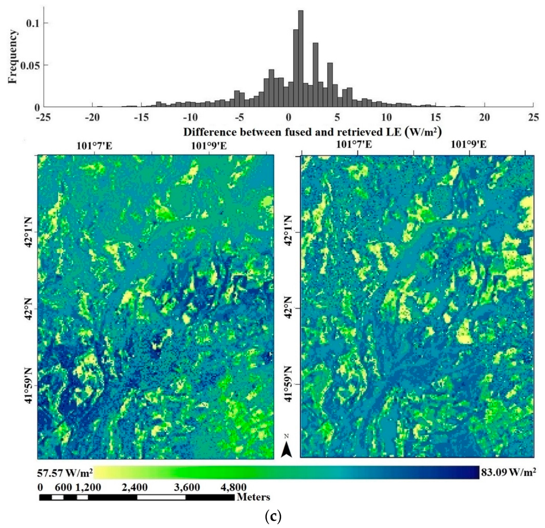
The performance of the SADFAET was first evaluated through the comparison of fused ET data with the retrieved ET data by the ESVEP model using the Landsat 8 data on the 10 selected fusion dates. Three typical pairs of the spatial pattern of fused ET and retrieved ET data over the study area on May 15, July 18 and August 28, together with a histogram of the ET difference, are illustrated in Figure 4. Table 6 illustrates the statistical measures of ET fused by the SADFAET and that retrieved using the Landsat 8 data over the typical days. It could be found that over the study area, the fused ET data were close to the retrieved ET data, with a smaller absolute value of the percent difference varying between 1.0% and 5.6%. The fused ET data also had a standard deviation (SD) magnitude similar to that of compared to the retrieved ET on each of the three typical days. The SD value over the study area varied between 16.2 W/m2 and 48.2 W/m2 for the fused ET and between 17.6 W/m2 and 48.8 W/m2 for the retrieved ET. The mean values over the study area varied between 30.1 W/m2 and 74.6 W/m2 for the fused ET and between 28.5 W/m2 and 76.7 W/m2 for the retrieved ET.
It is clear that the image fused by the SADFAET was similar to that predicted directly using the Landsat 8 image in terms of the overall spatial patterns of ET. The difference between SADFAET ET and Landsat 8 ET is mostly ±10 W/m2. The fused ET images contained most of the spatial details found in the Landsat 8 ET images, including surface features, such as buildings, barren lands (with low ET values) and croplands (with high values).
4.3. Validation of ET Data Fused by the SADFAET Model Using Ground-Based Measurements
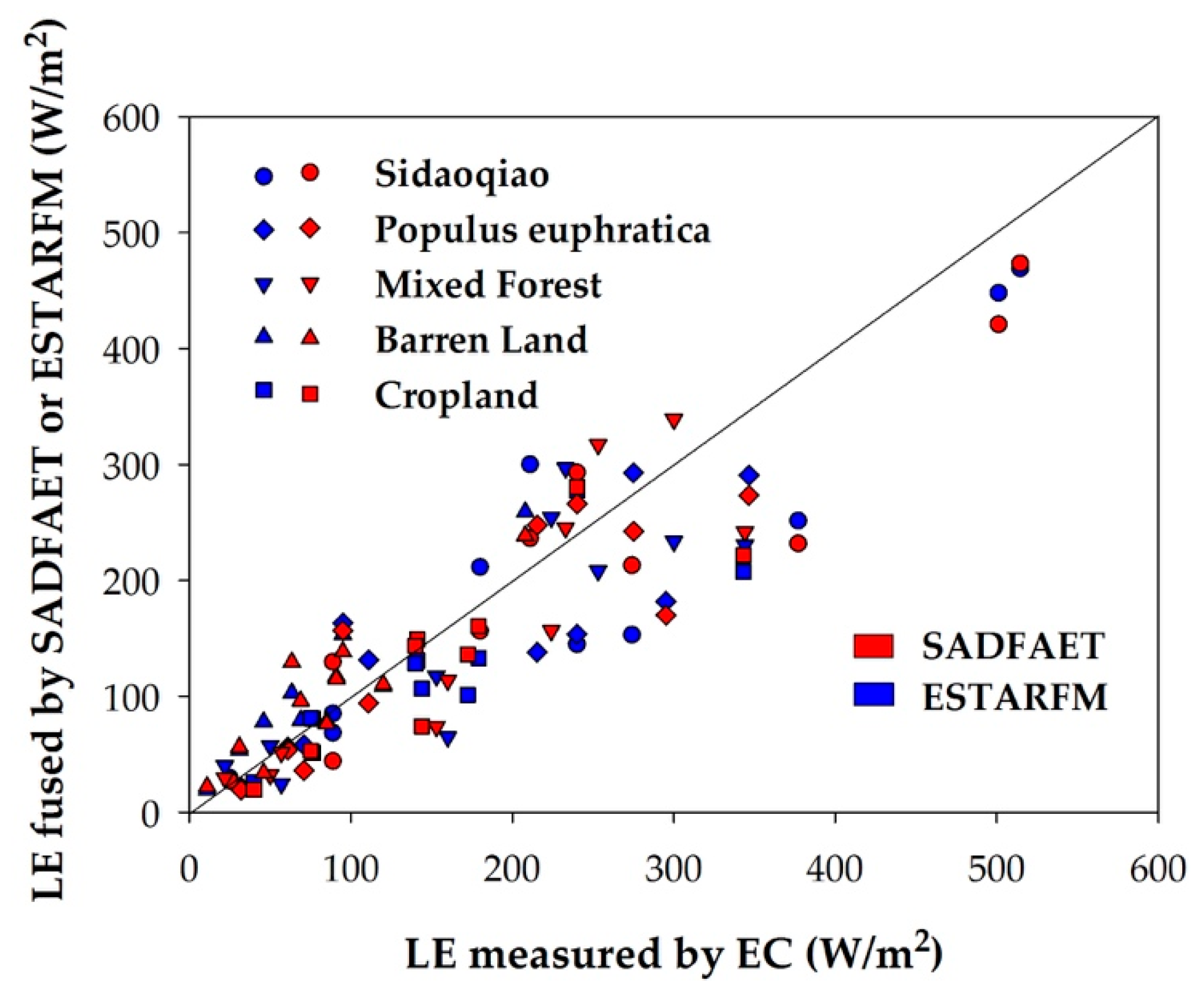
The instantaneous LE data fused by the SADFAET were further compared with the ground-based EC measurement collected at the 5 test sites over the 10 selected days (see Figure 5). Table 7 illustrates the statistical parameters between the fused LEs and measured LEs on the selected days for different land cover types. The results show an overall reasonably good agreement between the instantaneously fused LEs and measured LEs, with a slight underestimation of 13.1 W/m2 and a RMSE of 45.7 W/m2. An overestimation of 18.0 W/m2 was found at the Barren Land site, with a RMSE of 25.1 W/m2, while underestimations were shown at the other four sites, with mean errors varying from −27.5 W/m2 to −18.3 W/m2 and RMSE varying from 41.4 W/m2 to 60.6 W/m2. The verification results at the site scale show that the SADFAET can accurately fuse ET data over most surfaces, while the relatively larger error at the Barren Land site was possibly due to the poor accuracy of the instantaneously retrieved LE.
4.4. Comparison of ET Data Fused by the SADFAET and ESTARFM
We compared the SADFAET with the original ESTARFM to verify the improvement in the SADFAET. The scatter plots in Figure 5 also show the measured LE and ESTARFM LE at the 5 sites. According to Figure 5, we can see that both the SADFAET and ESTARFM can accurately predict ET at a high resolution, while the SADFAET LE data in the scatter plots fall closer to the 1:1 line. For all the sites, the prediction precision of the SADFAET is higher than that of the original ESTARFM (MPE: −5% vs. −8%; MB: −13.1 W/m2 vs. −18.6 W/m2; RMSE: 45.7 W/m2 vs. 50.6 W/m2). Statistics are provided in Figure 6 for different sites for the ESTARFM and SADFAET. Similar to the SADFAET, only fused ET data by the ESTARFM at the Barren Land site were overestimated, while fused ET data at the other sites were underestimated. The greatest improvement in the SADFAET, in comparison to the ESTARFM, appeared at the Cropland site (MPE: −12% vs. −17%), while at the Barren Land site, there was almost no improvement (MPE: 22% vs. 22%). This may be because the SADFAET considers the variation in soil moisture, while the soil moisture of the Bareland site has a low value and the soil moisture of the Cropland site has significant variation during the crop growth season.
4.5. Discussion
4.5.1. Uncertainties in the SADFAET
Our results indicate that the SADFAET can accurately estimate ET at a high spatio-temporal resolution by fusing ET at a high spatial resolution with that at a high temporal resolution. However, there are some uncertainties are associated with the use of the algorithm and the uncertainty in the fused ET method primarily results from (1) the retrieval of surface ET-indicative variables, (2) the fine- and coarse-resolution ET data at the reference and prediction times and (3) the fusion algorithm itself, including the selection of similar neighbouring pixels, the calculation of the weights of these pixels and the determination of the conversion coefficient and the temporal weight. For example, the uncertainties in the remotely sensed and meteorological data could affect the calculation of instantaneous ET from the ESVEP model. Validation results indicated that LE was underestimated at the Sidaoqiao site (16%), Mixed Forest site (3%), Populus euphratica site (12%) and Cropland site (14%), while LE was overestimated at the Barren Land site (22%). The uncertainty in the calculation of the critical surface temperature could cause the inaccurate classification of similar pixels and the computation of the weight of the similar pixel. In addition, the inherent uncertainties in the EC and LAS validation data and the mismatch in the spatial scales between the predicted and fused ET and EC measurements could also impact the fusion accuracy.
4.5.2. Improvements and Limitations of the SADFAET
The SADFAET has made several improvements to the original ESTARFM when it is used for ET fusion. The most significant improvement is the introduction of the critical surface temperature (T*) to consider the impact of soil moisture for the selection of similar pixels, which can solve the problem that determining the number of classes limits automated processing and reduces the accuracy of similar pixel selection in the ESTARFM. In the original ESTARFM, shortwave bands are used to select similar pixels by setting a threshold and unsupervised classification without considering the soil moisture. However, our SADFAET introduced T* to calculate the soil moisture variation between the predicted time (tp) and reference times (tm and tn) of different pixels, which can ensure that the correct similar pixels with similar ET variations are selected. Second, for the weight calculation of each similar pixel, the SADFAET introduces surface ET-indicative similarity to consider the influences of NDVI, LST, soil moisture and ET at tm and tn. Finally, ET may change rapidly with time and using more bands will contribute to accurately computing the weight of the similar pixel; thus, we introduced the shortwave bands (representing vegetation cover), shortwave infrared bands (representing soil moisture) and thermal infrared bands (representing LST) between each similar pixel and its corresponding coarse-resolution pixel for the calculation of spectral similarity. The ET fusion estimates in the present study yielded an MPE of −11% to 22%, which was slightly better than that from previous studies. For example, Ma et al. [28] reported MPE values of −14% to 29% in the midstream region of the Heihe River basin when the ESTARFM was used to fuse ET retrieved from Landsat 7 ETM+ and MODIS data. Semmens et al. [13] and Yang et al. [16] employed the original STARFM combined with a multi-scale ET retrieval algorithm to compute 30 m resolution ET over a mixed forested/agricultural landscape in North Carolina, USA and the mean absolute percent errors of the fused ET were 20% to 23% and 19% to 30% respectively. For the same study area, the prediction precision of the SADFAET is higher than that of the original ESTARFM (−14% to 22%) and the fused ET images contained most of the spatial details found in the Landsat 8 ET images.
There are several limitations and constraints when using the SADFAET. First, similar to the ESTARFM and STARFM [35,36], the SADFAET cannot accurately predict shape changes and may cause boundary blurring. Second, when the soil moisture maintains a low value or exhibits slight variation, the accuracy of the SADFAET may decrease. Finally, although the SADFAET solves the problem whereby determining the number of classes limits automated processing in the ESTARFM, the size of the moving window remains a restriction.
5. Conclusions
This research proposed a spatio-temporal adaptive data fusion algorithm for evapotranspiration mapping (SADFAET) to estimate evapotranspiration (ET) at high spatial resolutions (30 m) and at a high temporal frequency (daily). An experiment that predicted ET at a 30 m spatial resolution on 10 dates in 2015 from April to October downstream of the Heihe River basin was performed using Landsat 8 and MODIS datasets. The main advantage of SADFAET is the consideration of soil moisture by introducing the critical surface temperature (T*) during the selection of similar pixels. The other improvement is the use of multiple spectral bands, including shortwave bands (representing vegetation cover), shortwave infrared bands (representing soil moisture) and thermal infrared bands (representing LST) and the introduction of the surface ET-indicative similarity to calculate the weights of similar pixels.
The results showed an overall reasonably good agreement between the fused ET and measured ET with a slight underestimation of 13.1 W/m2 and a RMSE of 45.7 W/ m2. The difference between SADFAET ET and Landsat 8 ET was mostly ±10 W/m2 and the SADFAET ET images preserved most of the original spatial details. The prediction precision of the SADFAET was higher than that of the original ESTARFM (MPE: −5% vs. −8%; MB: −13.1 W/m2 vs. −18.6 W/m2; RMSE: 45.7 W/m2 vs. 50.6 W/m2). Therefore, our proposed SADFAET could effectively fuse ET at high and low spatial resolutions and the method was better than that from previous studies and other common fusion algorithms. Future work will be performed on the evaluation of the SADFAET on other regions that are covered by different vegetation types and characterized by different climates.
Author Contributions
R.T. and T.W. designed the experiments; T.W. and R.T. analyzed the data and wrote the paper; Z.L, Y.J., M.L. and L.N. revised the paper.
Funding
This research was funded by the National Key R&D Program of China under Grant 2018YFA0605401, the Beijing Municipal Science and Technology Project under Grant Z181100005318003, the Youth Innovation Promotion Association CAS under 2015039, the National Natural Science Foundation of China under Grant 41571351 and 41571367.
Acknowledgments
The staff members in the Heihe Watershed Allied Telemetry Experimental Research (HiWATER) experimental areas are acknowledged for their hard work on the setup and maintenance of the ground-based instruments and data collection.
Conflicts of Interest
The authors declare no conflict of interest.
References
- Li, A.; Zhao, W.; Deng, W. A Quantitative Inspection on Spatio-Temporal Variation of Remote Sensing-Based Estimates of Land Surface Evapotranspiration in South Asia. Remote Sens. 2015, 7, 4726–4752. [Google Scholar] [CrossRef] [Green Version]
- Mahour, M.; Tolpekin, V.; Stein, A.; Sharifi, A. A comparison of two downscaling procedures to increase the spatial resolution of mapping actual evapotranspiration. ISPRS J. Photogramm. Remote Sens. 2017, 126, 56–67. [Google Scholar] [CrossRef]
- Weng, Q.; Fu, P.; Gao, F. Generating daily land surface temperature at Landsat resolution by fusing Landsat and MODIS data. Remote Sens. Environ. 2014, 145, 55–67. [Google Scholar] [CrossRef]
- Guo, L.J.; Moore, J.M. Pixel block intensity modulation: Adding spatial detail to TM band 6 thermal imagery. Int. J. Remote Sens. 1998, 19, 2477–2491. [Google Scholar] [CrossRef]
- Nichol, J. An emissivity modulation method for spatial enhancement of thermal satellite images in urban heat island analysis. Photogramm. Eng. Remote Sens. 2009, 75, 547–556. [Google Scholar] [CrossRef]
- Hong, S.-H.; Hendrickx, J.M.H.; Borchers, B. Down-scaling of SEBAL derived evapotranspiration maps from MODIS (250 m) to Landsat (30 m) scales. Int. J. Remote Sens. 2011, 32, 6457–6477. [Google Scholar] [CrossRef]
- Anderson, M.C.; Kustas, W.P.; Norman, J.M.; Hain, C.R. Mapping daily evapotranspiration at field to global scales using geostationary and polar orbiting satellite imagery. Hydrol. Earth Syst. Sci. 2011, 15, 223–239. [Google Scholar] [CrossRef]
- Anderson, M.C.; Kustas, W.P.; Alfieri, J.G.; Gao, F.; Hain, C.; Prueger, J.H.; Evett, S.; Colaizzi, P.; Howell, T.; Chávez, J.L. Mapping daily evapotranspiration at Landsat spatial scales during the BEAREX’08 field campaign. Adv. Water Resour. 2012, 50, 162–177. [Google Scholar] [CrossRef]
- Anderson, M.C.; Allen, R.G.; Morse, A.; Kustas, W.P. Use of Landsat thermal imagery in monitoring evapotranspiration and managing water resources. Remote Sens. Environ. 2012, 122, 50–65. [Google Scholar] [CrossRef]
- Cammalleri, C.; Anderson, M.C.; Gao, F.; Hain, C.R.; Kustas, W.P. A data fusion approach for mapping daily evapotranspiration at field scale. Water Resour. Res. 2013, 49, 4672–4686. [Google Scholar] [CrossRef] [Green Version]
- Cammalleri, C.; Anderson, M.C.; Gao, F.; Hain, C.R.; Kustas, W.P. Mapping daily evapotranspiration at field scales over rainfed and irrigated agricultural areas using remote sensing data fusion. Agric. For. Meteorol. 2014, 186, 1–11. [Google Scholar] [CrossRef] [Green Version]
- Bhattarai, N.; Quackenbush, L.J.; Dougherty, M.; Marzen, L.J. A simple Landsat–MODIS fusion approach for monitoring seasonal evapotranspiration at 30 m spatial resolution. Int. J. Remote Sens. 2015, 36, 115–143. [Google Scholar]
- Semmens, K.A.; Anderson, M.C.; Kustas, W.P.; Gao, F.; Alfieri, J.G.; Mckee, L.; Prueger, J.H.; Hain, C.R.; Cammalleri, C.; Yang, Y.; et al. Monitoring daily evapotranspiration over two California vineyards using Landsat 8 in a multi-sensor data fusion approach. Remote Sens. Environ. 2015, 185, 155–170. [Google Scholar] [CrossRef]
- Ke, Y.; Im, J.; Park, S.; Gong, H. Downscaling of MODIS One Kilometer Evapotranspiration Using Landsat-8 Data and Machine Learning Approaches. Remote Sens. 2016, 8, 215. [Google Scholar] [CrossRef]
- Bastiaanssen, W.; Noordman, E.; Pelgrum, H.; Davids, G.; Thoreson, B.; Allen, R. SEBAL model with remotely sensed data to improve water-resources management under actual field conditions. J. Irrig. Drain. Eng. 2005, 131, 85–93. [Google Scholar] [CrossRef]
- Allen, R.G.; Robison, C.W.; Trezza, R.; Garcia, M.; Kjaersgaard, J. Comparison of evapotranspiration images from MODIS and Landsat along the Middle Rio Grande of New Mexico. In Proceedings of the 17th William T. Pecora Memorial Remote Sensing Symposium Proceedings, Denver, CO, USA, 18–20 November 2008. [Google Scholar]
- Yang, Y.; Shang, S.; Jiang, L. Remote sensing temporal and spatial patterns of evapotranspiration and the responses to water management in a large irrigation district of North China. Agric. For. Meteorol. 2012, 164, 112–122. [Google Scholar] [CrossRef]
- Yang, Y.; Anderson, M.C.; Gao, F.; Hain, C.R.; Semmens, K.A.; Kustas, W.P.; Noormets, A.; Wynne, R.H.; Thomas, V.A.; Sun, G. Daily Landsat-scale evapotranspiration estimation over a forested landscape in North Carolina, USA, using multi-satellite data fusion. Hydrol. Earth Syst. Sci. 2017, 21, 1017–1037. [Google Scholar] [CrossRef] [Green Version]
- Wu, P.; Shen, H.; Zhang, L.; Göttsche, F.M. Integrated fusion of multi-scale polar-orbiting and geostationary satellite observations for the mapping of high spatial and temporal resolution land surface temperature. Remote Sens. Environ. 2015, 156, 169–181. [Google Scholar] [CrossRef]
- Zayed, I.S.A.; Elagib, N.A.; Ribbe, L.; Heinrich, J. Satellite-based evapotranspiration over Gezira Irrigation Scheme, Sudan: A comparative study. Agric. Water Manag. 2016, 177, 66–76. [Google Scholar] [CrossRef]
- Allen, R.; Tasumi, M.; Trezza, R.; Kjaersgaard, J. Mapping Evapotranspiration at High Resolution, Applications Manual for Landsat Satellite Imagery; University of Idaho: Kimberly, ID, USA, 2010; Volume 2, p. 248. [Google Scholar]
- Yi, Z.; Zhao, H.; Jiang, Y.; Yan, H.; Yin, C.; Huang, Y.; Zhen, H. Daily Evapotranspiration Estimation at the Field Scale: Using the Modified SEBS Model and HJ-1 Data in a Desert-Oasis Area, Northwestern China. Water 2018, 10, 640. [Google Scholar] [CrossRef]
- Yang, G.; Weng, Q.; Pu, R.; Gao, F.; Sun, C.; Li, H.; Zhao, C. Evaluation of ASTER-Like Daily Land Surface Temperature by Fusing ASTER and MODIS Data during the HiWATER-MUSOEXE. Remote Sens. 2016, 8, 75. [Google Scholar] [CrossRef]
- Bai, Y.; Wong, M.S.; Shi, W.-Z.; Wu, L.-X.; Qin, K. Advancing of Land Surface Temperature Retrieval Using Extreme Learning Machine and Spatio-Temporal Adaptive Data Fusion Algorithm. Remote Sens. 2015, 7, 4424–4441. [Google Scholar] [CrossRef] [Green Version]
- Oliveraguerra, L.; Mattar, C.; Merlin, O.; DuránAlarcón, C.; SantamaríaArtigas, A.; Fuster, R. An operational method for the disaggregation of land surface temperature to estimate actual evapotranspiration in the arid region of Chile. ISPRS J. Photogramm. Remote Sens. 2017, 128, 170–181. [Google Scholar] [CrossRef]
- Ke, Y.; Im, J.; Park, S.; Gong, H. Spatiotemporal downscaling approaches for monitoring 8-day 30 m actual evapotranspiration. ISPRS J. Photogramm. Remote Sens. 2017, 126, 79–93. [Google Scholar] [CrossRef]
- Yan, L.; Huang, C.; Hou, J.; Gu, J.; Zhu, G.; Xin, L. Mapping daily evapotranspiration based on spatiotemporal fusion of ASTER and MODIS images over irrigated agricultural areas in the Heihe River Basin, Northwest China. Agric. For. Meteorol. 2017, 244, 82–97. [Google Scholar]
- Ma, Y.; Liu, S.; Song, L.; Xu, Z.; Liu, Y.; Xu, T.; Zhu, Z. Estimation of daily evapotranspiration and irrigation water efficiency at a Landsat-like scale for an arid irrigation area using multi-source remote sensing data. Remote Sens. Environ. 2018, 216, 715–734. [Google Scholar] [CrossRef]
- Najmaddin, P.M.; Whelan, M.J.; Balzter, H. Estimating Daily Reference Evapotranspiration in a Semi-Arid Region Using Remote Sensing Data. Remote Sens. 2017, 9, 779. [Google Scholar] [CrossRef]
- Stefan, V.; Merlin, O.; Er-Raki, S.; Escorihuela, M.-J.; Khabba, S. Consistency between in situ, model-derived and high-resolution-image-based soil temperature endmembers: Towards a robust data-based model for multi-resolution monitoring of crop evapotranspiration. Remote Sens. 2015, 7, 10444–10479. [Google Scholar] [CrossRef]
- Kuriqi, A. Assessment and quantification of meteorological data for implementation of weather radar in mountainous regions. MAUSAM 2016, 67, 789–802. [Google Scholar]
- Martínez-de la Torre, A.; Blyth, E.M.; Robinson, E.L. Evaluation of drydown processes in global land surface and hydrological models using flux tower evapotranspiration. Water 2019, 11, 356. [Google Scholar] [CrossRef]
- Small, E.; Badger, A.; Abolafia-Rosenzweig, R.; Livneh, B. Estimating Soil Evaporation Using Drying Rates Determined from Satellite-Based Soil Moisture Records. Remote Sens. 2018, 10, 1945. [Google Scholar] [CrossRef]
- Bruin, H.A.; Trigo, I.F. A New Method to Estimate Reference Crop Evapotranspiration from Geostationary Satellite Imagery: Practical Considerations. Water 2019, 11, 382. [Google Scholar] [CrossRef]
- Zhu, X.L.; Jin, C.; Feng, G.; Chen, X.H.; Masek, J.G. An enhanced spatial and temporal adaptive reflectance fusion model for complex heterogeneous regions. Remote Sens. Environ. 2010, 114, 2610–2623. [Google Scholar] [CrossRef]
- Gao, F.; Masek, J.; Schwaller, M.; Hall, F. On the blending of the Landsat and MODIS surface reflectance: Predicting daily Landsat surface reflectance. IEEE Trans. Geosci. Remote Sens. 2006, 44, 2207–2218. [Google Scholar]
- Emelyanova, I.V.; Mcvicar, T.R.; Niel, T.G.V.; Li, L.T.; van Dijk, A.I. Assessing the accuracy of blending Landsat–MODIS surface reflectances in two landscapes with contrasting spatial and temporal dynamics: A framework for algorithm selection. Remote Sens. Environ. 2013, 133, 193–209. [Google Scholar] [CrossRef]
- Bai, L.; Cai, J.; Liu, Y.; Chen, H.; Zhang, B.; Huang, L. Responses of field evapotranspiration to the changes of cropping pattern and groundwater depth in large irrigation district of Yellow River basin. Agric. Water Manag. 2017, 188, 1–11. [Google Scholar] [CrossRef]
- Tang, R.; Li, Z.L. An End-Member-Based Two-Source Approach for Estimating Land Surface Evapotranspiration From Remote Sensing Data. IEEE Trans. Geosci. Remote Sens. 2017, 55, 5818–5832. [Google Scholar] [CrossRef]
- Vicente-Serrano, S.M.; Cabello, D.; Tomás-Burguera, M.; Martín-Hernández, N.; Beguería, S.; Azorin-Molina, C.; Kenawy, A.E. Drought Variability and Land Degradation in Semiarid Regions: Assessment Using Remote Sensing Data and Drought Indices (1982–2011). Remote Sens. 2015, 7, 4391–4423. [Google Scholar] [CrossRef] [Green Version]
- Fensholt, R.; Sandholt, I. Derivation of a shortwave infrared water stress index from MODIS near-and shortwave infrared data in a semiarid environment. Remote Sens. Environ. 2003, 87, 111–121. [Google Scholar] [CrossRef]
- Ghulam, A.; Li, Z.-L.; Qin, Q.; Tong, Q.; Wang, J.; Kasimu, A.; Zhu, L. A method for canopy water content estimation for highly vegetated surfaces-shortwave infrared perpendicular water stress index. Sci. China Ser. D Earth Sci. 2007, 50, 1359–1368. [Google Scholar] [CrossRef]
- Zhang, N.; Hong, Y.; Qin, Q.; Liu, L. VSDI: A visible and shortwave infrared drought index for monitoring soil and vegetation moisture based on optical remote sensing. Int. J. Remote Sens. 2013, 34, 4585–4609. [Google Scholar] [CrossRef]
- Talsma, C.; Good, S.; Miralles, D.; Fisher, J.; Martens, B.; Jimenez, C.; Purdy, A. Sensitivity of Evapotranspiration Components in Remote Sensing-Based Models. Remote Sens. 2018, 10, 1601. [Google Scholar] [CrossRef]
- Campo-Bescós, M.A.; Muñoz-Carpena, R.; Southworth, J.; Zhu, L.; Waylen, P.R.; Bunting, E. Combined Spatial and Temporal Effects of Environmental Controls on Long-Term Monthly NDVI in the Southern Africa Savanna. Remote Sens. 2013, 5, 6513–6538. [Google Scholar] [CrossRef] [Green Version]
- Kustas, W.P.; Norman, J.M. A two-source energy balance approach using directional radiometric temperature observations for sparse canopy covered surfaces. Agron. J. 2000, 92, 847–854. [Google Scholar] [CrossRef]
- Liu, S.M.; Xu, Z.W.; Wang, W.; Jia, Z.; Zhu, M.; Bai, J.; Wang, J. A comparison of eddy-covariance and large aperture scintillometer measurements with respect to the energy balance closure problem. Hydrol. Earth Syst. Sci. 2011, 15, 1291–1306. [Google Scholar] [CrossRef] [Green Version]
- Liu, S.; Li, X.; Xu, Z.; Che, T.; Xiao, Q.; Ma, M.; Liu, Q.; Jin, R.; Guo, J.; Wang, L.; et al. The Heihe Integrated Observatory Network: A basin-scale land surface processes observatory in China. Vadose Zone J. 2018, 17. [Google Scholar] [CrossRef]
- Li, X.; Cheng, G.; Liu, S.; Xiao, Q.; Ma, M.; Jin, R.; Che, T.; Liu, Q.; Wang, W.; Qi, Y. Heihe Watershed Allied Telemetry Experimental Research (HiWATER): Scientific Objectives and Experimental Design. Bull. Am. Meteorol. Soc. 2013, 94, 1145–1160. [Google Scholar] [CrossRef]
- Sadeghi, M.; Babaeian, E.; Tuller, M.; Jones, S.B. The optical trapezoid model: A novel approach to remote sensing of soil moisture applied to Sentinel-2 and Landsat-8 observations. Remote Sens. Environ. 2017, 198, 52–68. [Google Scholar] [CrossRef] [Green Version]
- Qin, Z.; Karnieli, A.; Berliner, P. A mono-window algorithm for retrieving land surface temperature from Landsat TM data and its application to the Israel-Egypt border region. Int. J. Remote Sens. 2001, 22, 3719–3746. [Google Scholar] [CrossRef]
- Sobrino, J.A.; Jimenez-Muoz, J.C.; Sòria, G.; Romaguera, M.; Guanter, L.; Moreno, J.; Plaza, A.; Martínez, P. Land surface emissivity retrieval from different VNIR and TIR sensors. IEEE Trans. Geosci. Remote Sens. 2008, 46, 316–327. [Google Scholar] [CrossRef]
Figure 1.
Schematic diagram of the spatio-temporal adaptive data fusion algorithm for evapotranspiration mapping (SADFAET).
Figure 1.
Schematic diagram of the spatio-temporal adaptive data fusion algorithm for evapotranspiration mapping (SADFAET).

Figure 2.
The location of the test area over the Heihe Watershed Allied Telemetry Experimental Research (HiWATER) experimental areas [49].
Figure 2.
The location of the test area over the Heihe Watershed Allied Telemetry Experimental Research (HiWATER) experimental areas [49].

Figure 3.
Validation of the instantaneous LE estimations from the end-member-based soil and vegetation energy partitioning (ESVEP) model for MODIS- and Landsat-based retrievals against ground-based LAS (red symbols) and EC (blue symbols) measurements.
Figure 3.
Validation of the instantaneous LE estimations from the end-member-based soil and vegetation energy partitioning (ESVEP) model for MODIS- and Landsat-based retrievals against ground-based LAS (red symbols) and EC (blue symbols) measurements.

Figure 4.
Histogram (top panel) of the difference between fine-resolution LE data fused by the SADFAET (right panel) and the estimates directly retrieved by the ESVEP model using Landsat 8 data (left panel) on (a) May 15, (b) July 18 and (c) August 28.
Figure 4.
Histogram (top panel) of the difference between fine-resolution LE data fused by the SADFAET (right panel) and the estimates directly retrieved by the ESVEP model using Landsat 8 data (left panel) on (a) May 15, (b) July 18 and (c) August 28.


Figure 5.
Comparison of instantaneous LE predictions using the SADFAET and ESTARFM with LE measured by EC.
Figure 5.
Comparison of instantaneous LE predictions using the SADFAET and ESTARFM with LE measured by EC.

Figure 6.
Statistical parameters between the instantaneous LE predictions using ESTARFM/ SADFAET and the EC values: (a) RMSE; (b) MB; (c) MPE.
Figure 6.
Statistical parameters between the instantaneous LE predictions using ESTARFM/ SADFAET and the EC values: (a) RMSE; (b) MB; (c) MPE.


Table 1.
Attributes of the test sites in the study area (Sidaoqiao).
| Ground Sites | Landscape | Longitude | Latitude | Elevation (m) | Observation Instrument |
|---|---|---|---|---|---|
| Sidaoqiao | tamarix | 101.1374 E | 42.0012 N | 873 | LAS/EC |
| Populus euphratica | populus euphratica | 101.1239 E | 41.9932 N | 876 | EC |
| Mixed Forest | populus euphratica and tamarix | 101.1335 E | 41.9903 N | 874 | EC |
| Barren Land | bare land | 101.1326 E | 41.9993 N | 878 | EC |
| Cropland | melon | 101.1338 E | 42.0048 N | 875 | EC |
Table 2.
Terra, Moderate Resolution Imaging Spectroradiometer (MODIS) and Landsat 8 data (April to October 2015) used in this study.
Table 2.
Terra, Moderate Resolution Imaging Spectroradiometer (MODIS) and Landsat 8 data (April to October 2015) used in this study.
| Data Type | MODIS (Horizontal 25, Vertical 04) | Landsat 8 (Path 133/134, Row 031) | ||
|---|---|---|---|---|
| MOD09GA | MOD021KM etc. | OLI | TIRS | |
| Resolution | 500 m | 1000 m | 30 m | 30 m (resample) |
| Day of year (DOY) | 096–304 | 096, 103, 135, 144, 160, 176, 199, 215, 231, 240, 247, 256, 288, 295, 304, | ||
Table 3.
Fusion strategy: day of year (DOY) of the input data and results.
| DOY of MODIS ET (1 km) | DOY of Landsat 8 ET (30 m) | DOY of Fusion Results and Validation (30 m) |
|---|---|---|
| 96/103/135 | 96/135 | 103 |
| 103/135/144 | 103/144 | 135 |
| 135/144/176 | 135/176 | 144 |
| 144/176/199 | 144/199 | 176 |
| 176/199/231 | 176/231 | 199 |
| 199/231/240 | 199/240 | 231 |
| 231/240/247 | 231/247 | 240 |
| 240/247/256 | 240/256 | 247 |
| 247/256/288 | 247/288 | 256 |
| 256/288/295 | 256/295 | 288 |
Table 4.
Summary of the primary inputs into the SADFAET (Landsat and MODIS).
| Variable | MODIS | Landsat 8 |
|---|---|---|
| NDVI | MOD13A2 | OLI Band 4, Band 5 |
| LST | MOD11A1 | TIRS Band 10, mono-window algorithm [51] |
| SM | - | OLI Band 7, OPTRAM [50] |
Table 5.
Error metrics of instantaneous LE estimates from MODIS and Landsat 8 data. Mean O: mean observation; Mean P: mean prediction; MB: mean bias; MPE: mean percent error; RMSE: root mean square error.
Table 5.
Error metrics of instantaneous LE estimates from MODIS and Landsat 8 data. Mean O: mean observation; Mean P: mean prediction; MB: mean bias; MPE: mean percent error; RMSE: root mean square error.
| Ground Sites | Mean O (W/m2) | Mean P (W/m2) | MB (W/m2) | MPE (%) | RMSE (W/m2) |
|---|---|---|---|---|---|
| Sidaoqiao | 217.5 | 189.7 | −27.8 | −16 | 42.7 |
| Populus euphratica | 160.7 | 144.7 | −16.0 | −12 | 40.4 |
| Mixed Forest | 155.4 | 154.2 | −1.2 | −3 | 44.8 |
| Barren Land | 70.5 | 86.7 | 16.2 | 22 | 24.6 |
| Cropland | 135.1 | 120.3 | −14.8 | −14 | 31.8 |
| Average | 147.8 | 139.1 | −8.7 | −5 | 40.9 |
Table 6.
Comparison between instantaneous ET fused by the SADFAET and that directly retrieved by the ESVEP model from Landsat 8 data on typical days (in spring, summer and autumn) over the study area. Max: maximum ET; Min: minimum ET; SD: standard deviation; R: correlation coefficient.
Table 6.
Comparison between instantaneous ET fused by the SADFAET and that directly retrieved by the ESVEP model from Landsat 8 data on typical days (in spring, summer and autumn) over the study area. Max: maximum ET; Min: minimum ET; SD: standard deviation; R: correlation coefficient.
| DOY | Item | Mean (W/m2) | Max (W/m2) | Min (W/m2) | SD (W/m2) | R |
|---|---|---|---|---|---|---|
| May 15 | Fused ET | 30.06 | 45.09 | 10.49 | 16.17 | 0.47 |
| Retrieved ET | 28.48 | 40.84 | 12.76 | 17.58 | ||
| July 18 | Fused ET | 74.61 | 99.26 | 38.29 | 38.85 | 0.49 |
| Retrieved ET | 76.69 | 108.05 | 34.32 | 40.55 | ||
| August 28 | Fused ET | 69.58 | 67.21 | 32.61 | 48.21 | 0.46 |
| Retrieved ET | 68.90 | 83.09 | 29.21 | 48.78 |
Table 7.
Error metrics of the LE fused by the SADFAET with the ground-based EC measurement.
| Ground Sites | Mean O (W/m2) | MB (W/m2) | MPE (%) | RMSE (W/m2) |
|---|---|---|---|---|
| Sidaoqiao | 250.0 | −27.5 | −11 | 60.6 |
| Populus euphratica | 174.2 | −18.3 | −11 | 50.7 |
| Mixed Forest | 179.6 | −19.5 | −11 | 50.5 |
| Barren Land | 81.9 | 18.0 | 22 | 25.1 |
| Cropland | 155.1 | −18.6 | −12 | 41.4 |
| Average | 168.2 | −13.1 | −5 | 45.7 |
© 2019 by the authors. Licensee MDPI, Basel, Switzerland. This article is an open access article distributed under the terms and conditions of the Creative Commons Attribution (CC BY) license (http://creativecommons.org/licenses/by/4.0/).
Share and Cite
MDPI and ACS Style
Wang, T.; Tang, R.; Li, Z.-L.; Jiang, Y.; Liu, M.; Niu, L. An Improved Spatio-Temporal Adaptive Data Fusion Algorithm for Evapotranspiration Mapping. Remote Sens. 2019, 11, 761. https://doi.org/10.3390/rs11070761
AMA Style
Wang T, Tang R, Li Z-L, Jiang Y, Liu M, Niu L. An Improved Spatio-Temporal Adaptive Data Fusion Algorithm for Evapotranspiration Mapping. Remote Sensing. 2019; 11(7):761. https://doi.org/10.3390/rs11070761
Chicago/Turabian StyleWang, Tong, Ronglin Tang, Zhao-Liang Li, Yazhen Jiang, Meng Liu, and Lu Niu. 2019. "An Improved Spatio-Temporal Adaptive Data Fusion Algorithm for Evapotranspiration Mapping" Remote Sensing 11, no. 7: 761. https://doi.org/10.3390/rs11070761
Note that from the first issue of 2016, this journal uses article numbers instead of page numbers. See further details here.