
Accuracy Improvements to Pixel-Based and Object-Based LULC Classification with Auxiliary Datasets from Google Earth Engine


1
School of Geography and Ocean Science, Nanjing University, Nanjing 210023, China
2
School of Geography and Tourism, Anhui Normal University, Wuhu 241002, China
3
Jiangsu Provincial Key Laboratory of Geographic Information Science and Technology, Nanjing University, Nanjing 210023, China
*
Author to whom correspondence should be addressed.
Remote Sens. 2021, 13(3), 453; https://doi.org/10.3390/rs13030453
Submission received: 22 December 2020
/
Revised: 19 January 2021
/
Accepted: 22 January 2021
/
Published: 28 January 2021
(This article belongs to the Collection Google Earth Engine Applications)
Abstract
:The monitoring and assessment of land use/land cover (LULC) change over large areas are significantly important in numerous research areas, such as natural resource protection, sustainable development, and climate change. However, accurately extracting LULC only using the spectral features of satellite images is difficult owing to landscape heterogeneities over large areas. To improve the accuracy of LULC classification, numerous studies have introduced other auxiliary features to the classification model. The Google Earth Engine (GEE) not only provides powerful computing capabilities, but also provides a large amount of remote sensing data and various auxiliary datasets. However, the different effects of various auxiliary datasets in the GEE on the improvement of the LULC classification accuracy need to be elucidated along with methods that can optimize combinations of auxiliary datasets for pixel- and object-based classification. Herein, we comprehensively analyze the performance of different auxiliary features in improving the accuracy of pixel- and object-based LULC classification models with medium resolution. We select the Yangtze River Delta in China as the study area and Landsat-8 OLI data as the main dataset. Six types of features, including spectral features, remote sensing multi-indices, topographic features, soil features, distance to the water source, and phenological features, are derived from auxiliary open-source datasets in GEE. We then examine the effect of auxiliary datasets on the improvement of the accuracy of seven pixels-based and seven object-based random forest classification models. The results show that regardless of the types of auxiliary features, the overall accuracy of the classification can be improved. The results further show that the object-based classification achieves higher overall accuracy compared to that obtained by the pixel-based classification. The best overall accuracy from the pixel-based (object-based) classification model is 94.20% (96.01%). The topographic features play the most important role in improving the overall accuracy of classification in the pixel- and object-based models comprising all features. Although a higher accuracy is achieved when the object-based method is used with only spectral data, small objects on the ground cannot be monitored. However, combined with many types of auxiliary features, the object-based method can identify small objects while also achieving greater accuracy. Thus, when applying object-based classification models to mid-resolution remote sensing images, different types of auxiliary features are required. Our research results improve the accuracy of LULC classification in the Yangtze River Delta and further provide a benchmark for other regions with large landscape heterogeneity.
1. Introduction
Detailed land use/land cover (LULC) information at global and regional scales is essential in many applications, such as natural resource protection, sustainable development, and climate change [1,2,3]. Remote sensing data are widely used to obtain LULC information [4]. However, for large areas with spatial heterogeneity, achieving high accuracy in LULC classifications with only satellite data is difficult [5]. With the availability of other auxiliary datasets, researchers have attempted to improve the accuracy of LULC classification by combining satellite data and auxiliary datasets [6].
The importance of combining auxiliary features (also known as auxiliary data or multi-source data) with remote sensing data to improve the classification accuracy at both regional and global scales has been a topic of interest for 40 years [7,8]. Studies have focused on the assumption that the distribution of vegetation is directly or indirectly related to natural factors [9,10]. Therefore, topography, soil type, and water source can be used as auxiliary features to explain the distribution of vegetation and improve the accuracy of land use classification [11]. In addition to natural factors, remote sensing indices and time series of remote sensing images are also used as auxiliary features for LULC classification [12]. Due to the complexity of the real ground surface, the accuracy of land-use types with various remote sensing indices is highly different [13]. Therefore, multiple remote sensing indices are often used as auxiliary features to distinguish specific LULC types [14]. A remote sensing time series (RSTS) includes long-term repeated observations of the same area [15]. Such data can effectively explain the changes in spectral characteristics caused by different LULC types, or plant growing cycles (phenological characteristics). Therefore, RSTS can also effectively improve the accuracy of LULC classification [16]. Spectral-temporal metrics, a commonly used RSTS, is often adopted as the main or auxiliary features in LULC classification [17].
Although auxiliary features can improve the accuracy of LULC classification, there are two main reasons that restrict the wider use of open-source spatial datasets [18]. The availability of free and open spatial datasets is limited. These datasets must be requested and obtained from multiple sources. Due to computing and storage limits, only a limited number of features can be used in classification models [11]. Google Earth Engine (GEE) provides a powerful cloud-based platform for planetary-scale geospatial analysis that can directly call multi-petabyte satellite imagery and various types of geospatial datasets [19]. GEE is widely used for high-precision land use classification at regional, national, and even global scales [20].
Much previous research using auxiliary features to improve classification accuracy with medium-resolution satellite imagery has focused on pixel-based classification and less on object-based classification [21,22]. LULC classification can be divided into two types according to the classification objects: pixel- and object-based image analysis (OBIA) [23]. LULC types are often difficult to separate spectrally due to low inter-class separability and high intra-class variability [24]. In such cases, the auxiliary features can improve the accuracy of LULC classification because they can provide information beyond the spectrum [25]. Nevertheless, comparative analysis of the differences and similarities of different auxiliary features to improve the classification accuracy between the pixel- and object-based classification methods call for careful study [26]. To ensure that our experiments can be carried out in the lacking data area, we chose open-source datasets that can be directly used in GEE to calculate the auxiliary features, including remote sensing multi-indices, terrain characteristics, soil characteristics, distance to the water source, and spectral–temporal metrics. We then analyzed the performance of different auxiliary features in both pixel- and object-based LULC classifications.
The objectives of this study are to identify (1) which type of auxiliary features is most useful in pixel- and object-based model and (2) the similarities and differences in the various auxiliary features to improve the classification accuracy of the pixel- and object-based classification methods. To achieve our objectives, we examined the performance of 14 random forest (RF) classification models (seven pixel-based RF models and seven object-based RF models) based on six common types of auxiliary features. Our results provide insights for improving the classification accuracy in areas with strong landscape heterogeneity (similar to the Yangtze River Delta) and advice on selecting the optimal combination of auxiliary features to achieve high-precision LULC mapping.
2. Study Area and Materials
2.1. Study Area
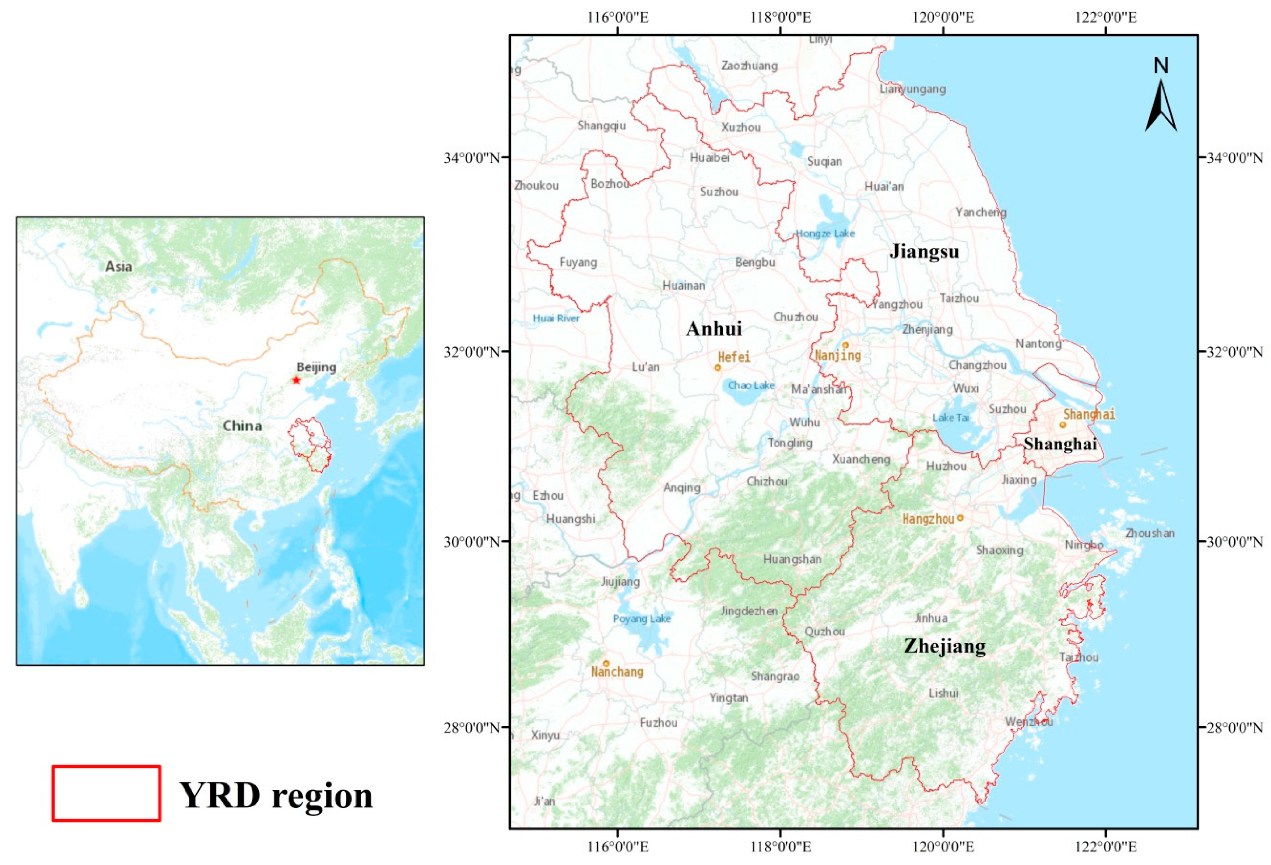
The Yangtze River Delta (YRD) is located along the alluvial plain before the Yangtze River enters the sea. The YRD includes Shanghai city, Jiangsu province, Zhejiang Province, and Anhui Province, with a total area of 348,000 km2 (Figure 1). The YRD has a subtropical monsoon climate, with an average yearly temperature of approximately 14–18 °C, and an average yearly rainfall of approximately 1000–1400 mm [27]. This area is dominated by plains, mainly distributed to the north and east of the YRD. Mountains and hills are mainly distributed to the southwest of the YRD. Affected by topography and climate, the YRD has strong landscape heterogeneity [28].
The YRD is one of China’s most developed economic regions consisting of the YRD urban agglomeration, one of the six largest urban agglomerations in the world, which plays an important role in China’s social and economic development [29]. In 2015, the residential population of the YRD was approximately 140 million, accounting for 11.62% of China’s total population; the Gross Domestic Product (GDP) was 1355.2 billion Chinese Yuan, accounting for 20.02% of the national GDP [30]. With the increase in population and rapid economic growth, the regional LULC is constantly changing, which may lead to regional land degradation, land contamination, loss of biodiversity, and other environmental and ecological issues [31]. Accurate and reliable LULC information is required for land sustainability and environmental management in the YRD. Owing to this situation, we chose the YRD as the research area.
2.2. Data Collection and Pre-Processing
2.2.1. Landsat-8 Operational Land Imager (OLI) Imagery
Landsat data are some of the most widely used data in LULC classification [32]. Here, we adopted 2015 Landsat-8 Operational Land Imager surface reflectance tier 1 (Landsat-8 OLI SR T1) data from the GEE as the primary remote sensing information for classification. The medians of the Red, Green, Blue, Near-infrared (NIR), and Short-wave infrared (SWIR-1 and SWIR-2) spectral bands of the Landsat-8 OLI image (denoted as B2–B7) were considered in the analysis. Some studies have shown that the principal component (PC) of the bands can improve the LULC classification accuracy [33]. Therefore, we used the principal component of bands 2–7 in the analysis (see Table 1 and Table 2). The administrative boundary data of the YRD was downloaded from the ArcGIS online website, with which the portions containing the study area were subdivided from all Landsat images.
The image synthesis and cloud mask methods were applied to generate cloud-free composite images for the study period only during the growing season. The Landsat-8 OLI dataset was processed with the C Function of Mask (CFMASK) model for each pixel [14]. The quality of each pixel for water, clouds, snow, and cloud shadows can be extracted from the “pixel_qa” (pixel quality attributes) band [19]. As the annual average temperature in the YRD is approximately 14–18 °C, the YRD is not characterized by permanent snow or ice cover. Here, we mainly extracted cloud and cloud shadow information (see Supplementary Materials: Data Preprocessing).
2.2.2. LULC Reference Data
High precision reference data and an appropriate classification system are the perquisites for LULC classification [34]. In this study, we combined both imagery observation and field investigation to determine the training and validation samples. The training and validation data used in LULC classification should have an extensive amount of data and be also randomly distributed such that the ratio of the data types represents the actual ratio of each LULC type [16]. We collected land survey data for the entire YRD in 2008 and 2010 at a scale of 1:10,000 (see Table 1). The land survey data included six types of LULC (cropland, woodland, grassland, built-up land, water body, and bare land). As the land survey data was in 2008 and 2010, and our study period was 2015, we generated a training and validation sample set in 2015 (as described in Section 3.1). To construct a training and validation sample set in 2015 for classification, we introduced several sets of well-recognized LULC products in the YRD, including MODIS land cover products (MCD12Q1 2008–2015) [35] and global land cover data (GlobCover 2009) [36]. These LULC products have different LULC types; therefore, we reclassified them to the same LULC standard. Based on the same LULC data types, we generated training and verification points in 2015.
2.2.3. Auxiliary Data
We selected the medium-resolution geospatial datasets available on GEE, which are as close as possible to Landsat-8 OLI. The time coverage of these datasets was used to extract auxiliary features, such as the terrain, soil, and phenology (see Table 1 and Figure 2).
Using the preprocessed Landsat-8 OLI images, we obtained the maximum and median values for ten types of spectral indices (see Table 2). Previous studies have shown that different remote sensing indices are sensitive to different types of LULC. Therefore, there is no general index for all LULC types [37]. Previous research has shown that the Normalized Difference Vegetation Index (NDVI) is sensitive to vegetation characteristics [38], the Normalized Difference Water Index (NDWI) is sensitive to water bodies [39], and the Normalized Difference Built-up Index (NDBI) is sensitive to built-up areas [33]. Although vegetation indices, such as NDVI, have been proposed in previous studies to discriminate LULC types, research on forests has revealed that spectral indices including the near-infrared wavelength, present weaker relationships with LULC than the shortwave infrared wavelength, among others. Therefore, we also included the Normalized Burn Ratio (NBR) and Normalized Difference Moisture Index (NDMI) spectral indices to examine their contributions to LULC classification [40]. The Tasselled Cap component is also widely applied to characterize vegetation conditions. These indices measure the presence and density of green vegetation, total reflectance, soil moisture content, and vegetation density (structure) [41]. Thus, we further added the Tasselled Cap Brightness (TCB), Tasselled Cap Greenness (TCG), Tasselled Cap Wetness (TCW), and Tasselled Cap Angle (TCA) to the LULC classification models.
Topographic features are one of the important factors affecting land cover. Local topography is an indirect gradient that moderates vegetation growth and regional climate conditions, such as soil development, and precipitation and temperature regimes [42]. Topographic features generated from Digital Elevation Models (DEMs) include elevation (affecting the temperature and precipitation level), slope, and aspect (affecting the solar radiation and vegetation growth). To describe the terrain features, we used the 30 m DEM generated from the Shuttle Radar Topography Mission (SRTM). This DEM is a post-processed elevation dataset widely used due to its high accuracy and extensive coverage [43]. The distance to the water source is also an essential factor in the healthy growth of many plants [44]. We used the European Commission’s Joint Research Centre (JRC) yearly water classification history to extract the water bodies in the study area and calculated the Euclidean distances between the pixels and water sources [45].
In addition, the main influencing factors for land cover also include soil features [46]. For example, grassland soils have a significantly higher bulk density than soils in natural woody vegetation, which may help in LULC classifications between grasslands and forests. We used the soil data provided by OpenLandMap to describe the changes in the soil characteristics. This dataset provides the soil bulk density, soil clay content, soil taxonomy great groups, soil organic carbon content, soil PH, soil sand content, soil texture class, soil water content, and other soil characteristics. This dataset contains seven depths (0, 5, 15, 30, 60, 100, and 200 cm) for the standard numerical soil characteristics and soil global predictions of the category distributions. Based on the trapezoidal rule suggested by Hengl et al. [47], we utilized the numerical integration to average the soil features of the topsoil (0–15 cm) and subsoil (15–60 cm).
Spectral–temporal metrics are statistical aggregations of quality-screened reflectance or spectral index time-series observations. These metrics are resilient to data gaps caused by persistent cloud cover or system failures and inconsistent numbers of available satellite images. In calculating the spectral–temporal metrics, we only considered the observation results of the vegetation growth period. This is because the vegetation indices in winter are low and it is difficult to distinguish the LULC types. The identification of the vegetative growth period is important for large-scale areas (such as the YRD). A challenge here is to achieve the purpose of automatic identification by performing percentile analysis on all NDVI values during the study period. Only observations with NDVI values higher than 25% were considered to constitute the vegetative growth period; thus, a feature space with 27 spectral–temporal indicators was generated. The growth periods for different vegetation types are different. Therefore, we selected six months before and after 2015 for a total of 24 months to generate the spectral–temporal metrics (see Supplementary Materials Part 2).
3. Methods
Figure 3 illustrates the overall process of this experiment. First, with the support of multi-source LULC products, following the principles of “stable state” and “consistent classification” [9], the reference data were generated and then divided into independent training and verification samples. We then segmented the pre-processed Landsat-8 OLI image, generated image objects, and obtained the feature value of each object. Third, we tested the performance and validated the classification accuracy of 14 classification models, including seven pixel-based methods and seven object-based methods. We then assessed the importance of different feature types for these models.
3.1. Field Data Collection and Sampling
A set number of training samples and verification samples are required for RF classification. The accuracy of the sample points directly affects the accuracy of the LULC classification results. Our existing land use survey data only included data from 2008 and 2010; there was also a lack of field survey data. Therefore, we collected new land use survey data. Current methods to increase the number of training data points mainly include field surveys and manual–visual interpretation. However, the use of both field surveys and manual–visual interpretation over large areas with large landscape heterogeneities requires manpower and is therefore highly expensive [48]. To overcome these issues and generate highly reliable reference datasets, we improved the Yunfeng Hu sample point generation method [49] and proposed a new scheme to obtain high-precision sample points. The proposed scheme has the following steps:
(1) Reclassify all LULC products, such as MCD12Q1, GlobCover2009, and Land survey data, of the study area into nine types (see Table S1).
(2) Overlay the MCD12Q1 products of the study area from 2008 to 2015, and extract the relatively stable areas where the LULC types have not changed (see Supplementary Materials Part 3).
(3) In a relatively stable area, 10,000 points are randomly generated for each LULC type.
(4) Overlay the analysis of the randomly generated points with the GlobCover2009 and Land survey data from 2008 to remove the points that are inconsistent in classification, and obtain consistent points under multi-source LULC products.
(5) The consistent points of multi-source LULC products are selected at 1500-m intervals for each LULC type to avoid spatial autocorrelation between sampling points. These selected points are applied for visual comparison and verification with Google Earth images and Land survey data from 2010. Finally, there are 18,878 sample points retained. We randomly select 70% of the sample points as the training samples, and use the rest of the sample points as the verification samples.
3.2. LULC Classification Methods
Random forest is a machine learning method proposed by Breiman [50], which is a classifier based on a decision tree in which each tree contributes one vote, and the final classification or prediction results are obtained by voting [51]. A large number of studies have shown that RF produces relatively high classification accuracy in LULC classification [33,52,53]. At the same time, the RF method has the advantages of easy parameterization, as well as the ability to manage collinear features and high-dimensional data [54]. We used the RF classification algorithm because it can be applied to both pixel- and object-based LULC classification, as well as being highly robust against overfitting and outliers [55].
For the object-based classification model, in contrast to previous studies, we did not use texture features. The main reasons are as follows. First, our main remote sensing images for classification were Landsat-8 OLI data, which have medium-spatial resolution and texture features that are not observable at this spatial scale. Second, one of our research objectives was to determine the performance of auxiliary features in pixel- and object-based classification. In pixel-based classifications, texture features are not used. Therefore, for consistency, we also did not consider texture features in the object-based classification models.
To compare the pixel- and object-based classifications, we designed 14 RF classification models (M1–M7 are pixel-based RF classification methods, and M1’–M7’ are object-based RF classification methods) (see Table 3). Models M1 and M1’ only include spectral features while M2 and M2’ include spectral features combined with multiple remote sensing indices. Models M3 and M3’ include spectral features combined with terrain features while M4 and M4’ combine the spectral features with the distance to the water source. Models M5 and M5’ also combine the spectral features with the soil characteristics while M6 and M6’ combine the spectral features with the phenological features. Finally, models M7 and M7’ include all of the features.
3.2.1. Pixel-Based RF Classification
The RF classification algorithm was implemented in the GEE platform. The training data were used for the RF classifier training, and verification data were used to evaluate the classification error. When using the RF models in GEE, two parameters must be set: the number of decision trees to create per class (numberoftrees) and the minimum size of a terminal (minleaf). The LULC classification was carried out using different values of numberoftrees and minleaf. The optimum parameters were decided based on the overall classification accuracy. For the numberoftrees parameter, we first began with 10 and increased it to 100 in steps of 10; starting from 100, we increased it to 1000 in steps of 100. For the minleaf parameter, we began with 5; in each step, we increased its value by 1 to reach 25. Finally, through repeated comparative experiments, we set numberoftrees to 100 and minleaf to 10 in all models.
The RF classification model is robust against high-dimensional and collinear data. However, feature reduction for removing redundant information can further improve the LULC classification accuracy of the RF model [56]. Here, we used the Recursive Feature Elimination (RFE) method to remove redundant features and repeat the iterations for each group of features to obtain more stable results. The RFE method ranks the importance of all of the elements in the classification model. In each iteration, the highest-ranked element was retained and the least important element was eliminated. Then, the model was reconstructed and re-evaluated. As there is no direct RFE function in GEE, we developed an independent REF method, and, through manual trial and error, we obtained the optimal feature combination for each model (see Supplementary Materials Part 5).
3.2.2. Object-Based Random Forest Classification
For object-based classification, we first performed remote sensing image segmentation. The purpose of image segmentation is to extract the image objects. These objects are as homogeneous as possible, such as contiguous cropland, lakes, and rivers. When segmenting images, we mainly emphasized the homogeneity of the spectrum. GEE mainly supports three remote sensing image segmentation algorithms, including K-means, G-means, and Simple Non-Iterative Clustering (SNIC) [14]. We separately analyzed these three remote sensing image algorithms. The segmentation algorithm conducts the preliminary comparison experiments and initially calculates the accuracy of the LULC classification based on different image segmentation algorithms [57]. The SNIC algorithm has the best LULC classification results because it can be controlled by user parameters. Finally, we selected the SNIC method as our research image segmentation algorithm. The SNIC algorithm is a superpixel (i.e., simplifies an image into small clusters of connected pixels called superpixels) boundary and image segmentation algorithm. The SNIC algorithm is non-iterative and enforces connectivity at the beginning of the algorithm. SNIC is also less memory-intensive, and faster than the other two algorithms while its segmentation accuracy can be easily controlled via setting its parameters.
The SNIC algorithm must be controlled by four user-defined parameters: compactness, connectivity, neighborhoodSize, and seeds [58]. The parameter settings are based on repeated iterations and combined with visual evaluation. An initial value for the parameter seeds is provided by GEE [59]. The seedGrid function generates the initial seeds. Then, it calculates the standard deviation and maximum spectral distance between the average value of the generated object and original image on the initial seeds. Finally, the seedGrid function reinserts the object with a larger spectral standard deviation or a larger maximum spectral distance. The seeds are superimposed with the original seeds to generate the final seeds and regenerate the image objects. The parameters of the SNIC were determined by repeated iterations. The compactness, connectivity and neighborhoodSize were set to 1, 8 and 256, respectively. Finally, 1,349,374 image objects were generated. The spectral standard deviation of all image objects and the original image were less than 0.25; the maximum spectral distance was less than 1 pixel (see Supplementary Material Table S4).
After completing SNIC, we then obtained the spectral features of all segmented objects in the study area and the average value of all other auxiliary features. We then used the average value within the object combined with the sample points to generate a training model. Similar to parameter settings of pixel-based RF models, we also used the stepwise increment method for parameter settings of object-based RF models with the numberOfTrees were set to be 100 and the minLeafPopulation was set to be 10. The RFE method was used to obtain the optimal feature combination for all object-based classification models.
3.2.3. Classification Accuracy Assessment and Statistical Comparison
Existing studies show that slightly different classification results are produced if the same RF model is iterated using the same classification parameters and input data [34]. To overcome the instability in the LULC classification results, we carried out each classification model 49 times, and then merged the classification results according to the “minority obeys the majority” principle to generate the final LULC classification results.
Here, we applied the training sample points and verification sample points to calculate the corresponding confusion matrix. To quantitatively analyze the accuracy of the LULC classification, we then obtained the producer’s accuracy (PA), user’s accuracy (UA), overall accuracy (OA), and kappa coefficient (by calculating the confusion matrix).
In the pixel-based classification methods, the confusion matrices were calculated based on the number of pixels. In the object-based classification methods, the confusion matrix can be obtained based on either the number of objects [60] or the area of the object [61]. To compare and analyze the difference in the performance of the auxiliary features between the pixel- and object-based classification methods, we selected methods that are as similar as possible to generate a confusion matrix. To be consistent with pixel-based classification, each object was treated as an element in the object-based method and a confusion matrix was generated according to the number of the elements.
3.3. Feature Importance Comparison
In this study, the feature importance measurement of the RF classification models mainly included the following two aspects: Statistical Machine Intelligence and Learning Engine (SMILE) and Mean Decrease in Accuracy (MDA) [62]. SMILE, as a feature importance measurement method, can be directly used on GEE. However, previous studies have shown that the application of SMILE to measure the importance of elements in the RF model requires a more balanced distribution among the reference data [63]. In generating the reference data, we considered the actual situation between the LULC types. As a result, our reference data were more unbalanced. Therefore, using SMILE may lead to incorrect results. MDA quantifies the importance of a variable by measuring the change in the prediction accuracy when the values of the variable are randomly permuted compared to the original observations [62]. To ensure the accuracy of the features importance analysis, we used the MDA method as its accuracy is not affected by the reference data [64]. First, we applied the RFE method to remove the least important features according to the OA. The classification was then continuously performed until its OA reached the highest value. Second, we analyzed the importance of each feature for every classification model based on SMILE. Finally, we applied the MDA method to further calculate the feature importance of each model after optimization. Some features did not show important features at the model level because these features may only have a substantial impact on specific LULC types. To achieve the highest overall classification accuracy, we further tested all of the features to ensure that the final selected features obtained the highest OA for all LULC types.
4. Results
4.1. Pixel- and Object-Based Feature Importance Comparison
Figure 4 and Figure 5 show the top ten most important features of each model. As the main goal was the performance of the different auxiliary data types in the pixel- and object-based classification models, the most important features of the base models (M1 and M1’) were not relevant and are not provided here. Furthermore, our spectral–temporal metrics were considered as a whole, such that the most important features of the M6 and M6’ models were also not relevant and are not provided here.
In M2, except for NIR_MD (median of NIR) and PC3_MD (median of the third principal components), the rest of the features were remote sensing indices. In M3, the median elevation was considered the most important, and the median slope and aspect ranked 7th and 8th in the importance list, respectively. In M4, the distance to the water source was ranked 7th, i.e., not particularly important. In M5, the median of the topsoil pH (2nd, rank of the feature importance), the median of the topsoil sand content (8th), and the soil texture class (10th) were all in the top ten. Finally, in M7, including all of the features, the auxiliary features dominated the top ten. Among them, the median elevation was the most important, closely followed by the maximum of the TCA (TCA_Max) and Soil Bulk Density.
Different from M2, the remote sensing index in the M2’ model only included the median of the TCB (4th), the median of the TCW (7th), the maximum value of the NBR (8th), and the maximum value of the TCG (10th). Similar to M3, the median elevation was also considered the most important feature in M3’ while the median slope and aspect were respectively the 5th and 4th most important features. The difference between M4 and M4’ was that the distance to the water source was considered the most important in M4’. Similar to M5, the median of the topsoil pH (1st), the median of the soil texture class (5th), and the median of the topsoil sand content (9th) were in the top ten for M5′. Finally, in M7’, the auxiliary features dominated the top ten. Among them, the maximum of the TCA was the most important while the elevation was only the 4th most important.
Comparing Figure 4 and Figure 5, we can observe that the importance of the same auxiliary features in the pixel- and object-based classification models is not the same. The pixel- and object-based classification models are still highly similar. Except for the differences in the top ten important features for the multiple remote sensing index features, the top ten important features for the other models are highly similar.
4.2. Different Types of Auxiliary Features Improve Classification Accuracy Assessment Comparison
To analyze the performance of the different auxiliary features both in the pixel- and object-based classification, the optimum feature composition classification model was used and applied in the study area. On this basis, Table 4 lists the pixel-based classification confusion matrix and Table 5 lists that for the object-based method. Tables S2 and S3 listed the detailed confusion matrices.
From Table 4, we can observe that the introduction of any type of auxiliary features improves the OAs. The classification model using the spectral features (M1) was used as the baseline model, and the OA value was the lowest at 91.51%. The OA of the pixel-based model (M7) by integrating all of the features was the highest, improving the OA by approximately 2.45%. For a single type of auxiliary feature, the soil features (M5) had the greatest improvement in the OA, i.e., more than 2%. The phenological features (M6), multi-remote sensing index features (M2), and topographic features (M4) had similar improvement effects, where the OA increased by approximately 1.2%. The distance to water bodies (M2) had the smallest effect, where the OA increased by less than 1%.
Similar to the pixel-based method, we analyzed the performance of the different auxiliary features in the object-based models. Table 5 lists the OAs of the object-based models (see Table S3 for details). This clearly shows that all of the auxiliary features can improve the classification accuracy in the object-based classification models. The spectral features model (M1′), as the baseline model, was the lowest with a classification accuracy of 94.03%. The model (M7′) that combines all of the auxiliary features was the best, achieving 96.01%. The OA of M7′ increased by approximately 2%. The main reason why the OA (M7’) did not improve as much as the pixel-based models (M7) is that the baseline model (M1’) has a higher classification accuracy. The classification model based on the terrain features (M3’) was the second-best, where the OA increased by approximately 1.7%. The OA of the soil features (M5’) and phenological features (M6’) increased by approximately 1%. The other auxiliary features had a small improvement in the OA by less than 1%.
In general, our results indicate that the use of free open-access global-scale auxiliary features in GEE can obviously improve the overall classification accuracy of areas with high landscape heterogeneity in both pixel- and object-based models.
4.3. Pixel-Based and Object-Based Classification Results Comparison in Different Terrain Area
To compare the details of the pixel- and object-based classification maps, we selected two typical regions as case areas (see Figure 6, Figure 7 and Figure 8). The typical region in Figure 6 and Figure 7 is located in Jiangsu Province. The main landform in this region is plain and the main LULC types include cropland, built-up land, water bodies, and some forestland. This region contains a large number of mixed LULC types, resulting in unclear image segmentation boundaries. This also results in different spectral characteristics for the same LULC type. Therefore, we also performed a visual comparison analysis for this region. The case area selected in Figure 8 is located in Zhejiang province, which is dominated by mountainous terrain. The main LULC types include forest and croplands, as well as some built-up land and water bodies.
Figure 6 shows the results of the LULC maps generated by the pixel-based models. The LULC results using the pixel-based models achieved similar results for the plain areas. However, the LULC maps generated by the pixel-based classification models have some “salt-pepper noise”. Furthermore, these pixel-based models are often misclassified in mountainous areas and their shadow areas, or areas where water bodies are mixed with other LULC types. First, the M7 model applied all of the features, showing the best accuracy. Second, M2 and M6 applied the phenological features and multiple remote sensing index features, respectively; the accuracy of these two models was relatively lower than M7. Third, the accuracy of M5, which considered soil features, was lower than M2, M6, and M7. The low accuracy may be caused by the low spatial resolution of the soil features. Finally, M3, based on topographical features, had the worst performance. The selected typical region was plain, with small changes in the topography. Therefore, M3 cannot easily improve its classification accuracy significantly.
Figure 7 shows the object-based classification results. The object-based classification methods can reduce the “salt-pepper noise,” thus yielding higher OAs. In general, the object-based classification models achieved better classification results. First, similar to the pixel-based classification result, the best classification result was still based on all of the features. The effect of the phenological characteristics and the multi-remote sensing index was second. Moreover, the effect of terrain and soil characteristics is unclear.
Although the OA of M1’ is better than that of M1, this model was unable to clearly express the correct spatial distribution details of the ground objects. In cases where only spectral features are used for medium-resolution remote sensing images, an object-based classification model may not be suitable. This is because, based only on spectral features, the average value of the image object is used instead of each pixel value, which results in a decrease in the features’ differences. With the addition of other features, the difference between the features then increases and fine classification can be effectively carried out. Therefore, other types of auxiliary features should be added to the object-based classification at a medium-resolution. This not only improves the overall classification accuracy, but also shows the true spatial details.
In the plain areas, the results of the pixel- and object-based classification models were relatively similar. To highlight the differences in the classification results, we selected mountainous regions as a typical area for comparison (see Figures S1 and S2 for the complete classification results). Figure 8 compares selections of the classification results for models M7 (pixel-based) and M7’ (object-based) with the highest OAs. The classification result of M7 includes partial “salt-pepper noise”. Furthermore, M7’ effectively reduces the impact of the “salt-pepper noise”. Therefore, the object-based classification results are generally better than pixel-based classification results.
Figure 8 shows that the pixel-based classification result is similar to the object-based classification result. The A1 region in Figure 8 is a transition area from mountain to plain, and A2 is a typical mountainous area. The classification results of these two positions reveal that the pixel-based classification result contains some image spots while the object-based classification result contains fewer spots. In the A1 region, the pixel-based classification result contains many small forests while the object-based classification result contains relatively few. In the A2 region, the pixel-based classification result contains abundant croplands while the object-based classification results contain significantly less cropland. In the A1 (A2) region, cropland counted for 81.39% (20.37%) and 90.75% (9.8%) by pixel- and object-based models, respectively. In general, different from the pixel-based classification method, the object-based classification method generates a cleaner LULC map. The object-based classification method result is more similar to the reference data, although it does not detect small objects, such as croplands in the A1 region. The object-based classification results are generally satisfactory, but the main disadvantage is that the boundaries of the image objects affect the classification results. There is also no clear difference between the boundaries of the ground objects, which limits the fineness of the classification results.
5. Discussion
5.1. Image Segmentation
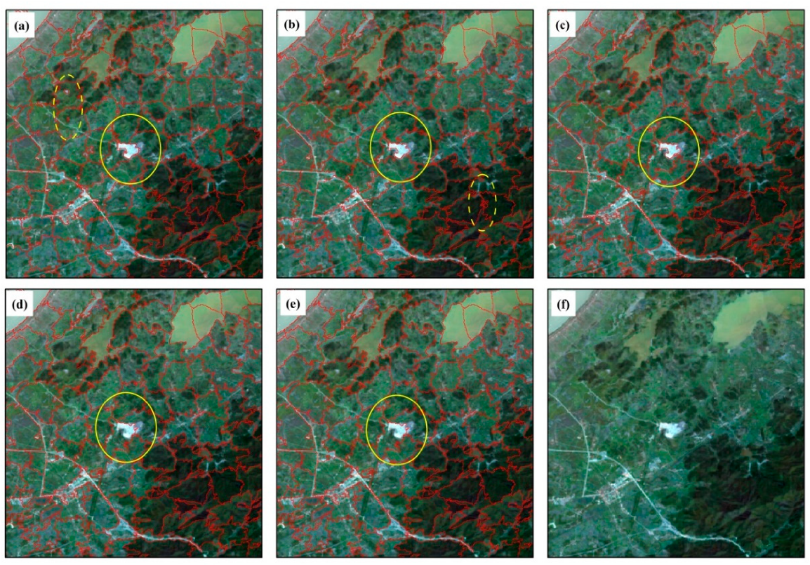
Different segmentation parameters further control the size and number of the satellite image objects, which may directly affect the classification results [8]. Therefore, our parameterization method, through visual comparison, may affect our classification results. Previous studies have shown that the uniform segmentation parameters are not the best for all LULC types [65]. To obtain the best segmentation results [23], we must attempt to separate the experiments on different LULC types. Here, this study proves that, due to the strong landscape heterogeneity, obtaining the best set of parameters suitable for all LULC types is impossible. To overcome this issue, we used the spectral standard deviation (STD) and maximum spectral distance from the original image to control the size of the generated image objects (Figure 9).
Based on Figure 9, when the STD is less than or equal to 0.25, the SNIC image segmentation algorithm can accurately detect the edges of ground objects. As shown in Figure 9a, when the STD is 0.15, some small pieces often appear in the image segmentation results. When the STD is 0.20, the small pieces are obviously reduced. However, in some mountainous area, there some small pieces still exist. In contrast, when the STD is greater than 0.25, the edges of the ground objects in the mixed region cannot be appropriately detected. Therefore, we uniformly set the STD to 0.25 in the image segmentation process.
As shown in Table 6, different STD settings result in different OAs. When no or few auxiliary features are added, the larger the value of the STD is set, the higher OA will be obtained. For the object-based models that only use spectral features, the highest OA is obtained when the STD is set to 0.35. With more auxiliary features added, the smaller the STD value the higher OA will be obtained. For the object-based models that use all auxiliary features, the OA is the highest when the STD is set to 0.15, but the classification result contains many small pieces. When the STD is set to 0.35, small ground objects cannot be classified. From the perspective of balancing OA and the fineness of classification results, the STD set to 0.25 is an optimal choice.
In the image segmentation process, we found that, except for grassland, the image segmentation results for cropland, forest, built-up land, and water body were satisfactory. The main reason for the poor image segmentation results for grassland is that the spectral characteristics of grassland are similar to cropland or forest. Therefore, distinguishing the boundaries of grassland with the spectral standard deviation is difficult. The optimal parameter settings for modeling different ground objects are usually not constant. However, the spectral standard deviation was set to 0.25, which yields the best ground object image segmentation results.
Except for the qualitative evaluation, we did not use quantitative methods to objectively evaluate our segmentation. Good image segmentation results are the prerequisite for efficient LULC classification because the objects and their attributes should be related to meaningful and coherent landscape features [13]. However, in our study area, for mixed and fuzzy LULC, delineating the boundaries between the objects is difficult, which may then affect the classification results.
Based on Figure 10, the overall results for image segmentation reflect the boundaries of the ground objects. However, as in Figure 10a,d, over-segmentation results exist in lakes and cultivated lands. Over-segmentation can generate a large number of image objects. When these small objects are classified, the object-based models take more computation time but there is no difference in classification accuracy. Therefore, although excessive segmentation exists in our image segmentation results, it has little effect on our research objectives and conclusions. In general, more image objects indicate ground object segmentation at a finer level, which leads to higher classification accuracy. However, more image objects require a stronger computation ability. In this study, we applied GEE, which can provide a powerful analysis platform for classification. Overall, over-segmentation in this study can improve the classification accuracy.
5.2. Pixel- versus Object-Based Methods for Landsat OLI Classification
Here, we compared the accuracy of the object- and pixel-based methods in LULC classification. Our results demonstrated that using the object-based method to classify Landsat OLI data can effectively improve the classification accuracy. Only using satellite data in the object-based RF classification methods yielded an OA of 94.04%. Combining spectral data with other types of auxiliary features under the object-based RF method can further improve the OA up to 96.01% (see Table 5).
We used Classification and Regression Trees (CART) to verify the generality and reliability of our conclusions [66]. In the comparative experiment, the features used in CART models were the same as RF models. The overall accuracy of CART classification is shown in Table 7. Results obtained from the CART models show that the OA is improved with the increase in the number of auxiliary features and the OAs of the object-based models are higher than those of the pixel-based models when the same features are used, which are consistent with the conclusions of the RF models.
The object-based method requires a significant amount of user processing, as well as increased computational capacity [67]. Therefore, considering a variety of auxiliary data for object-based classification in a large area is relatively time-consuming. Moreover, whether the object-based classification is useful for Landsat OLI data classification depends on the characteristics of the “object” in the study area. The object-based classification method requires more computing resources, especially when combined with multiple types of auxiliary features. However, the emergence of cloud computing platforms, such as GEE, enables access to powerful computing environments.
5.3. Uncertainties
Some studies have suggested that the training dataset should be as large as possible, especially when using machine learning classifiers (e.g., RF classifier) [68]. This is because the classification results are highly sensitive to the number, type ratio, and spatial autocorrelation of the training data [34]. Here, we generated the training data based on the multi-source LULC reference datasets. Therefore, the generated LULC types have certain ecological significance because they can be similar to the actual proportion of objects. Relative to the proportion of the ground truth, land types with few representations in the study area are usually underestimated. This may be because the classification tends to be biased towards the “most” available type in the training data [69]. We attempted to ensure that each LULC type had a sufficiently large sample size, and allocated samples according to the number of samples. Ensuring that all LULC types are represented by a sufficient number of samples is, however, still difficult due to the proportion of the ground truth. For instance, when generating the wetland and bare land sampling points, only 18 and 14 sample points were generated, respectively, which was too few for the overall number of sample points (18,878). We adjusted the sample distance from 1500 to 500 m, and the sample point number of wetlands and bare land were only 21 and 67, respectively, which is still too few for all of the sample points. Finally, we decided to exclude wetland and bare land types. Although reducing the number of LULC types may have an impact on the OA, the main LULC types in the study area still had a reasonably high OA.
6. Conclusions
In this study, we examined the effect that six auxiliary features in GEE had on accuracy improvements of 14 RF classification models (seven pixel-based RF models and seven object-based RF models); the main conclusions are:
(1) Auxiliary features, such as multiple remote sensing indices, topographic features, soil features, distance to the water sources, and phenological features, can improve the OA in heterogeneous landscapes. Landsat-8 OLI remote sensing image data were combined with the various auxiliary features used in this study, and we showed that they effectively improve the accuracy of LULC classification. The OA of the pixel-based (object-based) method increased from 91.51 to 94.20% (94.03 to 96.01%).
(2) The performance of the auxiliary features was not the same between pixel- and object-based models. In pixel-based models, soil features had the best effect on improving the classification accuracy. However, in object-based models, topographic features performed best. In the classification model combining all of the features, the topographic features had the greatest effect on improving the classification accuracy in both the pixel- and object-based models.
(3) We further found that when only using spectral data, the object-based classification method achieved higher OA and was unable to show small objects. Therefore, when object-based classification models are applied to medium resolution remote sensing images (such as Landsat data), other types of auxiliary features should be used.
The auxiliary data used in GEE in this study reflects a significant potential for improving the accuracy of LULC classifications in large areas with highly heterogeneous landscapes. However, we note that the main factors vary in different terrain areas. In the study, we used the YRD as a whole, and did not subdivide the YRD based on the terrain. In future studies, we will further investigate the similarities and differences in the optimal combination of auxiliary features under different topographic conditions.
Supplementary Materials
The following are available online at https://www.mdpi.com/2072-4292/13/3/453/s1, 1. Figure S1: Comparison of pixel-based classification results: (a)–(g) indicate M1–M7 model, respectively, Figure S2: Comparison of object-based classification results: (a)–(g) indicate M1’–M7’ model, respectively, Table S1: Relationships of land cover types in different land classification system, Table S2: Accuracy of M1–M7 RF models, Table S3: Accuracy of M1’–M7’ RF models, Table S4: Classification results by the 10 fold cross-validation models, Table S5: Time-costs of pixel and object-based models, Scripts for image pre-processing, Scripts for training points selection, Scripts for image segmentation, Scripts for image classification, accuracy assessment, and features’ importance.
Author Contributions
L.Q. designed and performed the experiments and wrote the draft; Z.C. designed the research and revised the manuscript; M.L. funded and supervised the research, and revised the manuscript; J.Z. designed the chart and revised the manuscript; H.W. preliminarily analyzed the results. All authors have read and agreed to the published version of the manuscript.
Funding
This research was funded by the National Key Research and Development Program of China, grant number 2017YFB0504205; the National Natural Science Foundation of China, grant number 41671386 and the Natural Science Research Project of Higher Education in Anhui Provence, and grant number KJ2020A0089.
Informed Consent Statement
Informed consent was obtained from all subjects involved in the study.
Data Availability Statement
The data used to support the findings of this study are available from the corresponding author upon request.
Conflicts of Interest
There is no conflict of interest. The funding sponsors had no role in the design of the study; in the collection, analyses, or interpretation of data; in the writing of the manuscript; and in the decision to publish the results.
References
- Dhanya, C.T.; Chaudhary, S. Dependence of Error Components in Satellite-Based Precipitation Products on Topography, LULC and Climatic Features. In American Geophysical Union, Fall Meeting 2018; Walter E Washingtion Convention Center: Washington, DC, USA, 2018. [Google Scholar]
- Disse, M.; Mekonnen, D.F.; Duan, Z.; Rientjes, T. Analysis of the Combined and Single Effects of LULC and Climate Change on the Streamflow of the Upper Blue Nile River Basin (UBNRB): Using Statistical Trend Tests, Remote Sensing Landcover Maps and the SWAT Model. Hydrol. Earth Syst. Sci. Discuss. 2018, 20, 18688. [Google Scholar]
- Rajbongshi, P.; Das, T.; Adhikari, D. Microenvironmental Heterogeneity Caused by Anthropogenic LULC Foster Lower Plant Assemblages in the Riparian Habitats of Lentic Systems in Tropical Floodplains. Sci. Total Environ. 2018, 639, 1254–1260. [Google Scholar] [CrossRef] [PubMed]
- Huang, H.; Chen, Y.; Clinton, N.; Wang, J.; Wang, X.; Liu, C.; Gong, P.; Yang, J.; Bai, Y.; Zheng, Y.; et al. Mapping Major Land Cover Dynamics in Beijing Using All Landsat Images in Google Earth Engine. Remote Sens. Environ. 2017, 202, 166–176. [Google Scholar] [CrossRef]
- Debats, S.R.; Luo, D.; Estes, L.D.; Fuchs, T.J.; Caylor, K.K. A Generalized Computer Vision Approach to Mapping Crop Fields in Heterogeneous Agricultural Landscapes. Remote Sens. Environ. 2016, 179, 210–221. [Google Scholar] [CrossRef] [Green Version]
- Klouček, T.; Moravec, D.; Komárek, J.; Lagner, O.; Štych, P. Selecting Appropriate Variables for Detecting Grassland to Cropland Changes Using High Resolution Satellite Data. PeerJ 2018, 6, e5487. [Google Scholar] [CrossRef] [PubMed]
- Phiri, D.; Morgenroth, J. Developments in Landsat Land Cover Classification Methods: A Review. Remote Sens. 2017, 9, 967. [Google Scholar] [CrossRef] [Green Version]
- Richards, J.A.; Landgrebe, D.A.; Swain, P.H. A Means for Utilizing Ancillary Information in Multispectral Classification. Remote Sens. Environ. 1982, 12, 463–477. [Google Scholar] [CrossRef]
- Ayala-Izurieta, J.E.; Márquez, C.O.; García, V.J.; Recalde-Moreno, C.G.; Rodríguez-Llerena, M.V.; Damián-Carrión, D.A. Land Cover Classification in an Ecuadorian Mountain Geosystem Using a Random Forest Classifier, Spectral Vegetation Indices, and Ancillary Geographic Data. Geosciences 2017, 7, 34. [Google Scholar] [CrossRef] [Green Version]
- Maxwell, A.E.; Strager, M.P.; Warner, T.A.; Ramezan, C.A.; Morgan, A.N.; Pauley, C.E. Large-Area, High Spatial Resolution Land Cover Mapping Using Random Forests, GEOBIA, and NAIP Orthophotography: Findings and Recommendations. Remote Sens. 2019, 11, 1409. [Google Scholar] [CrossRef] [Green Version]
- Corcoran, J.M.; Knight, J.F.; Gallant, A.L. Influence of Multi-Source and Multi-Temporal Remotely Sensed and Ancillary Data on the Accuracy of Random Forest Classification of Wetlands in Northern Minnesota. Remote Sens. 2013, 5, 3212–3238. [Google Scholar] [CrossRef] [Green Version]
- Jianya, G.; Haigang, S.; Guorui, M.; Qiming, Z. A Review of Multi-Temporal Remote Sensing Data Change Detection Algorithms. Int. Arch. Photogramm. Remote Sens. Spat. Inf. Sci. 2008, 37, 757–762. [Google Scholar]
- Xu, H. A New Index for Delineating Built-up Land Features in Satellite Imagery. Int. J. Remote Sens. 2008, 29, 4269–4276. [Google Scholar] [CrossRef]
- Liu, X.; Hu, G.; Chen, Y.; Li, X.; Xu, X.; Li, S.; Pei, F.; Wang, S. High-Resolution Multi-Temporal Mapping of Global Urban Land Using Landsat Images Based on the Google Earth Engine Platform. Remote Sens. Environ. 2018, 209, 227–239. [Google Scholar] [CrossRef]
- Bruzzone, L.; Prieto, D.F. An Adaptive Semiparametric and Context-Based Approach to Unsupervised Change Detection in Multitemporal Remote-Sensing Images. IEEE Trans. Image Process. 2002, 11, 452–466. [Google Scholar] [CrossRef]
- Viana, C.M.; Girão, I.; Rocha, J. Long-Term Satellite Image Time-Series for Land Use/Land Cover Change Detection Using Refined Open Source Data in a Rural Region. Remote Sens. 2019, 11, 1104. [Google Scholar] [CrossRef] [Green Version]
- Shen, W.; Li, M.; Wei, A. Spatio-Temporal Variations in Plantation Forests’ Disturbance and Recovery of Northern Guangdong Province Using Yearly Landsat Time Series Observations (1986–2015). Chin. Geogr. Sci. 2017, 27, 600–613. [Google Scholar] [CrossRef]
- Franklin, S.E. Ancillary Data Input to Satellite Remote Sensing of Complex Terrain Phenomena. Comput. Geosci. 1989, 15, 799–808. [Google Scholar] [CrossRef]
- Gorelick, N.; Hancher, M.; Dixon, M.; Ilyushchenko, S.; Thau, D.; Moore, R. Google Earth Engine: Planetary-Scale Geospatial Analysis for Everyone. Remote Sens. Environ. 2017, 202, 18–27. [Google Scholar] [CrossRef]
- Zhou, B.; Okin, G. Leveraging Google Earth Engine (GEE) to Model Large-Scale Land Cover Dynamics in Western US. AGUFM 2018, 2018, B41N-2907. [Google Scholar]
- Franklin, S.E. Pixel- and Object-Based Multispectral Classification of Forest Tree Species from Small Unmanned Aerial Vehicles. J. Unmanned Veh. Syst. 2018, 6, 195–211. [Google Scholar] [CrossRef] [Green Version]
- Berhane, T.; Lane, C.; Wu, Q.; Anenkhonov, O.; Chepinoga, V.; Autrey, B.; Liu, H. Comparing Pixel- and Object-Based Approaches in Effectively Classifying Wetland-Dominated Landscapes. Remote Sens. 2017, 10, 46. [Google Scholar] [CrossRef] [PubMed] [Green Version]
- Ye, S.; Pontius, R.G.; Rakshit, R. A Review of Accuracy Assessment for Object-Based Image Analysis: From Per-Pixel to Per-Polygon Approaches. ISPRS J. Photogramm. Remote Sens. 2018, 141, 137–147. [Google Scholar] [CrossRef]
- Chen, Y.; Zhou, Y.; Ge, Y.; An, R.; Chen, Y. Enhancing Land Cover Mapping through Integration of Pixel-Based and Object-Based Classifications from Remotely Sensed Imagery. Remote Sens. 2018, 10, 77. [Google Scholar] [CrossRef] [Green Version]
- Zheng, Y.; Wu, J.; Wang, A.; Chen, J. Object- and Pixel-Based Classifications of Macroalgae Farming Area with High Spatial Resolution Imagery. Geocarto Int. 2018, 33, 1048–1063. [Google Scholar] [CrossRef]
- Estoque, R.C.; Murayama, Y.; Akiyama, C.M. Pixel-Based and Object-Based Classifications Using High- and Medium-Spatial-Resolution Imageries in the Urban and Suburban Landscapes. Geocarto Int. 2015, 30, 1113–1129. [Google Scholar] [CrossRef] [Green Version]
- Gu, C.; Hu, L.; Zhang, X.; Wang, X.; Guo, J. Climate Change and Urbanization in the Yangtze River Delta. Habitat Int. 2011, 35, 544–552. [Google Scholar] [CrossRef]
- Cai, W.; Gibbs, D.; Zhang, L.; Ferrier, G.; Cai, Y. Identifying Hotspots and Management of Critical Ecosystem Services in Rapidly Urbanizing Yangtze River Delta Region, China. J. Environ. Manag. 2017, 191, 258–267. [Google Scholar] [CrossRef]
- Li, Y.; Wu, F. Understanding City-Regionalism in China: Regional Cooperation in the Yangtze River Delta. Reg. Stud. 2018, 52, 313–324. [Google Scholar] [CrossRef]
- Wang, Y.; Xu, Y.; Tabari, H.; Wang, J.; Wang, Q.; Song, S.; Hu, Z. Innovative Trend Analysis of Annual and Seasonal Rainfall in the Yangtze River Delta, Eastern China. Atmos. Res. 2020, 231, 104673. [Google Scholar] [CrossRef]
- Shen, S.; Yue, P.; Fan, C. Quantitative Assessment of Land Use Dynamic Variation Using Remote Sensing Data and Landscape Pattern in the Yangtze River Delta, China. Sustain. Comput. Inform. Syst. 2019, 23, 111–119. [Google Scholar] [CrossRef]
- Jin, Y.; Liu, X.; Yao, J.; Zhang, X.; Zhang, H. Mapping the Annual Dynamics of Cultivated Land in Typical Area of the Middle-Lower Yangtze Plain Using Long Time-Series of Landsat Images Based on Google Earth Engine. Int. J. Remote Sens. 2020, 41, 1625–1644. [Google Scholar] [CrossRef]
- Pareeth, S.; Karimi, P.; Shafiei, M.; De Fraiture, C. Mapping Agricultural Landuse Patterns from Time Series of Landsat 8 Using Random Forest Based Hierarchial Approach. Remote Sens. 2019, 11, 601. [Google Scholar] [CrossRef] [Green Version]
- Millard, K.; Richardson, M. On the Importance of Training Data Sample Selection in Random Forest Image Classification: A Case Study in Peatland Ecosystem Mapping. Remote Sens. 2015, 7, 8489–8515. [Google Scholar] [CrossRef] [Green Version]
- Sulla-Menashe, D.; Friedl, M.A. User Guide to Collection 6 MODIS Land Cover (MCD12Q1 and MCD12C1) Product; USGS: Reston, VA, USA, 2018.
- Arino, O.; Ramos Perez, J.; Kalogirou, V.; Bontemps, S.; Defourny, P.; van Bogaert, E. Global Land Cover Map for 2009 (GlobCover 2009); European Space Agency (ESA) & Université Catholique de Louvain (UCL): Frascati, Italy, 2012. [Google Scholar]
- Rodriguez-Galiano, V.; Chica-Olmo, M. Land Cover Change Analysis of a Mediterranean Area in Spain Using Different Sources of Data: Multi-Seasonal Landsat Images, Land Surface Temperature, Digital Terrain Models and Texture. Appl. Geogr. 2012, 35, 208–218. [Google Scholar] [CrossRef]
- Aredehey, G.; Mezgebu, A.; Girma, A. Land-Use Land-Cover Classification Analysis of Giba Catchment Using Hyper Temporal MODIS NDVI Satellite Images. Int. J. Remote Sens. 2018, 39, 810–821. [Google Scholar] [CrossRef]
- Atzberger, C.; Rembold, F. Mapping the Spatial Distribution of Winter Crops at Sub-Pixel Level Using AVHRR NDVI Time Series and Neural Nets. Remote Sens. 2013, 5, 1335–1354. [Google Scholar] [CrossRef] [Green Version]
- Lu, D.; Chen, Q.; Wang, G.; Liu, L.; Li, G.; Moran, E. A Survey of Remote Sensing-Based Aboveground Biomass Estimation Methods in Forest Ecosystems. Int. J. Digit. Earth 2016, 9, 63–105. [Google Scholar] [CrossRef]
- Crist, E.P.; Cicone, R.C. A Physically-Based Transformation of Thematic Mapper Data—The TM Tasseled Cap. IEEE Trans. Geosci. Remote Sens. 1984, GE-22, 256–263. [Google Scholar] [CrossRef]
- Füreder, P. Topographic Correction of Satellite Images for Improved LULC Classification in Alpine Areas. Grazer Schr. Geogr. Raumforsch. 2010, 45, 187–194. [Google Scholar]
- Gao, Y.; Zhang, W. LULC Classification and Topographic Correction of Landsat-7 ETM+ Imagery in the Yangjia River Watershed: The Influence of DEM Resolution. Sensors 2009, 9, 1980–1995. [Google Scholar] [CrossRef] [Green Version]
- Wang, C.; Jia, M.; Chen, N.; Wang, W. Long-Term Surface Water Dynamics Analysis Based on Landsat Imagery and the Google Earth Engine Platform: A Case Study in the Middle Yangtze River Basin. Remote Sens. 2018, 10, 1635. [Google Scholar] [CrossRef] [Green Version]
- Bi, L.; Fu, B.L.; Lou, P.Q.; Tang, T.Y. Delineation Water of Pearl River Basin Using Landsat Images from Google Earth Engine. ISPRS Int. Arch. Photogramm. Remote Sens. Spat. Inf. Sci. 2020, XLII-3/W10, 5–10. [Google Scholar] [CrossRef] [Green Version]
- Kim, G.; Barros, A.P. Downscaling of Remotely Sensed Soil Moisture with a Modified Fractal Interpolation Method Using Contraction Mapping and Ancillary Data. Remote Sens. Environ. 2002, 83, 400–413. [Google Scholar] [CrossRef]
- Hengl, T.; de Jesus, J.M.; Heuvelink, G.B.; Gonzalez, M.R.; Kilibarda, M.; Blagotić, A.; Shangguan, W.; Wright, M.N.; Geng, X.; Bauer-Marschallinger, B. SoilGrids250m: Global Gridded Soil Information Based on Machine Learning. PLoS ONE 2017, 12, e0169748. [Google Scholar] [CrossRef] [Green Version]
- Chen, B.; Xiao, X.; Wu, Z.; Yun, T.; Kou, W.; Ye, H.; Lin, Q.; Doughty, R.; Dong, J.; Ma, J.; et al. Identifying Establishment Year and Pre-Conversion Land Cover of Rubber Plantations on Hainan Island, China Using Landsat Data during 1987–2015. Remote Sens. 2018, 10, 1240. [Google Scholar] [CrossRef] [Green Version]
- Hu, Y.; Hu, Y. Land Cover Changes and Their Driving Mechanisms in Central Asia from 2001 to 2017 Supported by Google Earth Engine. Remote Sens. 2019, 11, 554. [Google Scholar] [CrossRef] [Green Version]
- Breiman, L. Random Forests. Mach. Learn. 2001, 45, 5–32. [Google Scholar] [CrossRef] [Green Version]
- Silveira, E.M.O.; Silva, S.H.G.; Acerbi-Junior, F.W.; Carvalho, M.C.; Carvalho, L.M.T.; Scolforo, J.R.S.; Wulder, M.A. Object-Based Random Forest Modelling of Aboveground Forest Biomass Outperforms a Pixel-Based Approach in a Heterogeneous and Mountain Tropical Environment. Int. J. Appl. Earth Obs. Geoinf. 2019, 78, 175–188. [Google Scholar] [CrossRef]
- Pelletier, C.; Valero, S.; Inglada, J.; Champion, N.; Sicre, C.M.; Dedieu, G. Effect of Training Class Label Noise on Classification Performances for Land Cover Mapping with Satellite Image Time Series. Remote Sens. 2017, 9, 173. [Google Scholar] [CrossRef] [Green Version]
- Yan, L.; Roy, D.P. Improved Time Series Land Cover Classification by Missing-Observation-Adaptive Nonlinear Dimensionality Reduction. Remote Sens. Environ. 2015, 158, 478–491. [Google Scholar] [CrossRef] [Green Version]
- Pelletier, C.; Valero, S.; Inglada, J.; Champion, N.; Dedieu, G. Assessing the Robustness of Random Forests to Map Land Cover with High Resolution Satellite Image Time Series over Large Areas. Remote Sens. Environ. 2016, 187, 156–168. [Google Scholar] [CrossRef]
- Liaw, A.; Wiener, M. Classification and Regression by RandomForest. R News 2002, 2, 18–22. [Google Scholar]
- Belgiu, M.; Drăguţ, L. Random Forest in Remote Sensing: A Review of Applications and Future Directions. ISPRS J. Photogramm. Remote Sens. 2016, 114, 24–31. [Google Scholar] [CrossRef]
- Achanta, R.; Susstrunk, S. Superpixels and Polygons Using Simple Non-Iterative Clustering. In Proceedings of the IEEE Conference on Computer Vision and Pattern Recognition, Honolulu, HI, USA, 21–26 July 2017; pp. 4651–4660. [Google Scholar]
- Xiong, J.; Thenkabail, P.; Tilton, J.; Gumma, M.; Teluguntla, P.; Oliphant, A.; Congalton, R.; Yadav, K.; Gorelick, N. Nominal 30-m Cropland Extent Map of Continental Africa by Integrating Pixel-Based and Object-Based Algorithms Using Sentinel-2 and Landsat-8 Data on Google Earth Engine. Remote Sens. 2017, 9, 1065. [Google Scholar] [CrossRef] [Green Version]
- Stromann, O.; Nascetti, A.; Yousif, O.; Ban, Y. Dimensionality Reduction and Feature Selection for Object-Based Land Cover Classification Based on Sentinel-1 and Sentinel-2 Time Series Using Google Earth Engine. Remote Sens. 2020, 12, 76. [Google Scholar] [CrossRef] [Green Version]
- Salehi, B.; Zhang, Y.; Zhong, M. A Combined Object- and Pixel-Based Image Analysis Framework for Urban Land Cover Classification of VHR Imagery. Photogramm. Eng. Remote Sens. 2013, 79, 999–1014. [Google Scholar] [CrossRef]
- Keyport, R.N.; Oommen, T.; Martha, T.R.; Sajinkumar, K.S.; Gierke, J.S. A Comparative Analysis of Pixel- and Object-Based Detection of Landslides from Very High-Resolution Images. Int. J. Appl. Earth Obs. Geoinf. 2018, 64, 1–11. [Google Scholar] [CrossRef]
- Fox, E.W.; Hill, R.A.; Leibowitz, S.G.; Olsen, A.R.; Thornbrugh, D.J.; Weber, M.H. Assessing the Accuracy and Stability of Variable Selection Methods for Random Forest Modeling in Ecology. Environ. Monit. Assess. 2017, 189, 316. [Google Scholar] [CrossRef]
- Jastrzębski, S.; Leśniak, D.; Czarnecki, W.M. Learning to SMILE(S). arXiv 2018, arXiv:1602.06289. [Google Scholar]
- Gregorutti, B.; Michel, B.; Saint-Pierre, P. Correlation and Variable Importance in Random Forests. Stat. Comput. 2017, 27, 659–678. [Google Scholar] [CrossRef] [Green Version]
- Myint, S.W.; Gober, P.; Brazel, A.; Grossman-Clarke, S.; Weng, Q. Per-Pixel vs. Object-Based Classification of Urban Land Cover Extraction Using High Spatial Resolution Imagery. Remote Sens. Environ. 2011, 115, 1145–1161. [Google Scholar] [CrossRef]
- Zhou, Z.; Ma, L.; Fu, T.; Zhang, G.; Yao, M.; Li, M. Change Detection in Coral Reef Environment Using High-Resolution Images: Comparison of Object-Based and Pixel-Based Paradigms. ISPRS Int. J. Geo-Inf. 2018, 7, 441. [Google Scholar] [CrossRef] [Green Version]
- Costa, H.; Carrão, H.; Bação, F.; Caetano, M. Combining Per-Pixel and Object-Based Classifications for Mapping Land Cover over Large Areas. Int. J. Remote Sens. 2014, 35, 738–753. [Google Scholar] [CrossRef]
- Salehi, B.; Chen, Z.; Jefferies, W.; Adlakha, P.; Bobby, P.; Power, D. Well Site Extraction from Landsat-5 TM Imagery Using an Object- and Pixel-Based Image Analysis Method. Int. J. Remote Sens. 2014, 35, 7941–7958. [Google Scholar] [CrossRef]
- Zhou, F.; Zhang, A. Optimal Subset Selection of Time-Series MODIS Images and Sample Data Transfer with Random Forests for Supervised Classification Modelling. Sensors 2016, 16, 1783. [Google Scholar] [CrossRef] [Green Version]
Figure 1.
Location of the Yangtze River Delta (YRD) region in China.

Figure 2.
Datasets used in the study: (A) Median of the 2015 Landsat 8 Operational Land Imager (OLI) (4/3/2 bands), (B) Max Normalized Difference Vegetation Index (NDVI), (C,D) Shuttle Radar Topography Mission (SRTM) Digital Elevation Data, (E) European Commission’s Joint Research Centre (JRC) Yearly Water Classification History, and (F) OpenLandMap SoilGrids.

Figure 3.
Flowchart describing the data processing and analysis steps, including sample selection, image segmentation, random forest (RF) classification, classification accuracy assessment, and mechanism analysis.
Figure 3.
Flowchart describing the data processing and analysis steps, including sample selection, image segmentation, random forest (RF) classification, classification accuracy assessment, and mechanism analysis.

Figure 4.
Most important features in the pixel-based models.

Figure 5.
Most important features in the object-based models.

Figure 6.
Comparison of the pixel-based classification results in a typical region. M1–M7 indicate the classification results of the seven pixel-based models listed in Table 3, respectively. The central subfigure is Landsat 8 OLI true color image.
Figure 6.
Comparison of the pixel-based classification results in a typical region. M1–M7 indicate the classification results of the seven pixel-based models listed in Table 3, respectively. The central subfigure is Landsat 8 OLI true color image.

Figure 7.
Comparison of the object-based classification results in a typical region. M1’–M7’ indicate the classification results of the seven object-based models listed in Table 3, respectively. The central subfigure is Landsat 8 OLI true color image.
Figure 7.
Comparison of the object-based classification results in a typical region. M1’–M7’ indicate the classification results of the seven object-based models listed in Table 3, respectively. The central subfigure is Landsat 8 OLI true color image.

Figure 8.
Comparison of all the feature classification results of the pixel- and object-based models. The image on the left is a Landsat-8 OLI true color composite with the A1 and A2 areas. (a) Result of the all features classification of the pixel-based model. (b) Result of the all features classification of the object-based model.

Figure 9.
Image segmentation results for different spectral standard deviations in a typical area. The spectral standard deviations are (a) 0.15, (b) 0.20, (c) 0.25, (d) 0.30, and (e) 0.35. (f) The Landsat-8 OLI true color composite.
Figure 9.
Image segmentation results for different spectral standard deviations in a typical area. The spectral standard deviations are (a) 0.15, (b) 0.20, (c) 0.25, (d) 0.30, and (e) 0.35. (f) The Landsat-8 OLI true color composite.

Figure 10.
Landsat 8 (Green: band 4, Red: band 3, and Blue: band 2) with segmentation objects overlaid in a typical area: (a) lakes, (b) forests, (c) built-up areas, and (d) cultivated lands.
Figure 10.
Landsat 8 (Green: band 4, Red: band 3, and Blue: band 2) with segmentation objects overlaid in a typical area: (a) lakes, (b) forests, (c) built-up areas, and (d) cultivated lands.


Table 1.
Datasets used in this study.
| Data | Spatial Resolution | Data Format | Temporal Coverage | Usage |
|---|---|---|---|---|
| Landsat 8 OLI * | 30 m | GeoTiff | 2015 | Land use classification |
| MODIS12Q1. 006 * | 500 m | GeoTiff | 2008–2015 | Creative land use samples |
| GlobCover * | 300 m | GeoTiff | 2009 | Creative land use samples |
| JRC Yearly Water Classification History * | 30 m | GeoTiff | 2015 | Water data |
| SRTM Digital Elevation Data * | 30 m | GeoTiff | 2009 | Elevation data |
| OpenLandMap Soil v02 * | 250 m | GeoTiff | 2017 | Soil data |
| Land Survey Data | 1:10,000 | Shapefile | 2008, 2010 | Creation and validation samples |
| Administrative boundary data | 1:10,000 | Shapefile | 2015 | Determination of the YRD boundaries |
Note that JRC: European Commission’s Joint Research Centre; SRTM: Shuttle Radar Topography Mission; * available online at https://earthengine.google.com.
Table 2.
Features in the land use/land cover (LULC) classification.
| Features, Number of Features | Description | Data Source |
|---|---|---|
| spectral features (12) | Median of bands 2–7. Median of principal components 2–7. | Landsat-8 OLI |
| spectral indices (20) | Median and max of the NDVI, NDWI, NDBI, NBR, NDMI, SAVI, TCB, TCG, TCW, and TCA. | Landsat-8 OLI |
| topographic features (3) | Median of the elevation, slope, and aspect. | Shuttle Radar Topography Mission |
| distance to water bodies (1) | Euclidean distance to water bodies. | European Commission’s Joint Research Centre |
| soil features (31) | Median of a soil organic carbon stock and content; pH of H2O, sand, silt, and clay content; water content; bulk density of the fine earth fraction; cation exchange capacity; and proportion of coarse fragments. | OpenLandMap |
| spectral–temporal metrics (27) | Max, min and median of bands 2–7, NDVI, NDWI, and NDBI. | Landsat-8 OLI |
Note that NDVI: Normalized Difference Vegetation Index; NDWI: Normalized Difference Water Index; NDBI: Normalized Difference Build-up Index; NBR: Normalized Burn Ratio; NDMI: Normalized Difference Moisture Index; SAVI: Soil Adjusted Vegetation Index; TCB: Tasselled Cap Brightness; TCG: Tasselled Cap Greenness; TCW: Tasselled Cap Wetness; and TCA: Tasselled Cap Angle.
Table 3.
Models used in this study for LULC classification.
| Models | Description | Auxiliary Features Used |
|---|---|---|
| M1 | Pixel-based spectral features classification model | Spectral features |
| M1’ | Object-based spectral features classification model | Spectral features |
| M2 | Pixel-based spectral features + spectral index classification model | Spectral indices |
| M2’ | Object-based spectral features + spectral index classification model | Spectral indices |
| M3 | Pixel-based spectral features + topographic features classification model | Topographic features |
| M3’ | Object-based spectral features + topographic features classification model | Topographic features |
| M4 | Pixel-based spectral features + distance to water body classification model | Distance to water bodies |
| M4’ | Object-based spectral features + distance to water body classification model | Distance to water bodies |
| M5 | Pixel-based spectral features + soil features classification model | Soil features |
| M5’ | Object-based spectral features + soil features classification model | Soil features |
| M6 | Pixel-based spectral features + spectral–temporal metrics classification model | Spectral–temporal metrics |
| M6’ | Object-based spectral features + spectral–temporal metrics classification model | Spectral–temporal metrics |
| M7 | Pixel-based all features classification model | All features |
| M7’ | Object-based all features classification model | All features |
Table 4.
Accuracy results for the pixel-based classification models.
| M1 | M2 | M3 | M4 | M5 | M6 | M7 | |
|---|---|---|---|---|---|---|---|
| Kappa | 0.87 | 0.89 | 0.89 | 0.89 | 0.90 | 0.89 | 0.91 |
| Overall accuracy (%) | 91.51 | 92.73 | 92.36 | 92.62 | 93.53 | 92.73 | 94.20 |
Table 5.
Accuracy results for the object-based classification models.
| M1’ | M2’ | M3’ | M4’ | M5’ | M6’ | M7’ | |
|---|---|---|---|---|---|---|---|
| Kappa | 0.91 | 0.92 | 0.94 | 0.92 | 0.93 | 0.93 | 0.94 |
| Overall accuracy (%) | 94.03 | 94.67 | 95.73 | 94.91 | 95.27 | 94.95 | 96.01 |
Table 6.
The object-based classification overall accuracies by different spectral standard deviation.
Table 6.
The object-based classification overall accuracies by different spectral standard deviation.
| Auxiliary Features Used | Spectral Standard Deviation | ||||
|---|---|---|---|---|---|
| 0.15 | 0.20 | 0.25 | 0.30 | 0.35 | |
| spectral features | 94.26 | 94.09 | 94.03 | 94.14 | 94.49 |
| spectral indices | 94.61 | 95.26 | 94.67 | 95.08 | 94.48 |
| topographic features | 95.57 | 95.82 | 95.73 | 95.61 | 95.90 |
| distance to water bodies | 94.73 | 95.07 | 94.91 | 94.65 | 94.96 |
| soil features | 95.40 | 95.17 | 95.27 | 94.77 | 94.72 |
| spectral–temporal metrics | 95.37 | 95.14 | 94.95 | 94.72 | 95.31 |
| ALL | 96.23 | 95.92 | 96.01 | 95.74 | 95.91 |
Table 7.
Overall accuracy results of the Classification and Regression Trees (CART) models.
| Auxiliary Features Used | Pixel-Based | Object-Based |
|---|---|---|
| spectral features | 86.55 | 90.96 |
| spectral indices | 87.79 | 91.40 |
| topographic features | 88.34 | 93.07 |
| distance to water bodies | 88.09 | 91.50 |
| soil features | 90.12 | 92.24 |
| spectral–temporal metrics | 88.01 | 92.55 |
| ALL | 91.26 | 93.37 |
Publisher’s Note: MDPI stays neutral with regard to jurisdictional claims in published maps and institutional affiliations. |
© 2021 by the authors. Licensee MDPI, Basel, Switzerland. This article is an open access article distributed under the terms and conditions of the Creative Commons Attribution (CC BY) license (http://creativecommons.org/licenses/by/4.0/).
Share and Cite
MDPI and ACS Style
Qu, L.; Chen, Z.; Li, M.; Zhi, J.; Wang, H. Accuracy Improvements to Pixel-Based and Object-Based LULC Classification with Auxiliary Datasets from Google Earth Engine. Remote Sens. 2021, 13, 453. https://doi.org/10.3390/rs13030453
AMA Style
Qu L, Chen Z, Li M, Zhi J, Wang H. Accuracy Improvements to Pixel-Based and Object-Based LULC Classification with Auxiliary Datasets from Google Earth Engine. Remote Sensing. 2021; 13(3):453. https://doi.org/10.3390/rs13030453
Chicago/Turabian StyleQu, Le’an, Zhenjie Chen, Manchun Li, Junjun Zhi, and Huiming Wang. 2021. "Accuracy Improvements to Pixel-Based and Object-Based LULC Classification with Auxiliary Datasets from Google Earth Engine" Remote Sensing 13, no. 3: 453. https://doi.org/10.3390/rs13030453
Note that from the first issue of 2016, this journal uses article numbers instead of page numbers. See further details here.