
Remote 3D Displacement Sensing for Large Structures with Stereo Digital Image Correlation

1
College of Civil Engineering and Architecture, Zhejiang University of Water Resources and Electric Power, Hangzhou 310018, China
2
Shanghai Key Laboratory of Mechanics in Energy Engineering, Shanghai Institute of Applied Mathematics and Mechanics, School of Mechanics and Engineering Science, Shanghai University, Shanghai 200444, China
*
Author to whom correspondence should be addressed.
Remote Sens. 2023, 15(6), 1591; https://doi.org/10.3390/rs15061591
Submission received: 9 February 2023
/
Revised: 10 March 2023
/
Accepted: 13 March 2023
/
Published: 15 March 2023
(This article belongs to the Special Issue Remote Sensing in Structural Health Monitoring)
Abstract
:The work performance of stereo digital image correlation (stereo-DIC) technologies, especially the operating accuracy and reliability in field applications, is not fully understood. In this study, the key technologies of the field remote 3D displacement sensing of civil structures based on stereo-DIC have been proposed. An image correlation algorithm is incorporated in improving the matching accuracy of control points. An adaptive stereo-DIC extrinsic parameter calibration method is developed by fusing epipolar-geometry-based and homography-based methods. Furthermore, a reliable reference frame that does not require artificial markers is established based on Euclidean transformation, which facilitates in-plane and out-of-plane displacement monitoring for civil structures. Moreover, a camera motion correction is introduced by considering background points according to the camera motion model. With an experiment, the feasibility and accuracy of the proposed system are validated. Moreover, the system is applied to sense the dynamic operating displacement of a 2 MW wind turbine’s blades. The results show the potential capability of the proposed stereo-DIC system in remote capturing the full-field 3D dynamic responses and health status of large-scale structures.

1. Introduction
The structural health monitoring (SHM) of civil structures is important for insuring service quality and safety [1,2]. Limited to the traditional displacement monitoring technologies (e.g., LVDT, GNSS, displacement sensor, etc.) that are inevitably embedded in a structure, non-contact monitoring techniques are of great interest to engineering societies [3,4]. Due to the advantages of simple instrumentation and installation (remote operation and full-field measurement capacity), the existing literature has indicated the potential of digital image correlation (DIC)-based monitoring methods for SHM [5,6].
At present, 2D digital image correlation (2D-DIC) based on monocular cameras is used to measure the in-plane deformation of materials and civil structures [7,8,9,10]. Earlier, in 2011, Maier et al. used the technique to identify the material parameters of concrete and, combined with the finite element model, evaluate the operational condition of concrete dams [11]. Based on that study, Gajewski et al. obtained the essential material parameters of multiple materials including concrete, polyurethane foams, and paper foils using an optimized 2D-DIC technique and inverse analysis [12,13,14,15]. Nevertheless, the out-of-plane deformation is unable to be measured by the 2D-DIC method, which is important for the health monitoring of certain structures, such as high-rise buildings, transmission towers, cranes, etc. The stereo-DIC technique is capable of estimating the 3D deformation of the region of interest (ROI) by acquiring image pairs from different view angles of the structure under test loading. It has been applied to estimate the compressive stiffness and strength of corrugated cardboard [16,17]. In addition, the technology offers a promising method of 3D-displacement measurement and has received increasing attention in SHM [18,19].
In lab conditions, the matching accuracy of DIC can meet a range of 0.02–0.20 pixels [20]. However, measurement accuracy and robustness remain headaches in uncontrollable field conditions. Among them, the major critical challenges are system parameter calibration, reference frame establishment, and camera motion correction.
1.1. Calibration of Extrinsic Parameters for Stereo-DIC
Stereo-DIC calibration aims to determine intrinsic parameters, including the principal point, distortion coefficients, and focal lengths, and the extrinsic parameters of relative translation and rotation. The intrinsic parameters of each camera are usually calibrated in the laboratory; however, the extrinsic parameters cannot be pre-calibrated, as they often vary with the arrangement of the measurement system.
Camera calibration methods can be roughly divided into two classifications: photogrammetric calibration and self-calibration. It is a well-established photogrammetric calibration technique to calibrate stereo cameras with known targets [21,22]. The known pattern in the targets allows us to obtain both the intrinsic and extrinsic parameters at a remarkably high accuracy. For a large field of view (FOV) measurement, it is difficult to apply a regular-sized calibration target, and the cost of fabricating a large target is expensive. A self-calibration method based on a 3D point array only needs a constraint from the image sequence without the need to design any special reference patterns in advance [23]. However, as the uniformly distributed and stable features in field applications are not always available, measurement accuracy is accordingly not always guaranteed.
Some innovative calibration techniques, such as a CAD-based method [24], a projection-based method [25,26,27], a combination of multiple small chessboards [28], and a speckle-based method [29], have been developed. Although successful in applications, the calibration accuracy and flexibility should be further improved due to three challenges: (1) high-precision equipment or image-stitching algorithms are needed for large FOVs; (2) a lack of control points limits applications of stereo-DIC; and (3) unstable feature extraction and matching causes errors in camera calibration in field applications.
1.2. Establishment of Reference Frame for Stereo-DIC
Three-dimensional displacement components are usually measured in a given coordinate system. However, few studies are available on how to set up the reference frame in stereo-DIC. Generally, the reference frame of a stereo-DIC is aligned with the left camera frame. However, the actual in-plane and out-of-plane deformations of a structure usually differ from the reference frame. Therefore, coordinate transform is expected after the orientation of the in-plane and out-of-plane of the object is determined [30].
In most of the previous works, the frame alignment was achieved by installing ancillary equipment on the measured object [31]. On the one hand, the method requires high-precision equipment to process the reference tool, but on the other hand, a special structure needs to be designed to strictly ensure the rigid connection between the measured object and the tool. Therefore, the methods inevitably affect the structure and deformation characteristics of the measured structure itself, which has disadvantages such as high costs and unreliable deformation data.
1.3. Camera Motion Correction
Camera motion is a key factor affecting the accuracy of stereo-DIC in field applications since the imaging units are usually mounted tripods [32]. Compared with laboratory conditions, it is more difficult to make the cameras remain fixed in the field due to the existence of wind and ground vibrations [33]. Any slight camera motion can directly lead to a change in the extrinsic parameters and potentially cause errors in the 3D reconstruction. Therefore, the correction of camera motion is crucial to accurate stereo-DIC measurements in-field.
A common correction treatment is to use auxiliary devices [34,35,36,37]. However, the methods are not feasible in-field due to the inconvenience of installing devices. To simplify the operation, stationary background points (BG points) are also considered in camera motion correction. Chen et al. estimated the camera′s motion signal using BG points in the frame that were assumed to be static [38]. Abolhasannejad et al. defined a region of interest in the background of the reference image and developed an affine motion estimator to calculate the global motion parameters [39]. Yoon et al. estimated the 6-DOF camera’s motion by tracking the BG points and measured the absolute 2D displacement of the structure [40]. Although the above studies used background information, the out-of-plane motion of the interested points was not compensated. Since the existing research has focused on monocular camera motion correction, challenges for camera motion correction for stereo-DIC remain.
To address the above limitations, we propose several techniques to improve the performance of stereo-DIC measurement in field applications. An image correlation algorithm is introduced to the matching of control points, and then, an adaptive stereo-DIC extrinsic parameters calibration method is developed in Section 2.2. A reference frame is established based on Euclidean transformation to realize in- and out-of-plane displacement estimation in Section 2.3. A camera motion correction based on motion model parameters is proposed in Section 2.4. We evaluate the accuracy and feasibility of the proposed stereo-DIC system and techniques using an experiment in Section 3.2. The operating state of a 2 MW wind turbine is preliminarily evaluated using the established system in Section 3.3. Discussions are presented in Section 4, and Section 5 is the conclusion.
2. Methodology
2.1. Working Procedure
Figure 1 shows a flowchart of civil structure displacement measurement based on a stereo-DIC system. The process is divided into 5 steps.
Step 1: Assemble the system and capture reference images. A stereo-DIC system was used to capture a set of reference images. In this study, a binocular stereo-vision system was employed to record images. A synchronization signal is introduced to enable simultaneous image pair acquisition. Since the system is designed for 3D measurement for large structures, cameras are mounted on individual tripods, and camera calibration is a key procedure to ensure precise 3D displacement measurements. For a large FOV, the precise chessboard method, which is widely used in laboratories, is no longer effective due to its limited geometric size. Camera calibration is usually completed in a two-stage routine. The intrinsic parameters of each imaging unit are predetermined using a chessboard based on Zhang’s method. The extrinsic parameters are determined after the dual imaging system is set up in the field. Feature points, whose image coordinates can be determined in the left and right images, are extracted to complete the follow-up camera calibration operation. Thus, in this step, the distance between the dual cameras is measured and pairs of reference images are simultaneously recorded.
Step 2: Calibrate stereo camera parameters. Speeded-Up Robust Features (SURF) is employed to recognize and match feature points in the image pairs. An image correlation algorithm is also introduced to the feature-matching process to filter out the incorrect feature points. The image coordinate pairs of the extracted feature points are randomly divided into 2 groups. The majority is used for camera calibration and the rest are for estimating re-projection errors. Typical camera calibration methods, including epipolar-geometry-based and homography-based calibrations, are conducted. The parameters corresponding to small re-projection errors are selected as the optimal solution for the extrinsic parameters.
Step 3: Establish a reference frame. After camera calibration, the reference frame is aligned by default with the coordinate frame of the left camera. This coordinate system is inconvenient for the displacement analysis of the structure. A reference frame that coincides with the displacement component is desired. In this study, the straight lines of the contours on the measured object are detected, which are defined as the axes of the reference frame. Then, the relative rotation and translation vectors between the left camera and reference frame can be estimated.
Step 4: Camera motion correction. The background feature points are selected as BG points. If they are far away from the imaging system and remain stationary, they are selected as BG points. They are used to calculate the motion parameters of the two cameras separately.
Step 5: Calculate the displacement of the points of interest (POIs). Image correlation is conducted between the undeformed and deformed images simultaneously in the left and right image sequences. After the corresponding image coordinates are determined, the 3D displacement components are calculated based on videometrics.
2.2. Adaptive Stereo-DIC Extrinsic Parameter Self-Calibration
In the stereo-vision system shown in Figure 2, once the intrinsic parameters are determined, the calibration of the extrinsic parameters is transferred into a relative rotation, R, and translation, t, estimation problem, where R is a 3 × 3 matrix and t is a 3-vector.
The triangulation between the left and right images can be interpreted in two ways [41]. According to the epipolar geometry shown in Figure 2a, a point in the left view determines the specific line in the right view passing the unique point, which satisfies the triangle regulation. In contrast, according to the homography constraint relationship shown in Figure 2b, a point in the left view determines a point in the right view, which intersects with a plane [42,43]. These two relationships are the theoretical basis for determining the extrinsic parameters of stereo vision. The former requires sufficient control points uniformly distributed with depth variation, and the latter requires the control points to be coplanar. Therefore, for the application scenarios where the distribution of control points is unknown, the extrinsic parameter calibration is conducted based on epipolar and homography constraints, respectively. The details of the proposed method are described in step 2 in Figure 1.
2.2.1. Control Point Matching Using Image Correlation Algorithm
The accurate matching of control points is important in achieving high-precision calibration. For a large FOV in the field measurements, there will be significant translation/zoom/rotation in the calibration images of left and right views captured at different poses, which leads to mismatches in the control points. SURF is a feature detector used to detect the poles of an image and extract relevant feature descriptors [44]. However, it does not consider the geometric constraints in the space information, resulting in high matching errors.
To reduce the mismatching rate, an image correlation algorithm is introduced to the matching of control points after SURF is conducted. To ensure an accurate and efficient DIC match, a reliable initial guess for the location of each set of potentially matching control points is proposed. In practice, the potential matching points extracted by the SURF algorithm are taken as the initial guess and examined with an image correlation algorithm. The mismatched control points are filtered out according to the resulting correlation coefficient of the image correlation algorithm.
As shown in Figure 3, a control point, p, is located at in the left view of the reference image, and in the right view, its corresponding control point, , is located by providing a subset, A, with the shape centered at . The subset, B, is searched for in the right view by using the robust correlation criterion of a zero-mean normalized sum of squared difference (ZNSSD) [45]. The magnitude of the correlation coefficient, , varies between 0 and 1, with 1 signifying a perfect match between the 2 subsets [46]. Due to the large parallax in remote measurements, subsets A and B cannot match perfectly. Therefore, we have set it so that if the of the 2 subsets exceeds 0.9, the 2 subsets are matched correctly.
2.2.2. Extrinsic Parameters Calibration
Epipolar geometry is a representation of the intrinsic projective geometry between a pair of stereo images; it is used to define the pose relationship between two cameras. As shown in Figure 2a, assuming and are the image points viewed from cameras 1 and 2 corresponding to the any spatial point, .
According to the epipolar geometry, an equation can be developed as [47]
where E is the essential matrix, and and are intrinsic matrices of cameras 1 and 2, respectively. With a known E, the translation vector, t, and rotation matrix, R, can be obtained by applying SVD decomposition:
where t is the normalized translation vector. The scale factor is determined using either the baseline of the stereo-DIC system or a known distance between two specific points in the field.
It should be noted that the epipolar geometry is incorrect if the feature points lie on the same plane or possess a low percentage of inlier correspondences. Interestingly, the planar homography of a stereo-vision system is valid only if an image is projected on a planar screen.
Matched feature points in a plane are related by (planar) homography, as shown in Figure 2b. Assuming that p is a point in space in plane , the normalized coordinates of its projected points in the two perspective views are and . The relationship between the two corresponding points can be written as
where c is any non-zero constant, and H is the homography matrix.
Since each point correspondence provides 2 equations, 4 correspondences are sufficient to solve for the 8-degree H. In practice, the relationship is not strictly satisfied because of noise in the extracted image points. In this study, hundreds of correspondences with sub-pixel accuracy are required in calculating H.
SVD is an efficient way to decompose the matrix, H:
As a result of the decomposition algorithm, we can obtain up to 8 different solutions for the triplets: . The rotation matrix, R, and translation vector, t, are represented as follows:
In order to retrieve the true R and t from the multiple solutions, special constraints are necessary to determine the unique solution [48].
In practice, two sets of extrinsic parameters can be obtained according to the epipolar-geometry-based and homography-based calibration methods. The common practice is to use the re-projection errors as the indicators of calibration accuracy. However, this evaluation method is not completely reliable. To improve the robustness of camera calibration, only 90% of the extracted control points are randomly selected to participate in the calibration of the extrinsic parameters for each calibration method in this study. The remaining control points are used to calculate two sets of re-projection errors. The parameters corresponding to small re-projection errors are determined as the optimal solution. Compared with the common practice, due to the control points used to estimate the re-projection error, it does not participate in the calculation of the extrinsic parameters; therefore, the re-projection error determined by the proposed method is accurate and reliable.
2.3. Establishment of the Reference Frame
In order to measure the in-plane and out-of-plane deformation of a loaded structure, a reference frame is rebuilt with its planes fixed on the structural surface, as shown in Figure 4. In this way, the displacement in the direction is the out-of-plane displacement, and the displacements in the and directions are the in-plane displacement components.
In this section, a reference frame construction method is developed. The yellow dotted lines in Figure 4 are mutually perpendicular lines detected using the Hough transform method [49], and they are set as the x and y axes of the reference frame, . The axis is accordingly determined along the normal of the plane.
To determine the relationship between and , a 3D dataset alignment algorithm based on Euclidean transformation is developed. As shown in Figure 4, point b is the origin, and points a and c are arbitrary points on the x-axis and y-axis of , respectively. Their 3D coordinate datasets, in , are determined according to the pre-estimated parameters of the stereo-DIC. Similarly, their 3D coordinate datasets, in , can also be determined. The mathematical relationship between datasets and can be expressed as
where and are the rotation matrix and translation vector between and . The procedure of finding the optimal transformation matrix is suggested as follows. Firstly, the centroids of datasets and are calculated as follows:
Both datasets are recentered so that both centroids are at the origin. This step removes the translation component from the transformation relationship between the two datasets, leaving only the rotation to deal with. Then, the rotation is determined using SVD.
where is an operation that subtracts each column in A by .
Finally, the translation vector, , is determined from the solved according to Equation (6).
2.4. Camera Motion Correction
The essence of DIC-based measurement is to convert the pixel motion of the interested points into an actual displacement. Generally, the pixel motion measured by the DIC algorithm includes global and local motion. Global motion is the translation and rotation of the frame caused by camera motion, and local motion is the displacement or deformation of structures within the FOV. To accurately estimate local motion, the global motion needs to be eliminated from the measurement.
The motion model parameters represent image motion relationships, among which, rigid transformation, similarity transformation, affine transformation, and perspective transformation are the most common [50]. Considering the computational efficiency and measurement accuracy, the affine transformation model is used in this study to correct the camera motion. The affine motion can be described with a 6-parameter model as
where a, b, c, d, e, and f are the 6 parameters, and and are, respectively, the coordinates of a point before and after the transformation.
For stereo-DIC, the motion model parameters of two cameras corresponding to each frame can be calculated. For simplicity, camera 1 is taken as an example to illustrate the process of removing global motion. Firstly, the POIs, , and BG points, , are selected in the reference image, and their coordinates, and , in the sequence-deformed image are calculated using the DIC method. A set of motion model parameters can be calculated for each deformed image. The corrected coordinates, , can be obtained using Equation (12):
Similarly, the same operation is performed to determine the real coordinates of the POIs in all right deformable images. An accurate triangle reconstruction can be achieved by using the real coordinates of the POIs in each frame and the calibrated system parameters.
2.5. Coordinate Localization
Before the displacement calculation, the coordinates of the POIs in the reference image need to be determined. Generally, the coordinates of the POIs in the left view are manually set, as shown in Figure 5a. If the same method is used to determine the coordinates of the POIs in the right view, it is difficult to ensure sub-pixel accuracy due to manual errors. Therefore, the image correlation algorithm is used to determine the coordinates of the POIs with sub-pixel accuracy in the right view.
Theoretically, the positions of the POIs on the right view should be located on the epipolar lines or re-projection points. In practice, this is difficult to implement due to the interference of the test environment. Therefore, this study set a search area centered on the epipolar line or re-projection points. For the epipolar-geometry-based calibration method, the coordinates of the POIs in the right view are determined by searching the area centered along the epipolar line, as shown in Figure 5b. For the homography-based calibration method, the coordinates of the POIs are determined by searching in a rectangular region centered on the re-projection points, as shown in Figure 5c. The search for a corresponding point is reduced from searching a whole image to just searching in a small area.
3. Experiments and Results
Two field experiments were conducted. The first one is a validation test to evaluate the practicality and accuracy of the proposed stereo-DIC system and methods. In the second experiment, the motion of a wind turbine blade with a 47 m length is evaluated.
3.1. Configuration of Stereo-DIC System
As shown in Figure 6a, the stereo-DIC system consists of two identical measurement stations and optical fiber for synchronization and data transmission. As shown in Figure 6b, the configuration of each measurement station consists of an imaging unit, a data processing unit, an attitude control module, a laser rangefinder, a battery, etc.
The imaging unit consists of a CMOS camera with a maximum resolution of 5120 × 5120. The pixel size is 3.45 µm/pixel. A prime lens with a focus of 50 mm or a zoom length with a focus ranging from 70 mm to 200 mm is attached to the camera. The data-processing unit consists of a desktop and a high-speed image card with a transmission rate of 6.25 Gbps. The inclinometer is fixed to the camera and is used to sense the camera pose. A laser rangefinder is used to measure the baseline length of the stereo-DIC system and its positional relationship with the camera is pre-calibrated before the test. The attitude of the camera can be adjusted through the controller, avoiding the inconvenience of manual adjustment.
3.2. Validation Experiment
In the validation experiment, the video measurement target is a nine-story, 30 m high reinforced concrete building on the campus of Shanghai University. The measurement system was located on the roof of a building at a distance of about 140 m away, as shown in a satellite view in Figure 7a. A two-dimensional translation stage with an accuracy of 0.01 mm was placed on the roof of the target building to perform precisely controlled motions. A cross marker was prepared and attached to the translation stage. The experimental setup is shown in Figure 7b. The baseline between the two imaging stations was measured as 23.3 m. The weather condition was overcast with a temperature of 18.9 °C and a wind speed of 6 m/s.
The translation stage was controlled to move along vertical or horizontal directions with a step of 3.5 mm. Image pairs were captured simultaneously when a translation was completed. The first image pair was used as the reference image for extrinsic parameter calibration and deformation measurements.
3.2.1. Parameters of the Stereo-DIC System
Before measurement, the intrinsic parameters were calibrated using Zhang’s method because of the use of a prime lens. To determine the extrinsic parameters, 1371 pairs of control points in the reference image were extracted with the SURF algorithm, as shown in Figure 8a. Due to the existence of mismatches, the correlation coefficients of all control points were estimated using the matching method introduced in Section 2.2.1. A total of 530 pairs of control points were determined as shown in Figure 8b, and 90% of these points were used to determine the extrinsic parameters of the stereo-DIC system. The scale factor was determined using the baseline of the stereo-DIC system in the experiment. Two sets of parameters and the corresponding re-projection error were calculated using the adaptive calibration method described in Section 2.2, as shown in Table 1.
As listed in Table 1, the extrinsic parameters determined with the epipolar-geometry-based and homography-based methods were basically identical with re-projection errors of less than 0.5 pixels. This was beneficial to the removal of mismatching points before calibration through the proposed control-point-matching method. The extrinsic parameters determined by the epipolar-geometry-based method were selected in calculating the displacement of the target since its corresponding re-projection errors were small.
3.2.2. Reference Frame
As shown in Figure 9a, the orthogonal blue lines were used as the x- and y-axes in the reference frame, and the intersection, b, was taken as the origin of the frame. Take any point on the x- and y-axes, respectively, and call them a and c. A key step in establishing the reference frame was to find the point correspondences of the three points in the right reference image.
The epipolar lines corresponding to points a, b, and c are shown as red dotted lines in the right view in Figure 9b. The corresponding positions of , , and in the right reference image were determined with image correlation. Since the extrinsic parameters of the stereo imaging system were determined, the relative rotation and translation vectors between camera 1 and the reference frame were estimated according to the method introduced in Section 2.3, as shown in Table 2.
3.2.3. Displacements of Target
Due to wind disturbance, the measured displacements were interrupted by camera motion. Remarkable displacement errors arose, as shown by the red curve in Figure 10. This was caused by the global motion introduced by the camera motion. The global motion was corrected using the method described in Section 2.4. In detail, six BG points were selected in the reference image, and the locations in the deformed image were calculated using the DIC method. After a set of motion model parameters was calculated in the deformed image, the true displacements of the target in the deformed images were determined, as shown by the blue curve in Figure 10.
Due to the interference of camera motion, obvious fluctuations were observed in three displacement components. In Figure 10, the displacement variations even reached tens of millimeters. The corrected results verified that camera motion correction was necessary for remote 3D displacement measurement in the field.
After motion correction, the measured displacement components were basically consistent with the controlled displacement. The maximum measurement deviation in the x- and y-directions was 0.5 mm and 0.8 mm in the z-direction. When the translation stage moved 3.5 mm, the root mean square error (RMSE) of the displacement of the target in the x- and y-directions was 0.14 mm and 0.15 mm, respectively, and the RMSE of the displacement of the target in the z-direction was 0.26 mm.
3.3. Health Diagnosis of Wind Turbine Blades
The proposed stereo-DIC system was also applied to measure the 3D motion of a 2 MW wind turbine’s blades, with a rotor diameter of 94 m in the work mode.
Random speckle patterns with a size of 40 cm × 40 cm were pasted to the pressure side of all three blades in advance, as shown in Figure 11. Depending on the wind direction, the measurement stations were arranged in front of the wind turbine, as shown in Figure 12a. The distance between the wind turbine and the camera was about 250 m, and the baseline length of the stereo-DIC system was measured as 63.9 m. The stereo-vision system recorded images with a spatial resolution of 5120 × 5120 pixels at a frame rate of 25 Hz.
The positions of the two cameras were adjusted to make sure the whole blades were in the field and captured. The control points were extracted from the first 10 pairs of images to calibrate the extrinsic parameters. In total, 5892 pairs of correct matching points were obtained using the method introduced in Section 2.2.1, as shown in Figure 13a. The extrinsic parameters were estimated with the proposed method in Section 2.2.2. The intrinsic and extrinsic parameters are listed in Table 3. The results show that the re-projection error of the homography-based calibration method was 0.15 pixels.
Three POIs (P1, P2, P3) of the blade were selected in Figure 13b; they were distributed from the root of the blade to the tip. The image coordinates of the POIs in each frame were determined by the DIC. The 3D motion of these POIs is measured in Figure 14.
It was observed that the motions of P1, P2, and P3 were in phase, while the amplitude of movement varied according to the geometric locations. Moreover, the amplitude of the movement was basically the same in the six rotation cycles, indicating the wind was stable during the measurement period. Note that the displacements in the z-direction were probably caused by the inertial and aerodynamic loads during rotation.
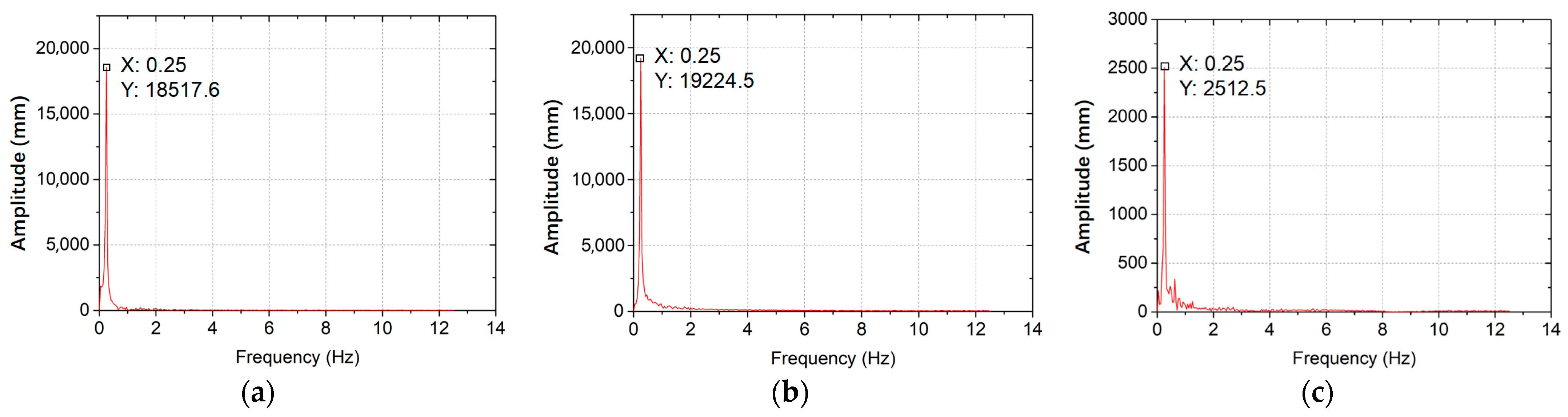
The motion of the blade was also analyzed in the frequency domain [51]. As an example, the 3D motion of P2 was studied with Fourier transform. In the corresponding frequency domain, only a fundamental frequency signal caused by rotation existed, as shown in Figure 15, indicating the wind turbine was in working order.
4. Discussion
For the self-calibration method, the distribution of control points is closely related to the calibration method. Insufficient control points or low matching accuracy may lead to the degradation of the calibration calculation model. Unfortunately, these factors that affect the calibration accuracy cannot be predicted before measurement. To solve this problem, we propose an extrinsic parameter self-calibration method. In this method, after the control points are chosen with the SURF algorithm, the mismatched control points are filtered out by implementing the image correlation algorithm. This procedure is critical in improving the accuracy and robustness of camera calibrations.
In addition, an innovative self-calibration method has been developed. After the control points are extracted, they are randomly divided into two groups. Two calibration methods, i.e., the epipolar-geometry-based and homography-based calibration methods, are employed in determining the extrinsic parameters using 90% of the control points. The resulting extrinsic parameters are examined with the remaining 10% of the control points. The re-projection error is used as a ruler to evaluate which calibration method excels in the competition. The framework potentially provides a way to select optimal calibration algorithms in test scenarios.
Camera motion often occurs in remote field measurements, which is one of the main sources of measurement error as an optical lever. Although mechanical equipment is helpful in reducing camera motion, errors caused by camera motion cannot be completely removed in 3D photogrammetry measurements. This study proposes a camera motion correction method based on BG points and motion model parameters. The proposed method avoids the repeated calibration of extrinsic parameters by correcting the motion of each camera separately. Note that the BG points selected in the two views are not necessarily the same because the motion parameters of the two cameras are completely independent.
Based on the analysis performed, the proposed method can serve as a reliable tool for the SHM of civil structures. However, since the measurement error caused by the illumination variation is not considered, the accuracy of the field measurement is still lower than that of a laboratory measurement. A recent study provided an algorithm that enables the real-time adjustment of the exposure of the camera [52], and the measurement accuracy was considerably improved in a mono-video deflectometer. This technique can be potentially helpful in a stereo-DIC system in outdoor applications. In addition, measurement errors caused by data loss, equipment dysfunction, light refraction, low visibility, etc., also need to be considered. In the future, we will continue to explore new techniques and methods to improve the performance of stereo vision for 3D displacement measurements of large structures.
5. Conclusions
This study presents a systematic study of stereo-DIC in field tests. A robust control point extraction procedure is elaborated. An adaptive extrinsic parameter self-calibration algorithm is developed to estimate the relative position and orientation of the stereo cameras. As high accuracy in the registration of control points is needed, the presented calibration method offers robust calibration with high accuracy. Furthermore, a reliable reference frame is established based on Euclidean transformation. A camera motion correction method based on BG points and motion model parameters is proposed.
A validation experiment was performed to evaluate the feasibility of the established stereo-DIC system and the proposed techniques. The technologies were also applied to evaluate a 2 MW wind turbine’s operation. The experimental results show that the proposed method is a convenient, contactless technique that enables the online, nondestructive evaluation of wind turbines in service without shutdown.
Author Contributions
Conceptualization, W.F. and D.Z.; methodology, W.F. and D.Z.; software, W.F.; validation, W.F., Q.L. and W.D.; formal analysis, W.F. and D.Z.; investigation, Q.L. and W.D.; resources, W.F.; writing—original draft preparation, W.F.; writing—review and editing, D.Z. and Q.L.; visualization, W.F. and W.D.; supervision, D.Z.; project administration, D.Z.; funding acquisition, D.Z., W.F. and Q.L. All authors have read and agreed to the published version of the manuscript.
Funding
This research was funded by A Project Supported by the Scientific Research Fund of the Zhejiang Provincial Education Department (Y202147608) and the Zhejiang Provincial Natural Science Foundation of China under Grant No. LTGG23E080008.
Data Availability Statement
Not applicable.
Conflicts of Interest
The authors declare no conflict of interest.
References
- Zhang, D.; Yu, Z.; Xu, Y.; Ding, L.; Ding, H.; Yu, Q.; Su, Z. GNSS aided long-range 3D displacement sensing for high-rise structures with two non-overlapping cameras. Remote Sens. 2022, 14, 379. [Google Scholar] [CrossRef]
- Luo, R.; Zhou, Z.; Chu, X.; Ma, W.; Meng, J. 3D deformation monitoring method for temporary structures based on multi-thread LiDAR point cloud. Measurement 2022, 200, 111545. [Google Scholar] [CrossRef]
- Shen, N.; Chen, L.; Liu, J.; Wang, L.; Tao, T.; Wu, D.; Chen, R. A review of global navigation satellite system (GNSS)-based dynamic monitoring technologies for structural health monitoring. Remote Sens. 2019, 11, 1001. [Google Scholar] [CrossRef] [Green Version]
- Dong, C.; Celik, O.; Catbas, F.N.; O’Brien, E.J.; Taylor, S.; Engineering, I. Structural displacement monitoring using deep learning-based full field optical flow methods. Struct. Infrastruct. Eng. 2020, 16, 51–71. [Google Scholar] [CrossRef]
- Entezami, A.; Arslan, A.N.; De Michele, C.; Behkamal, B. Online hybrid learning methods for real-time structural health monitoring using remote sensing and small displacement data. Remote Sens. 2022, 14, 3357. [Google Scholar] [CrossRef]
- Liu, G.; He, C.; Zou, C.; Wang, A. Displacement measurement based on UAV images using SURF-enhanced camera calibration algorithm. Remote Sens. 2022, 14, 6008. [Google Scholar] [CrossRef]
- Tian, L.; Ding, T.; Pan, B. Generalized scale factor calibration method for an off-axis digital image correlation-based video deflectometer. Sensors 2022, 22, 10010. [Google Scholar] [CrossRef]
- Wang, S.; Zhang, S.; Li, X.; Zou, Y.; Zhang, D. Development of monocular video deflectometer based on inclination sensors. Smart Struct. Syst. 2019, 25, 607–616. [Google Scholar]
- Luo, P.; Wang, L.; Li, D.; Yang, J.; Lv, X. Deformation and failure mechanism of horizontal soft and hard interlayered rock under uniaxial compression based on digital image correlation method. Eng. Fail. Anal. 2022, 142, 106823. [Google Scholar] [CrossRef]
- Bardakov, V.V.; Marchenkov, A.Y.; Poroykov, A.Y.; Machikhin, A.S.; Sharikova, M.O.; Meleshko, N.V. Feasibility of digital image correlation for fatigue cracks detection under dynamic loading. Sensors 2021, 21, 6457. [Google Scholar] [CrossRef]
- Garbowski, T.; Maier, G.; Novati, G. Diagnosis of concrete dams by flat-jack tests and inverse analyses based on proper orthogonal decomposition. J. Mech. Mater. Struct. 2011, 6, 181–202. [Google Scholar] [CrossRef] [Green Version]
- Gajewski, T.; Garbowski, T. Calibration of concrete parameters based on digital image correlation and inverse analysis. Arch. Civ. Mech. Eng. 2014, 14, 170–180. [Google Scholar] [CrossRef]
- Gajewski, T.; Garbowski, T. Mixed experimental/numerical methods applied for concrete parameters estimation. In Proceedings of the 20th International Conference on Computer Methods in Mechanics (CMM2013), Poznań, Poland, 27–31 August 2013; pp. 293–302. [Google Scholar]
- Chuda-Kowalska, M.; Gajewski, T.; Garbowski, T. Mechanical characterization of orthotropic elastic parameters of a foam by the mixed experimental-numerical analysis. J. Theor. App. Mech. 2015, 53, 383–394. [Google Scholar] [CrossRef] [Green Version]
- Garbowski, T.; Maier, G.; Novati, G. On calibration of orthotropic elastic-plastic constitutive models for paper foils by biaxial tests and inverse analyses. Struct. Multidiscip. Optim. 2012, 46, 111–128. [Google Scholar] [CrossRef] [Green Version]
- Garbowski, T.; Grabski, J.K.; Marek, A. Full-field measurements in the edge crush test of a corrugated board—Analytical and numerical predictive models. Materials 2021, 14, 2840. [Google Scholar] [CrossRef]
- Garbowski, T.; Knitter-Piątkowska, A.; Marek, A. New edge crush test configuration enhanced with full-field strain measurements. Materials 2021, 14, 5768. [Google Scholar] [CrossRef]
- Su, Z.; Lu, L.; Yang, F.; He, X.; Zhang, D. Geometry constrained correlation adjustment for stereo reconstruction in 3D optical deformation measurements. Opt. Express 2020, 28, 12219–12232. [Google Scholar] [CrossRef]
- Seo, S.; Ko, Y.; Chung, M. Evaluation of field applicability of high-Speed 3D digital image correlation for shock vibration measurement in underground mining. Remote Sens. 2022, 14, 3133. [Google Scholar] [CrossRef]
- Reu, P.L.; Toussaint, E.; Jones, E.; Bruck, H.A.; Iadicola, M.; Balcaen, R.; Simonsen, M. DIC challenge: Developing images and guidelines for evaluating accuracy and resolution of 2D analyses. Exp. Mech. 2018, 58, 1067–1099. [Google Scholar] [CrossRef]
- Xu, A.; Jiang, G.; Bai, Z. A practical extrinsic calibration method for joint depth and color sensors. Opt. Laser. Eng. 2022, 149, 106789. [Google Scholar] [CrossRef]
- Zhang, Z. A flexible new technique for camera calibration. IEEE Trans. Pattern Anal. Mach. Intell. 2000, 22, 1330–1334. [Google Scholar] [CrossRef] [Green Version]
- Xu, X.; Liu, M.; Peng, S.; Ma, Y.; Zhao, H.; Xu, A. An in-orbit stereo navigation camera self-calibration method for planetary rovers with multiple constraints. Remote Sens. 2022, 14, 402. [Google Scholar] [CrossRef]
- Beaubier, B.; Dufour, J.-E.; Hild, F.; Roux, S.; Lavernhe, S.; Lavernhe-Taillard, K. CAD-based calibration and shape measurement with stereoDIC. Exp. Mech. 2014, 54, 329–341. [Google Scholar] [CrossRef]
- An, Y.; Bell, T.; Li, B.; Xu, J.; Zhang, S. Method for large-range structured light system calibration. Appl. Opt. 2016, 55, 9563–9572. [Google Scholar] [CrossRef] [PubMed]
- Gao, Z.; Gao, Y.; Su, Y.; Liu, Y.; Fang, Z.; Wang, Y.; Zhang, Q. Stereo camera calibration for large field of view digital image correlation using zoom lens. Measurement 2021, 185, 109999. [Google Scholar] [CrossRef]
- Chen, B.; Genovese, K.; Pan, B. Calibrating large-FOV stereo digital image correlation system using phase targets and epipolar geometry. Opt. Laser. Eng. 2022, 150, 106854. [Google Scholar] [CrossRef]
- Liu, Z.; Li, F.; Li, X.; Zhang, G. A novel and accurate calibration method for cameras with large field of view using combined small targets. Measurement 2015, 64, 1–16. [Google Scholar] [CrossRef]
- Chen, B.; Pan, B. Camera calibration using synthetic random speckle pattern and digital image correlation. Opt. Laser. Eng. 2020, 126, 105919. [Google Scholar] [CrossRef]
- Zhong, F.; Indurkar, P.P.; Quan, C. Three-dimensional digital image correlation with improved efficiency and accuracy. Measurement 2018, 128, 23–33. [Google Scholar] [CrossRef]
- Chen, B.; Pan, B. Mirror-assisted multi-view digital image correlation: Principles, applications and implementations. Opt. Laser. Eng. 2022, 149, 106786. [Google Scholar] [CrossRef]
- Shi, B.; Liu, Z.; Zhang, G. Online stereo vision measurement based on correction of sensor structural parameters. Opt. Express 2021, 29, 37987–38000. [Google Scholar] [CrossRef] [PubMed]
- Yu, Q.; Guan, B.; Shang, Y.; Liu, X. Flexible camera series network for deformation measurement of large scale structures. Smart Struct. Syst. 2019, 24, 587–595. [Google Scholar]
- Jiao, J.; Guo, J.; Fujita, K.; Takewaki, I. Displacement measurement and nonlinear structural system identification: A vision-based approach with camera motion correction using planar structures. Struct. Control Health Monit. 2021, 28, e2761. [Google Scholar] [CrossRef]
- Lee, J.; Lee, K.-C.; Jeong, S.; Lee, Y.-J.; Sim, S.H. Long-term displacement measurement of full-scale bridges using camera ego-motion compensation. Mech. Syst. Signal Process. 2020, 140, 106651. [Google Scholar] [CrossRef]
- Chen, R.; Li, Z.; Zhong, K.; Liu, X.; Wu, Y.; Wang, C.; Shi, Y. A stereo-vision system for measuring the ram speed of steam hammers in an environment with a large field of view and strong vibrations. Sensors 2019, 19, 996. [Google Scholar] [CrossRef] [Green Version]
- Barros, F.; Sousa, P.J.; Tavares, P.J.; Moreira, P.M.J.P. Robust reference system for digital image correlation camera recalibration in fieldwork. Procedia Struct. Integr. 2018, 13, 1993–1998. [Google Scholar] [CrossRef]
- Chen, J.; Davis, A.; Wadhwa, N.; Durand, F.; Freeman, W.T.; Büyüköztürk, O. Video camera–based vibrations measurement for civil infrastructure applications. J. Infrastruct. Syst. 2017, 23, B4016013. [Google Scholar] [CrossRef]
- Abolhasannejad, V.; Huang, X.; Namazi, N. Developing an optical image-based method for bridge deformation measurement considering camera motion. Sensors 2018, 18, 2754. [Google Scholar] [CrossRef] [Green Version]
- Yoon, H.; Shin, J.; Spencer, B.F., Jr. Structural displacement measurement using an unmanned aerial system. Comput.-Aided Civ. Inf. 2018, 33, 183–192. [Google Scholar] [CrossRef]
- Yin, Y.; Zhu, H.; Yang, P.; Yang, Z.; Liu, K.; Fu, H. Robust and accuracy calibration method for a binocular camera using a coding planar target. Opt. Express 2022, 30, 6107–6128. [Google Scholar] [CrossRef]
- Zisserman, R.H.A. Multiple View Geometry in Computer Vision; Cambridge University Press: Cambridge, UK, 2003; pp. 239–259. [Google Scholar]
- Pastucha, E.; Puniach, E.; Ścisłowicz, A.; Ćwiąkała, P.; Niewiem, W.; Wiącek, P. 3D reconstruction of power lines using uav images to monitor corridor clearance. Remote Sens. 2020, 12, 3698. [Google Scholar] [CrossRef]
- Bansal, M.; Kumar, M.; Kumar, M. 2D object recognition: A comparative analysis of SIFT, SURF and ORB feature descriptors. Multimed. Tools Appl. 2021, 80, 18839–18857. [Google Scholar] [CrossRef]
- Ye, X.; Zhao, J. A novel rotated sigmoid weight function for higher performance in heterogeneous deformation measurement with digital image correlation. Opt. Laser. Eng. 2022, 159, 107214. [Google Scholar] [CrossRef]
- Pan, B. An evaluation of convergence criteria for digital image correlation using inverse compositional Gauss–Newton algorithm. Strain 2014, 50, 48–56. [Google Scholar] [CrossRef]
- Hartley, R.I. In defense of the eight-point algorithm. IEEE Trans. Pattern Anal. Mach. Intell. 1997, 19, 580–593. [Google Scholar] [CrossRef] [Green Version]
- Ping, Y.; Liu, Y. A calibration method for line-structured light system by using sinusoidal fringes and homography matrix. Optik 2022, 261, 169192. [Google Scholar] [CrossRef]
- Zhao, K.; Han, Q.; Zhang, C.; Xu, J.; Cheng, M. Deep Hough transform for semantic line detection. IEEE Trans. Pattern Anal. Mach. Intell. 2022, 44, 4793–4806. [Google Scholar] [CrossRef]
- Min, C.; Gu, Y.; Li, Y.; Yang, F. Non-rigid infrared and visible image registration by enhanced affine transformation. Pattern Recogn. 2020, 106, 107377. [Google Scholar] [CrossRef]
- Wu, R.; Zhang, D.; Yu, Q.; Jiang, Y.; Arola, D. Health monitoring of wind turbine blades in operation using three-dimensional digital image correlation. Mech. Syst. Signal Process. 2019, 130, 470–483. [Google Scholar] [CrossRef]
- Yang, D.; Zhang, S.; Wang, S.; Yu, Q.; Su, Z.; Zhang, D. Real-time illumination adjustment for video deflectometers. Struct. Control Health Monit. 2022, 29, e2930. [Google Scholar] [CrossRef]
Figure 1.
Flowchart of the proposed methods.
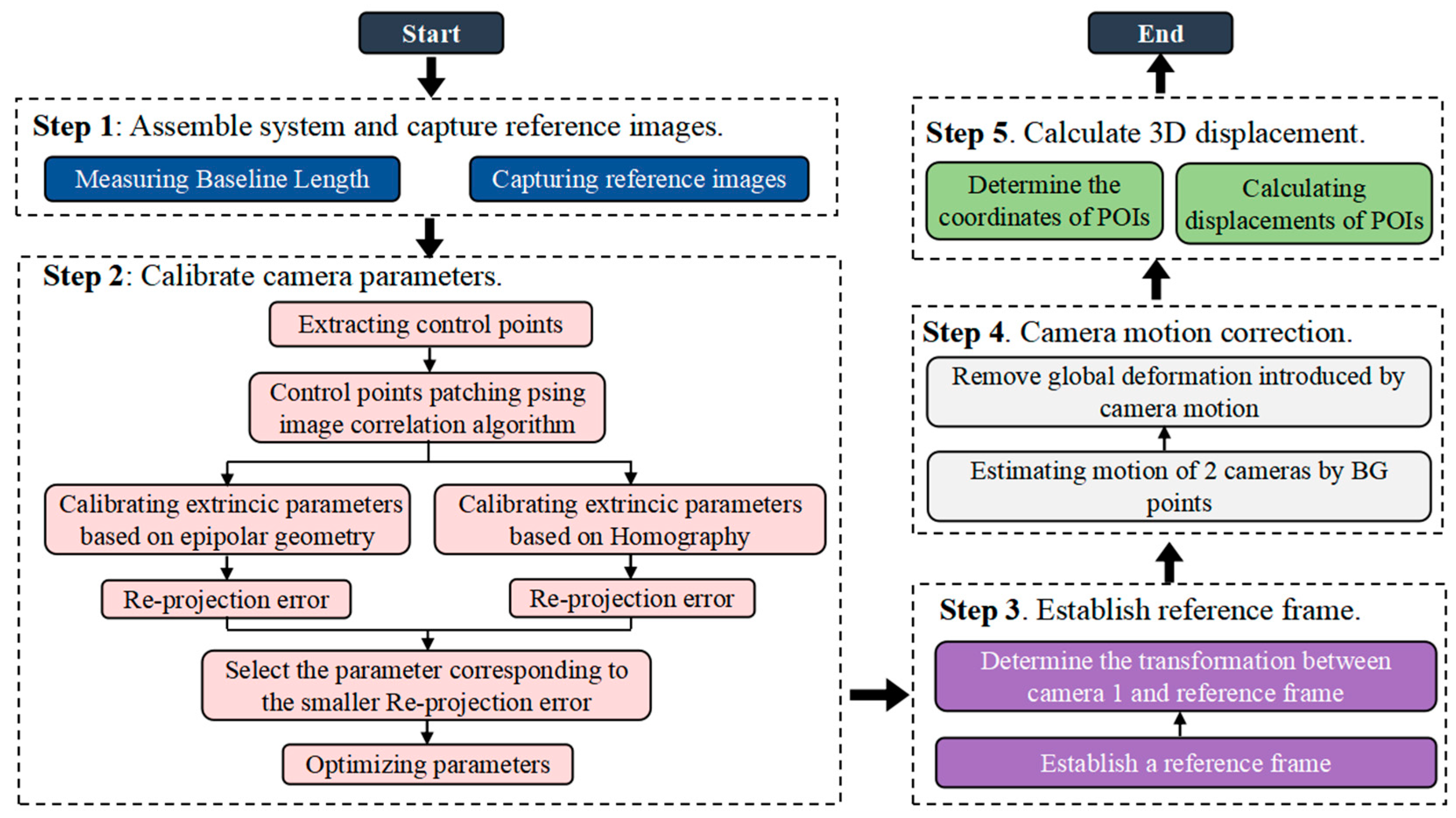
Figure 2.
Triangular regulation: (a) epipolar constraint; (b) homography constraint.

Figure 3.
Schematic principle of control point matching based on an image correlation algorithm.
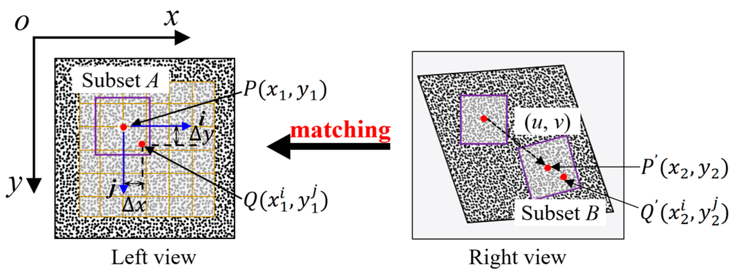
Figure 4.
Schematic principle of establishing reference frame.
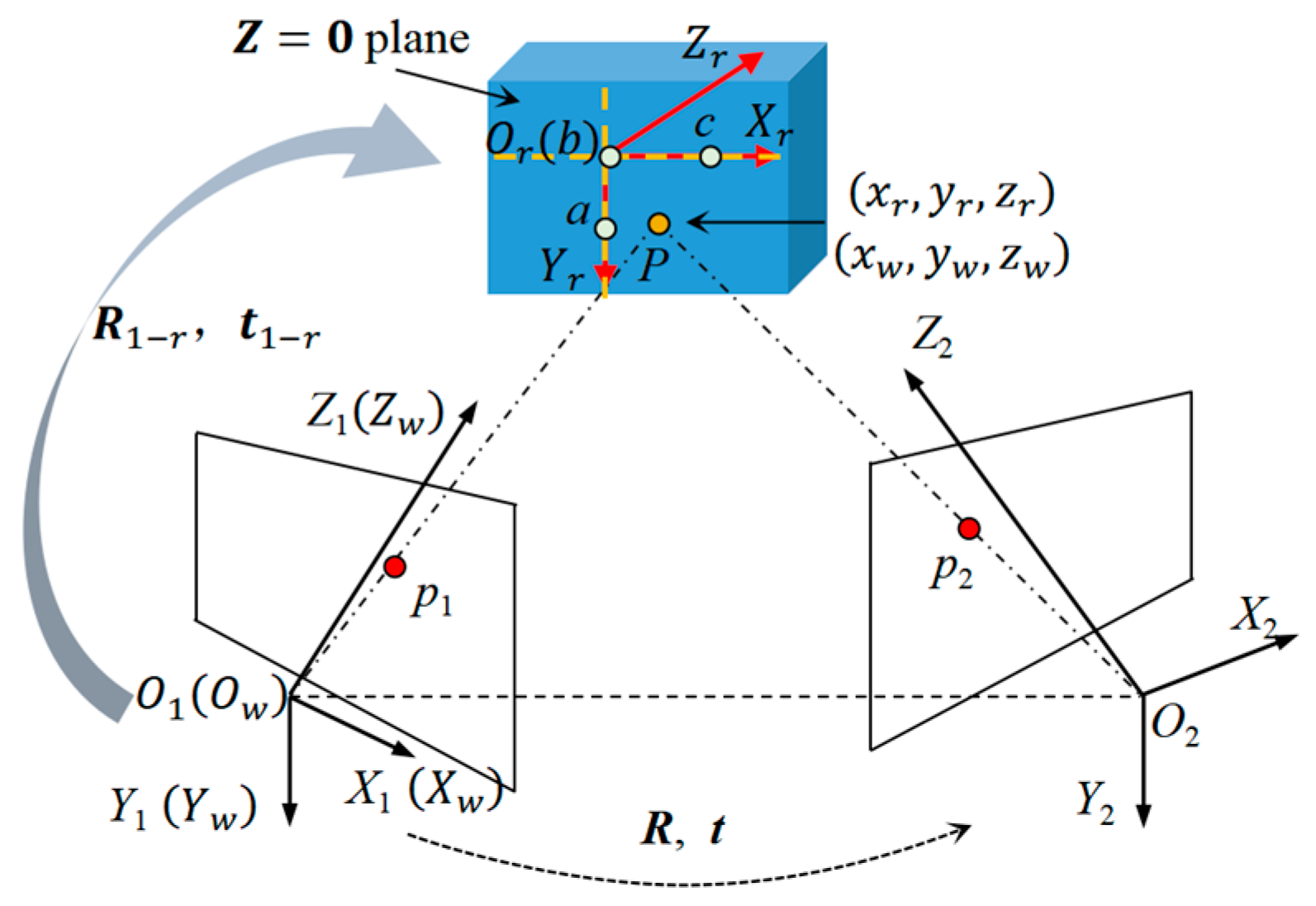
Figure 5.
Coordinate localization of POIs: (a) POIs in the left view; (b) localization based on epipolar constraints; (c) localization based on homography constraints.
Figure 5.
Coordinate localization of POIs: (a) POIs in the left view; (b) localization based on epipolar constraints; (c) localization based on homography constraints.
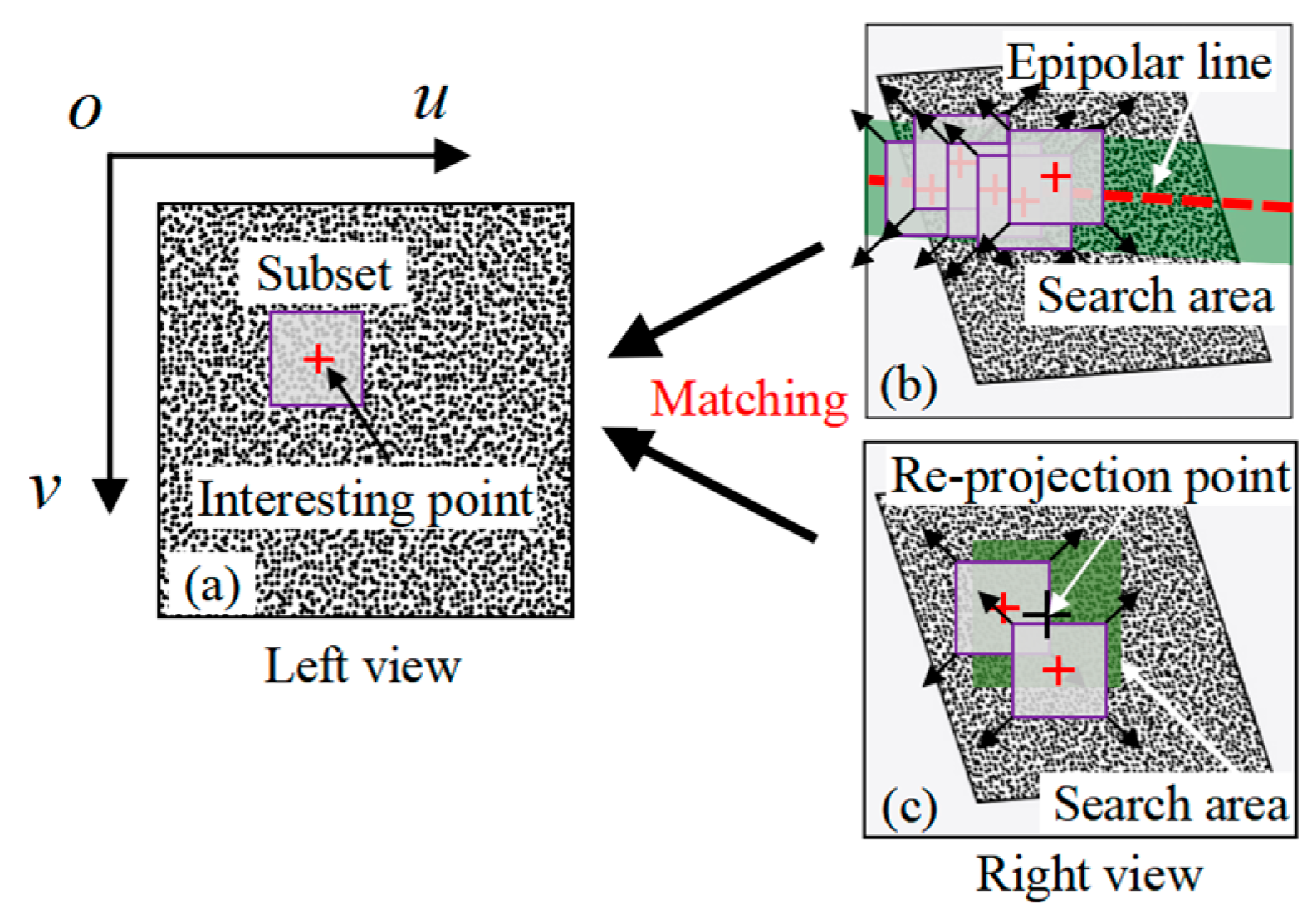
Figure 6.
Stereo-DIC system for field applications: (a) schematic diagram; (b) measurement station configuration.
Figure 6.
Stereo-DIC system for field applications: (a) schematic diagram; (b) measurement station configuration.

Figure 7.
Experimental setup: (a) satellite view of the experimental location; (b) layout of the experimental site.
Figure 7.
Experimental setup: (a) satellite view of the experimental location; (b) layout of the experimental site.
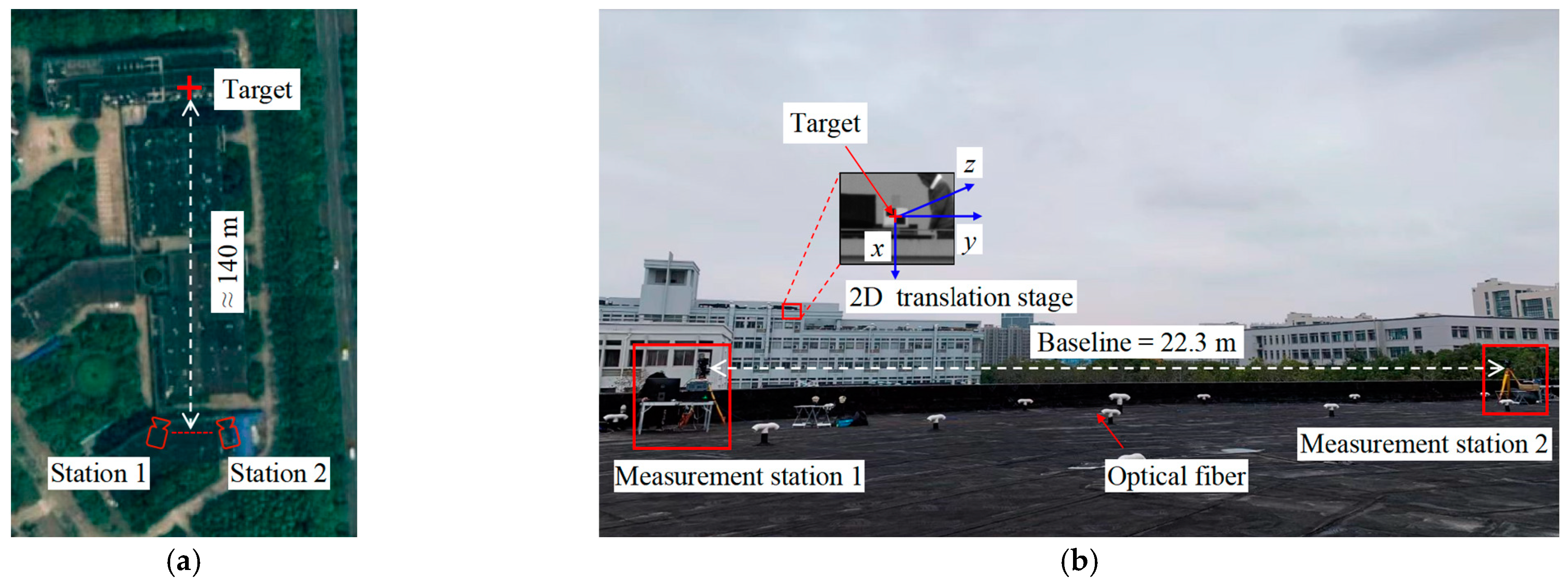
Figure 8.
Control point matching: (a) reference image with mismatches; (b) reference image after deleting mismatches.
Figure 8.
Control point matching: (a) reference image with mismatches; (b) reference image after deleting mismatches.

Figure 9.
The reference frame and BG points: (a) left view; (b) right view.
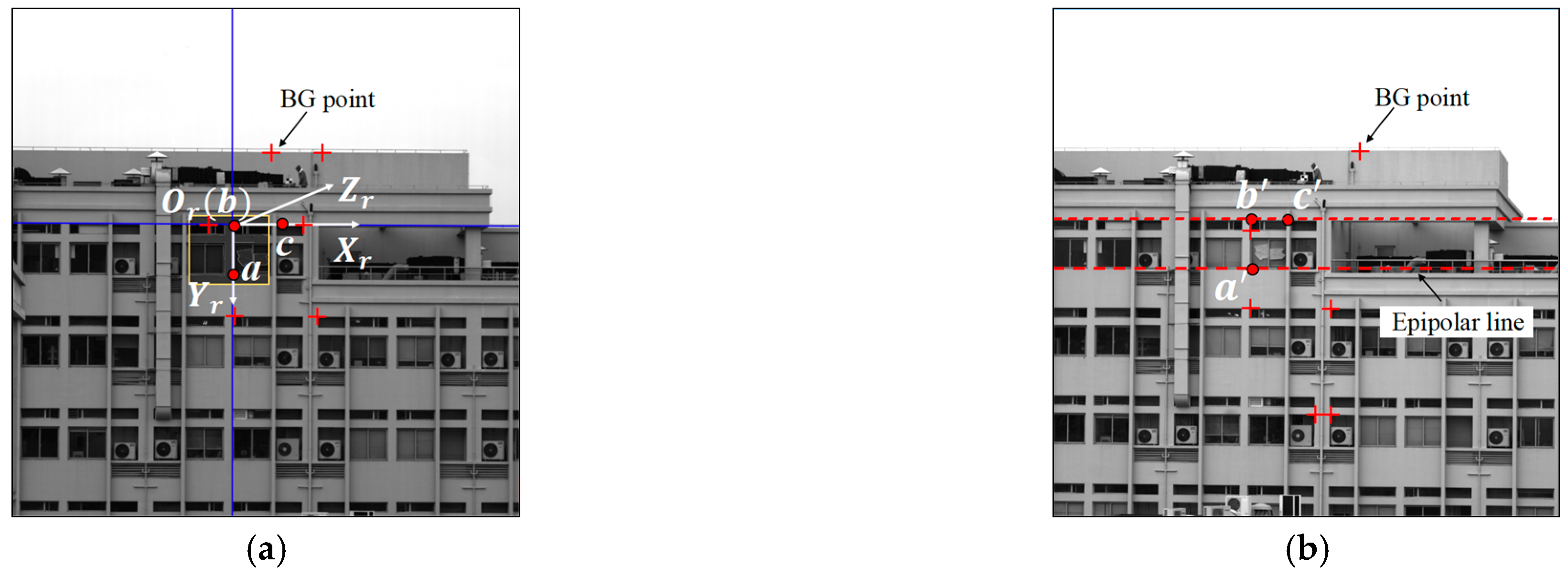
Figure 10.
Three−dimensional displacements of the target before and after camera motion correction: (a) x−direction; (b) y−direction; (c) z−direction.
Figure 10.
Three−dimensional displacements of the target before and after camera motion correction: (a) x−direction; (b) y−direction; (c) z−direction.
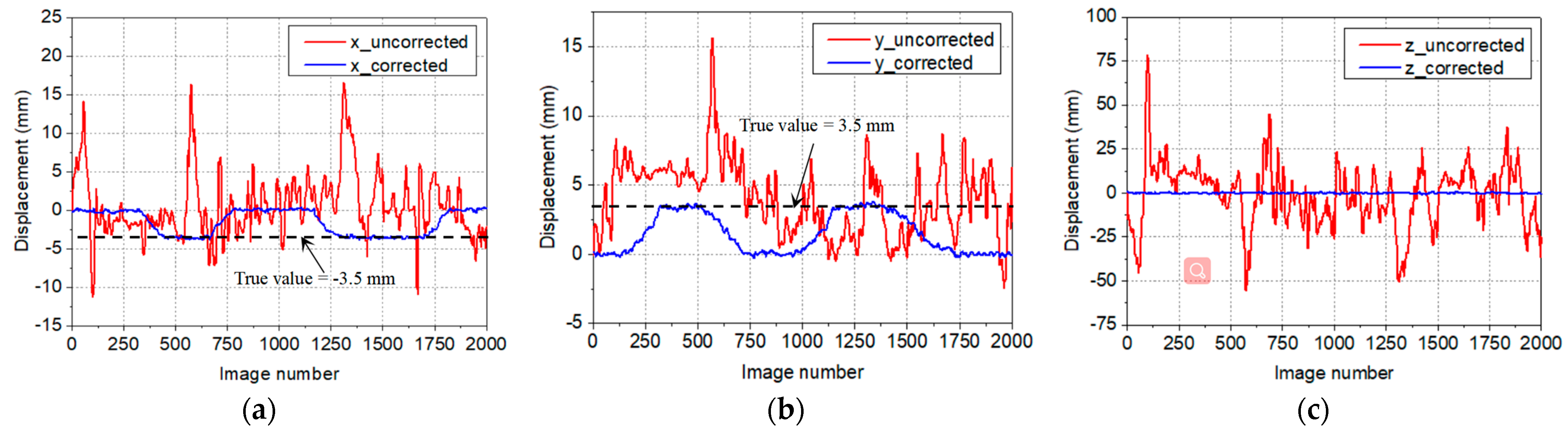
Figure 11.
Random speckle patterns on the pressure side of the wind turbine blades.
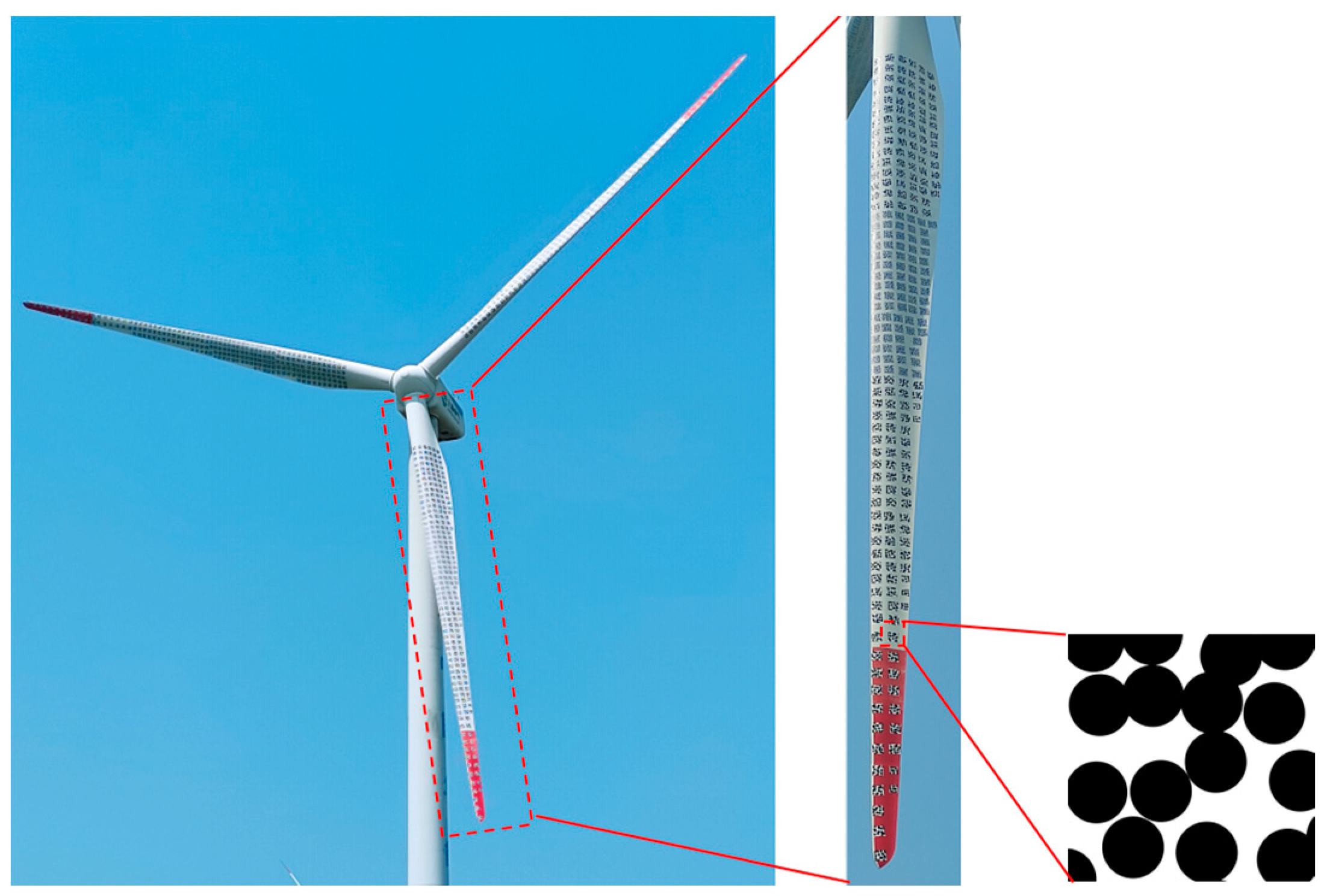
Figure 12.
Experimental setup: (a) arrangement of the measurement stations around the wind turbine; (b) a measurement station.
Figure 12.
Experimental setup: (a) arrangement of the measurement stations around the wind turbine; (b) a measurement station.
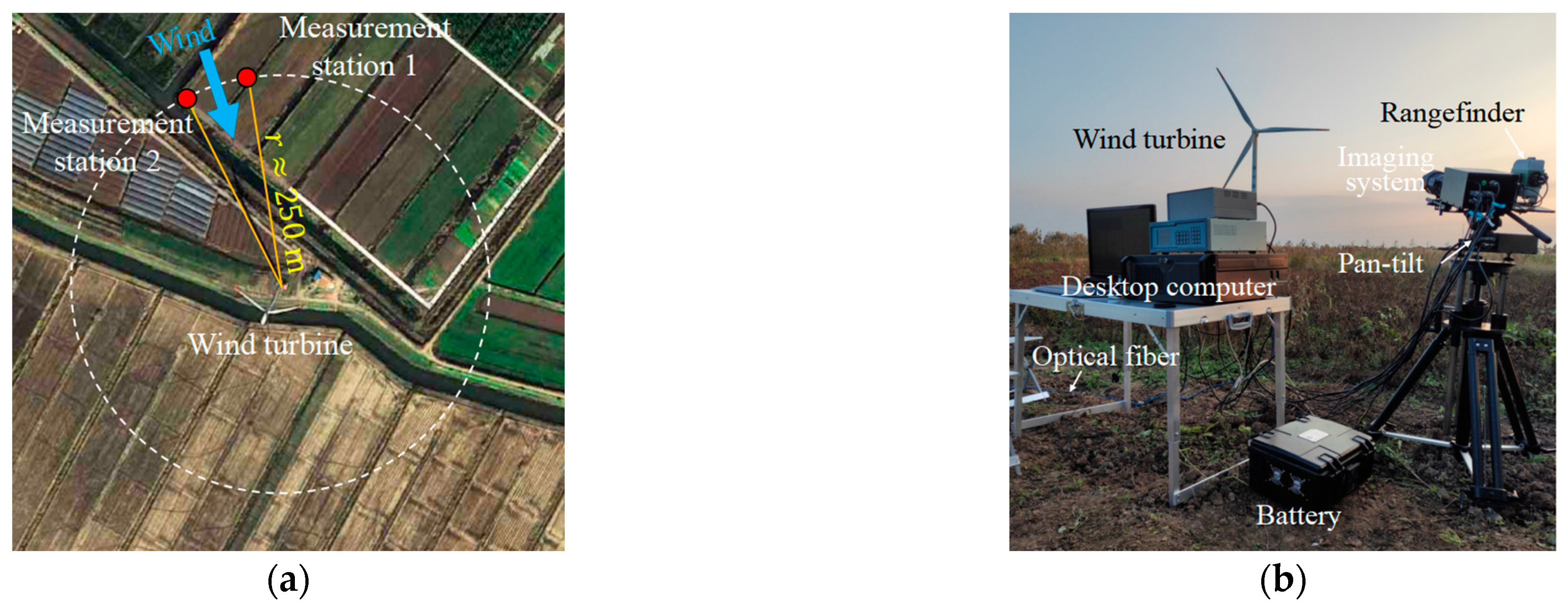
Figure 13.
Control points and POIs of wind turbine blades: (a) control points; (b) points of interest.
Figure 13.
Control points and POIs of wind turbine blades: (a) control points; (b) points of interest.

Figure 14.
Three−dimensional movement of the POIs: (a) P1; (b) P2; (c) P3.
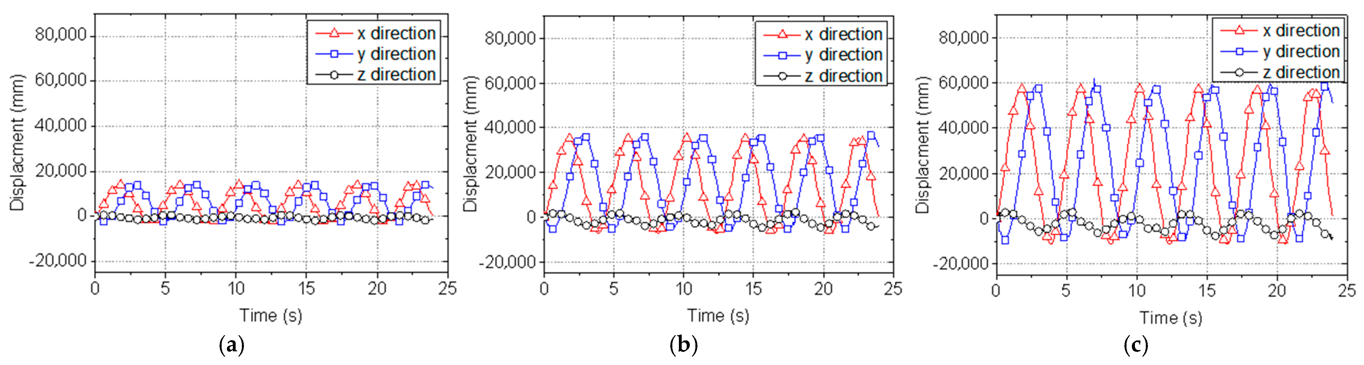
Figure 15.
Frequency spectrum the 3D motion of P2: (a) x−direction; (b) y−direction; (c) z−direction.
Figure 15.
Frequency spectrum the 3D motion of P2: (a) x−direction; (b) y−direction; (c) z−direction.

Table 1.
The parameters of the stereo-DIC system and re-projection errors.
| Intrinsic Parameters | /Pixels | /Pixels | ||
|---|---|---|---|---|
| Camera 1 | (1261.06, 1275.54) | (15,911.12, 16,069.63) | (0.56, −31.27) | |
| Camera 2 | (1258.26, 1279.05) | (15,870.17, 16,088.24) | (0.38, 15.62) | |
| Extrinsic Parameters | Method | Rotation Vector (°) | Translation Vector (mm) | Error (pixels) |
| Epipolar geometry-based | () | (22,041.47, −186.96, 7551.71) | 0.21 | |
| Homography-based | (0.14, 8.32, −0.64) | (22,035.01, −115.29, 7573.09) | 0.47 |
Table 2.
Relative rotation and translation vectors between camera 1 and the reference frame.
| Rotation Angle (°) | Translation Vector (mm) |
|---|---|
| (0.25, 7.54, 0.19) | (−19,286.21, −987.17, 135,041.34) |
Table 3.
The parameters of the stereo-DIC system and re-projection errors.
| Intrinsic Parameters | /Pixels | /Pixels | ||
|---|---|---|---|---|
| Camera 1 | (2194.99, 2374.92) | (16,716.56, 16,554.44) | (−0.06, 4.58) | |
| Camera 2 | (2175.87, 2474.15) | (16,195.47, 16,036.88) | (−0.01, −2.41) | |
| Extrinsic Parameters | Rotation Vector (°) | Translation Vector (mm) | Error (pixels) | |
| (−0.24, 14.19, −2.97) | (63,252.85, 2414.49, 8747.62) | 0.15 | ||
Disclaimer/Publisher’s Note: The statements, opinions and data contained in all publications are solely those of the individual author(s) and contributor(s) and not of MDPI and/or the editor(s). MDPI and/or the editor(s) disclaim responsibility for any injury to people or property resulting from any ideas, methods, instructions or products referred to in the content. |
© 2023 by the authors. Licensee MDPI, Basel, Switzerland. This article is an open access article distributed under the terms and conditions of the Creative Commons Attribution (CC BY) license (https://creativecommons.org/licenses/by/4.0/).
Share and Cite
MDPI and ACS Style
Feng, W.; Li, Q.; Du, W.; Zhang, D. Remote 3D Displacement Sensing for Large Structures with Stereo Digital Image Correlation. Remote Sens. 2023, 15, 1591. https://doi.org/10.3390/rs15061591
AMA Style
Feng W, Li Q, Du W, Zhang D. Remote 3D Displacement Sensing for Large Structures with Stereo Digital Image Correlation. Remote Sensing. 2023; 15(6):1591. https://doi.org/10.3390/rs15061591
Chicago/Turabian StyleFeng, Weiwu, Qiang Li, Wenxue Du, and Dongsheng Zhang. 2023. "Remote 3D Displacement Sensing for Large Structures with Stereo Digital Image Correlation" Remote Sensing 15, no. 6: 1591. https://doi.org/10.3390/rs15061591
Note that from the first issue of 2016, this journal uses article numbers instead of page numbers. See further details here.