Article

Flood Monitoring Using Satellite-Based RGB Composite Imagery and Refractive Index Retrieval in Visible and Near-Infrared Bands

Department of Environment, Energy and Geoinfomatics, Sejong University, Seoul 05006, Korea
*
Author to whom correspondence should be addressed.
Remote Sens. 2017, 9(4), 313; https://doi.org/10.3390/rs9040313
Submission received: 24 November 2016 / Revised: 7 March 2017 / Accepted: 24 March 2017 / Published: 27 March 2017

Abstract

:
Satellite remote sensing provides significant information for the monitoring of natural disasters. Recently, on a global scale, floods have been increasing both in frequency and in magnitude. In order to map the inundation area, flooding events are investigated using unique RGB composite imagery based on the MODIS surface reflectance (MOD09GA) data obtained from the Terra satellite, which is used to visualize and analyze these events. This study proposes using an RGB combination of MODIS band 6 (1.64 μm), band 5 (1.24 μm), and band 2 (0.86 μm) data from the visible and the near-infrared spectral ranges to map flood events. The flooding events that were investigated in this study occurred on 25 October 2015 along the Pampanga River in the Philippines, and on 28 July 2016 along the Poyang and Dongting Lakes in China. In the case of the Pampanga River, the inundated areas were estimated with surface reflectance (R) thresholds of 0.0 ≤ R6 ≤ 0.102, 0.0 ≤ R5 ≤ 0.138, and 0.03 ≤ R2 ≤ 0.148 for MODIS bands 6, 5, and 2, respectively, which were determined using Otsu’s method. The total inundated area was estimated to be 487.75 km2. This estimate was indirectly compared with the results obtained from SENTINEL-1A Synthetic Aperture Radar (SAR) data. The total inundated area on 26 October 2015 for the case of the Pampanga River was estimated to be 486.37 km2 using histogram analysis based on Otsu’s method. For the flooding case in China, the total estimated inundated area using MODIS RGB imagery on 28 July 2016 and SAR on 3 August 2016 was 1148.25 km2 and 1110.096 km2, respectively. In addition, RGB imagery results using MODIS 6-5-2 bands were supported by the refractive index retrieval along the inundation area. A threshold of 1.6 for the real part of the complex refractive index allows for the discrimination between the flooded and non-flooded areas using the Hong and ASH approximations. This study shows that the RGB composite techniques using advanced sensors with more bands and higher spatio-temporal resolutions, and supported by the refractive index retrieval method, are useful for estimating flood events.

1. Introduction

The recent increase in the number of natural disasters has become a global issue, because of the damages to the hydrological and ecological environment and human-made infrastructure, and the threats to human lives. Satellite remote sensing techniques provide valuable support for monitoring these disasters and for post-event crisis management.
To obtain detailed and valuable information for flood monitoring, satellite missions, such as TerraSAR-X, Radarsat-2, and the Cosmo-SkyMed constellation, with Synthetic Aperture Radar (SAR) data, have been used to support flood emergency situations [1,2,3,4,5,6]. Many studies have demonstrated the effectiveness of SAR data in mapping wetlands [7,8], because it has the advantage of observations during the night and day, and under cloud cover [9,10]. However, these methods also have a disadvantage: SAR data largely depends on the accuracy of the determined thresholds that are usually static in space and time, despite the significant variability of the backscatter. This may lead to the misidentification of pixels [11].
Despite the limitations of optical satellites, which are mainly due to the effects of cloud cover, a flood detection method using visible (VIS) and near-infrared (NIR) bands was investigated [12]. One of the benefits of using these satellites is the ability to visualize flooded areas, separately, without including the non-flooded areas. Much of the pioneering work on the remote sensing of floods using band 0.8–1.1 μm of Landsat-1 [13,14,15,16,17,18] was accomplished for flooding in Iowa [19,20], Arizona [21], Virginia [20], and along the Mississippi River [22,23,24]. The Advanced Very High Resolution Radiometer (AVHRR) has also been successfully used for studying very large river floods [25,26,27,28], displaying three-band color composites for visual analysis, because flood and standing water absorbs infrared wavelengths of energy and appears as blue or black in the RGB composite imagery [29]. Flood monitoring based on the land surface temperature and Normalized Difference Vegetation Index (NDVI) [30,31] is also studied, because the NDVI tends to have a positive value in an area containing a dense vegetation canopy, and is low for standing water in both VIS and IR spectral bands. The normalized difference water index (NDWI) generally serves to distinguish water areas from non-water areas. It typically uses the difference between green and near-infrared bands [32]. Various studies have applied this method using other wavelength bands, such as short-wave infrared (SWIR) and mid-infrared (MIR) bands [33,34]. However, NDWI is sometimes ineffective in extracting water features in the case of urban areas, because the reflectance pattern of urban features is similar to that of water in the green band [35]. To compensate for this weakness, Xu suggested a new NDWI method (modified NDWI) that uses green and MIR bands [36]. Many of the studies for flood detection in non-water areas have applied both NDWI and modified NDWI to generate inundation hazard models and maps, and to calculate the flooded areas [35,37,38]. The Moderate Resolution Imaging Spectrometer (MODIS) onboard the Aqua and Terra satellites [39,40] is a useful instrument for mapping inundation areas, regardless of the optical sensors’ major disadvantage related to cloud cover. Different techniques for the use of MODIS data have been discussed, considering both their advantages and drawbacks [41,42,43]. These techniques usually have high frequency temporal measurements as far as the inundation extent is concerned. However, they are not ideal for detecting the flooded area on a fine scale, due to their low spatial resolution, which ranges from 250 m to 1 km. Despite these limitations, various approaches that use the MODIS data, such as spectral indices, have been employed to prevent the hazards of a flooding event [44,45,46].
The reflectance of terrestrial surfaces is often characterized mathematically, by the bidirectional reflectance distribution function (BRDF), which depends on the incident and reflected viewing directions, and the refractive index ( n ^ = n + i · k ,   i = 1 ) of the surface itself. In the VIS and NIR spectral regions, the vertical profiles of the soil moisture, temperature, and organic matter, are not significant for modeling [47]. Accordingly, red-green-blue (RGB) composite imagery based on the surface reflectances are useful because, physically, the surface reflection like absorption, transmission, emission, and scattering, requires a priori knowledge of the complex refractive index of a medium [48,49].
In this study, we provide a new RGB-composite technique that combines appropriate bands for mapping the inundation area based on knowledge of spectral bands and empirical experience. We investigated the flooding of the Pampanga River in the Philippines (Figure 1a), and the Poyang and Dongting Lakes in China (Figure 1b). In the case of the Pampanga River, a riverside flooding event occurred on 25 October 2015 due to Typhoon Koppu. Figure 2 shows the true color images of the Pampanga River area on 16 September 2015 at 02:20 UTC in the pre-flooding stage, and on 25 October 2015 at 02:25 UTC in the post-flooding stage. The case of the Poyang and Dongting Lakes occurred due to the heavy rainfall during the monsoon season and Typhoon Chaba. Figure 2c,d show the true color images using the surface reflectance values of the MODIS 1-4-3 bands , obtained on 27 March and 28 July 2016, respectively. We physically validated the proposed method for flood estimations using the refractive index retrieval derived by the Hong (Equation (6)) and ASH (Equation (8)) approximations using MODIS data, SENTINEL-1A Synthetic Aperture Radar (SAR) data for the same events.

2. Data and Methods

2.1. Data and Procedure

The MODIS instruments, which were onboard the TERRA launched in 1999, have 36 spectral bands ranging from 0.4 μm to 14.4 μm [50,51]. The nadir spatial resolution of bands 1 to 2, 3 to 7, and 8 to 36, are 250 m, 500 m, and 1 km, respectively. The MODIS surface reflectance data at 500 m resolution (MOD09GA) are used for masking the cloud and sea area. MOD09GA consists of seven bands in the VIS and NIR ranges, and we describe the information of each band as follows; MODIS band 1 (0.65 μm) corresponds to red light. Accordingly, the absorption of red lights in vegetation at this band results in being able to distinguish between vegetation and soil. Band 2 (0.86 μm), with strong absorption by water, is useful for separating water from dry soil or vegetated surfaces. Consequently, water appears dark, while soil and vegetation appear bright [52]. Band 3 (0.47 μm), corresponding to blue light, is useful for monitoring sediment in water and the water depth. Band 4 (0.56 μm) matches the wavelength of the green for vegetation. The sensitivity to moisture at Band 5 (1.24 μm), 6 (1.64 μm), and 7 (2.13 μm) are useful for monitoring the soil moisture and vegetation, and to differentiate the cloud and snow. The reflectance information of clay, sand, grass, snow, and water are shown with the MODIS spectral response function in Figure 3.
SAR data has frequently been used for flood detection due to its high resolution, minimal distortion from clouds, and guaranteed observations regardless of it being day or night [4]. However, SAR has a long observation period and is mainly used for historical analysis. One of the C-band SAR satellites, SENTINEL-1A, was launched in 2014 by the European Space Agency (ESA). We used Level-1, Ground Range Detected (GRD) data from SENTINEL-1A [54]. For SAR data, pre-processing was carried out to convert the intensity to a backscattering coefficient ( σ 0 ), and the Lee filter (7 × 7) method was applied to reduce the noise. Figure 4a,b show the VV(vertical transmitting, vertical receiving)-polarized backscattering coefficients ( σ 0 ) observed from SENTINEL-1A around the Pampanga River in the Philippines on 26 October 2015 at 21:46 UTC and around the Poyang and Dongting Lakes in China on 3 August 2016 at 10:27 UTC, respectively.
The research procedure (referred to in Figure 5) adopted in this study can be summarized as follows.
First, the surface reflectance values for VIS and NIR radiation were downloaded from the MODIS surface reflectance. Second, the separation of the flooded areas from the non-flooded areas was performed based on the distribution and threshold values of the surface reflectivity estimated using Otsu’s method, which is a simple and effective method for determining the threshold values, in order to extract objects from their background using binarization for the distribution of the histogram. The goodness of these thresholds was evaluated by measuring the separability of the gray-level classes [55]. Third, the three MODIS bands best suited to flooding detection were selected. Fourth, one-to-one matching of surface reflectivity values in the selected bands and RGB color saturations was performed. Finally, the flooded area in the RGB composite image was visualized and analyzed. The flooded area was indirectly compared using results obtained from the SENTINEL-1A SAR sensor. In addition, the model was physically validated using decomposed surface reflectivities and refractive indexes estimated from decomposed surface reflectivities.

2.2. RGB Composite Technique

The physical basis of the RGB color model is the tri-chromatic theory, in which three separate lights (red, green, and blue) can match any visible band [56]. The RGB space may be visualized as a cube with three axes corresponding to red, green, and blue. In the RGB space, according to Grassman’s first law of color mixture, a color can be matched by units of red, green, and blue in an n-bit display system, as follows [57]:
C i , j , k = R c ( r i ) + G c ( g j ) + B c ( b k ) ,   0 i , j , k < 2 n
where R C , G C , and B C are the units measured in any form that quantifies light power, C i , j , k is the color, and r i , g j , and b k represent the color saturation in red, green, and blue colors, respectively. The subscripts i , j , and k are the different contributions of RGB color saturation from 0 to 2 n , respectively.
In this study, the 8-bit computing colors are applied and n = 8 . In 8-bit computing, the color can range from 0 to 255 ( = 2 8 ). Accordingly, yellow (255, 255, 0), cyan (255, 0, 255), and magenta (0, 255, 255) can be analyzed as secondary colors, because the mixture of three-band observations determines an RGB color. Meanwhile, black (0, 0, 0) indicates no contribution and gray indicates an equal contribution from the three channels [57].
In this study, the key idea of RGB imaging is the one to one mapping of the satellite-observed surface reflectance ( R ) to a three-dimensional RGB color cube. The appropriate selection of Robservation bands in satellite sensors plays a key role in RGB image analysis. This combination requires knowledge of spectral bands and empirical experience of band combinations. Therefore, the color saturations in each of the red, green, and blue RGB colors can be rewritten as a function of R , within a range of maximum and minimum values of R at bands 1, 2, and 3 of the sensor onboard the satellite, as follows:
r i = 255 R i R i , M I N R i , M A X R i , M i I N ,   at   b a n d   i
g j = 255 R j R j , M I N R j , M A X R j , M I N ,   at   b a n d   j
b k = 255 R k R k , M I N R k , M A X R k , M I N ,   at   b a n d   k
where R i , R j , and R k are the surface reflectivities observed at bands i , j , and k of the MODIS sensor in this study, respectively.
In general, the gamma corrections for an image in 8-bit computing can be expressed as follows:
C o l o r   s a t u r a t i o n   =   255 [ R R M I N R M A X R M I I N ] 1 Γ
where Equations (2)–(4) are the specific form of gamma corrections with Γ = 1 to the color saturation. In this study, we use Γ = 1 .

2.3. Refractive Index Retrieval

Consequently, the RGB imagery depends on the appropriate selection and combination of observing bands, based on the knowledge of spectral bands and empirical experiences. To estimate the refractive index, many free-space experimental systems have been developed using the polarization ratio R H / R V [58,59]. Recently, R H / R V on a specular surface as a function of one polarization R V or R H , was derived from the generalized Fresnel equations [60], by taking the first term in the Taylor series of the logarithmic ratio ln R H / ln R V at the incidence angle θ [61], as follows:
R H R V = R V tan 2 θ
where RV and RH are polarized reflectances. The usefulness of Equation (6) was shown in a variety of applications, including in the detection of Asian dust (Hwangsa) [62], the validation of an IR sea-surface emissivity model [63], surface roughness retrieval [64,65], the estimation of global soil moisture [66], sea ice studies [67,68], and wind speed retrieval [69,70,71].
Recently, a squared form of Azzam’s relationship ( r ^ H = r ^ V · ( r ^ V c o s 2 θ ) / ( 1 r ^ V · c o s 2 θ ) ) [72,73,74] has been derived, as follows [75]:
R H R V = ( R V cos 2 θ ) 2 + 2 ( R V Re ( r ^ V ) cos 2 θ ) ( 1 R V cos 2 θ ) 2 + 2 ( R V Re ( r ^ V ) cos 2 θ )
where r ^ V = R e ( r ^ V ) + i · Im ( r ^ V ) , Re( r ^ V ) and Im( r ^ V ) are the real and imaginary part of r ^ V , respectively. R V = | r ^ V | 2 , and R H = | r ^ H | 2 .
Equation (7) requires a priori knowledge of the refractive index value because of the term of r ^ V , which is a complex value. However, for a non-absorbing material (k = 0), a squared form of Azzam’s relationship (Equation (7)) is simplified to an ASH approximation, as follows [75]:
R H R V = ( R V + cos 2 θ 1 + R V cos 2 θ ) 2
A method which can be used to estimate the refractive index based on the decomposition of unpolarized surface reflectivity [76] was presented using Equation (6) and no preference for either polarization [77], as follows:
R = R V + R H 2
where R V and R H can be numerically determined using Equations (6) or (8), and (9) for a given angle and a measured reflectivity.
The following solution is used to determine the refractive index from polarized reflectivities [78], along with a variety of inversion methods such as spectroscopic ellipsometry [79,80] and Kramers-Kronig phase shift analysis [81,82]:
n = B 2 A 2 + sin 2 θ + ( A 2 + B 2 sin 2 θ ) 2 + ( 2 A B ) 2 2   and   k = A B n ,
where B = ( a b ) sin θ cot 2 θ a b + ( 1 a 2 ) cos 2 θ 1 , A = B 2 2 a B cos θ cos 2 θ , a = R V + 1 R V 1 , and b = R H + 1 R H 1 . The refractive index of soil ranges from 1.39 + 0.0053i to 1.42 + 0.05i [83] in the optical band from 0.5 μm to 1.1 μm. The refractive index of water ranges from 1.339 + 1.86 × 10⁻⁹ i at 0.4 μm, to 1.296 + 2.89 × 10⁻⁹ i at 2.2 μm [81].

3. Results and Discussion

3.1. RGB Composite Technique

We tested an RGB combination of bands 1, 2, 3, 4, 5, 6, and 7 because of the spectral sensitivity, in order to distinguish water from soil/vegetation. This particular combination delineates the inundated and adjacent areas with a color contrast. We assume that the land surface is quasi-specular for computational efficiency, but the land surface is simulated as a linear combination of three Bidirectional Reflectance Distribution Function (BRDF) kernels [84]. Physically, the reflectance from a specular surface is larger than from a rough surface. The structure of the soil-water mixed layer is neglected and all of the constituents are regarded as evenly distributed. For monitoring floods, the distributions of reflectance at each band were described using the histograms in Figure 6. True color images of the Pampanga River make it easy to distinguish flooded and non-flooded areas (Figure 2). Bimodal distributions of the surface reflectance histograms were more suitable for the separation of the flooded areas from the non-flooded areas for MODIS band 2 (0.86 μm), band 5 (1.24 μm), and band 6 (1.64 μm) data. Thus, in the case of the Pampanga River, threshold values from Otsu’s method were determined as 0.0 ≤ R 6 ≤ 0.102, 0.0 ≤ R 5 ≤ 0.138, and 0.03 ≤ R 2 ≤ 0.148 for MODIS bands 6, 5, and 2, respectively. We also derived the threshold values for the case of the Poyang and Dongting Lakes, which are 0.0 ≤ R 6 ≤ 0.103, 0.0 ≤ R 5 ≤ 0.105, and 0.0 ≤ R 2 ≤ 0.133 for MODIS bands 6, 5, and 2, respectively.
Then, the observed surface reflectance values in these bands were matched to color saturations in each of the red, green, and blue RGB colors as a function of R , using Equations (2)–(4), respectively.
Figure 7 shows the RGB 6-5-2 composite image before and after flooding, respectively, showing the contrast between water and non-water (vegetation and land) areas. In these images, water ranges in color from dark blue to navy blue, vegetation appears sky-blue, bare ground is ivory for RGB 6-5-2, and clouds are white. RGB 6-5-2 delineates the flooded area in the map, and is more useful for setting the threshold value to derive flood areas than other bands, because near-infrared bands show clear bimodal distribution in a histogram, as shown in Figure 6.
In the true color image, band 3, which corresponds to the blue light, was not found to be useful for analyzing the land surface. Instead, MODIS band 2 was a better indicator of the land surface. It is worth noting that water shows strong absorption in band 2.

3.2. SAR Technique

Figure 8a,b present the backscattering coefficient images of VV-polarized SNTINEL-1A data around the Pampanga River basin and the Poyang and Dongting Lakes, respectively, within the same spatial limits. Figure 8c,d show that the histograms of σ0 were more suitable for the separation of the flooded areas from the non-flooded areas for SENTINEL-1A VV data. Otsu’s method was applied to determine the threshold values in both cases. The estimated threshold values were 0.0497 for Figure 8a and 0.0496 for Figure 8b.

3.3. Comparison with SAR Analysis

First, we distinguish water features from non-water areas, using the Otsu’s method in each RGB and SAR image. The calculation of the flooded areas in both images is conducted using the derived threshold values. The values of the results and thresholds are clarified in Section 3.1.
Figure 9 shows images of estimation and indirect verification of flood areas in small parts of Figure 7b,d. In Figure 9a, the total number of MODIS pixels in the flooded area was about 1951. The total flood area was estimated as being 487.75 km2 using 0.5 km MODIS spatial resolution data. In Figure 9b, the total number of pixels in the flooded area is about 4,863,657 and the flood area was estimated as being 486.37 km2 with 0.01 km SENTINEL-1A SAR spatial resolution of data, using the same histogram analysis applied to the RGB composite imagery. The results from RGB analysis and SAR analysis are in good agreement, with a 1.42 km2 difference in the estimated flood area, which is reasonable uncertainty. It should be noted that there was a one day time gap between the RGB analysis and SAR analysis. Similar estimations have been done in the case of the Poyang and Dongting Lakes, as described in Figure 9c,d. The results from RGB analysis and SAR analysis are in good agreement, with a 38 km2 difference in the estimated flood area, which is again within reasonable uncertainty. Note that there was a six day time gap between RGB analysis and SAR analysis.

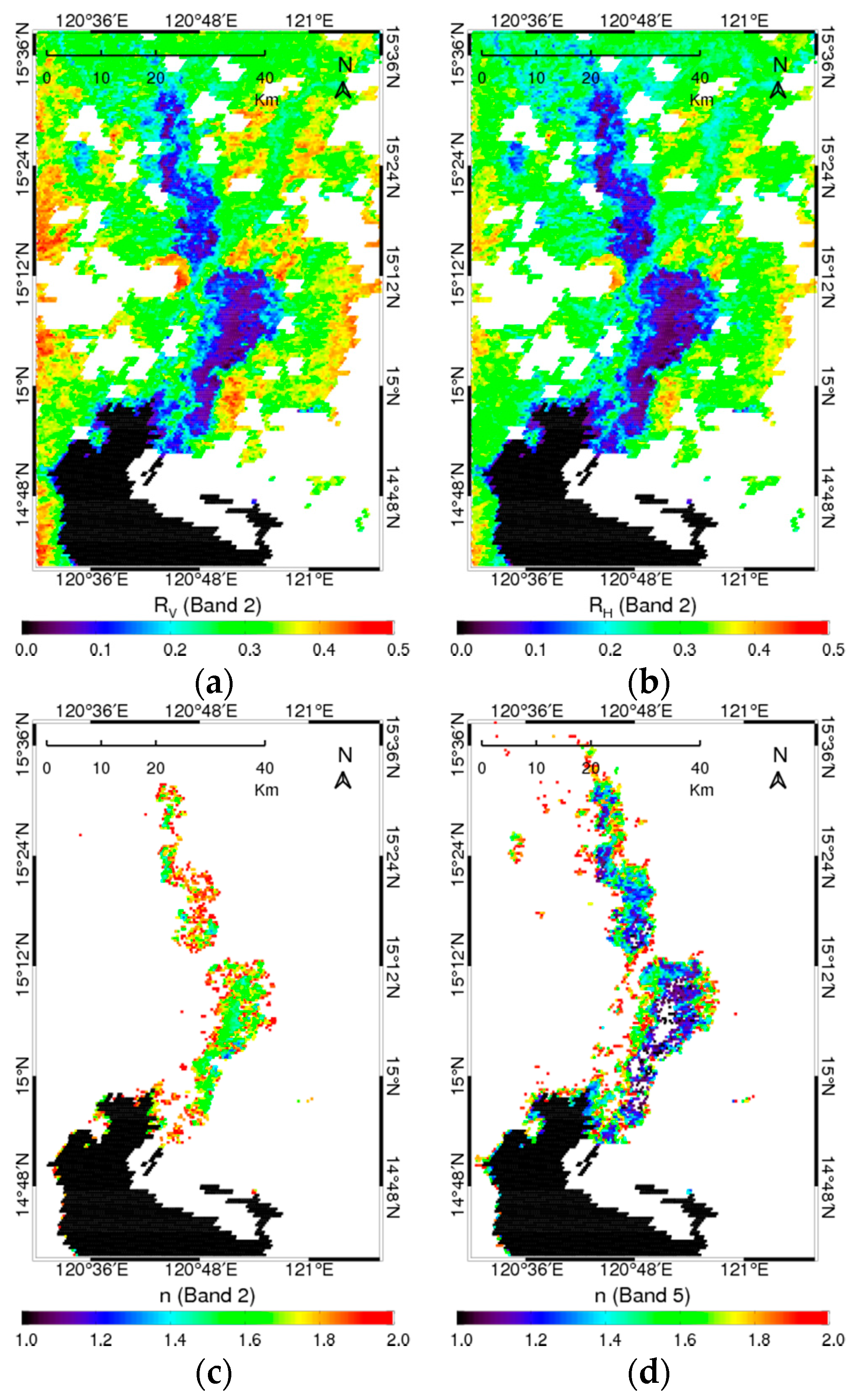
3.4. Refractive Index Retrieval Results

In this study, the error analysis of Equations (6) and (8) is performed for the flooding event. To support the result of an RGB combination, the refractive index is retrieved and validated for soil and water in these spectral bands.
Figure 10 shows the error of polarized reflectivities between the Fresnel equation, the Hong approximation, and the ASH approximation for soil and water in the VIS bands. In this case, the refractive index of the soil at 0.56 μm and water at 0.4 μm is found to be n ^ = 1 . 405 + 0 . 01 i [83] and n ^ = 1 . 339 + 1 . 86 × 10 9 i [81], respectively. Soil has a relatively larger value for the imaginary part of the refractive index than water in this wavelength. However, the analytical approximation exhibits a good agreement with the Fresnel equation from nadir to about 60° for soil and water. The Hong approximation shows agreement at around nadir and 45° viewing angles.
Figure 11 shows the error of the retrieved refractive indexes from the Fresnel equation, Hong approximation (Equation (6)), and ASH approximation (Equation (8)) for soil and water. In the case of the Fresnel equation, the error originates from the inversion method (Equation (10)), which greatly depends on the incidence angle, in good agreement with previous work [85]. In order to retrieve n (refractive index value for soil and water in VIS band), the analytical approximation is used and shows accurate results for simulating the Fresnel equation from nadir to about 55°, with an error of approximately 20%. The Hong approximation only appears to be accurate at around nadir and 45° viewing angles. The retrieval uncertainty in this case is primarily due to the inversion method (Equation (10)).
The real values of the refractive index for dry silica, calcite, soil, pure water, and seawater are 1.48 [86,87], 1.60 [86,88], 1.4 [83], and 1.33 [81], respectively. In this case, the incidence angles of MODIS data range from nadir to 30°. Figure 12 shows the result of part of the surface refractive index using the new combination of RGB 6-5-2bands. Figure 12a,b show the decomposed components of surface reflectivity for V- and H-polarizations, respectively. As mentioned previously, these bands were selected from a histogram analysis for RGB imagery flood detection, because they show high sensitivity to water absorption. Thus, the error of retrieved n due to the inversion methods is approximately 40% for the Hong approximation, and within 10% for the ASH approximation. As for the ASH approximation, the n value in the inundation area is retrieved from 1.6 to 2.0, as shown in Figure 12c. This value is relatively higher than that of the soil-water mixture. However, for the Hong approximation, the estimated n value in the inundation area ranges from 1.3 to 1.6, as shown in Figure 12d. In contrast, the values for vegetation and bare soil are greater than 1.6. This result is congruent because water is known to have a relatively lower value than that of soil. Accordingly, the refractive indexes of the flood area are generally less than 1.6 in the NIR wavelength, because of the high portion of water in the soil-water mixture. The larger error in the analytical approximation may be caused by several assumptions that were made, including the assumption of a specular surface, which ignores the effects of surface roughness, and the uncertainty of the refractive index inversion method. Figure 12e,f show the n values for bands 5 and 6, respectively. These results were useful for understanding the flood events using the new RGB composite imagery, as the color saturation of the RGB image was based on the surface reflectivities, which in turn depend on the refractive index values of the surfaces.

4. Conclusions

According to the recent increase in the frequency and magnitude of natural hazards such as flooding events, satellite remote sensing has become more valuable for disaster monitoring and relief efforts from the beginning to post-crisis of an event through space. For flood detection, much of the pioneering work on satellite remote sensing, including VIS and NIR sensors such as AVHRR and MODIS, has been done during the past three decades. Estimations of flooded areas serve as important input information for the models used for determining the extent of natural disasters and for making decisions regarding the recovery plans for the damaged areas. In particular, MODIS onboard the Aqua and Terra satellites is very useful for mapping the inundation area. In this study, the suitability of RGB composite image techniques for flood mapping based on the MODIS data is assessed for the flood area with a flood event at Pampanga River in the Philippines, in 2015. Methodologically, the RGB composite imagery of the MODIS 6-5-2 bands among many combinations of bands is suggested, because of their spectral sensitivity to distinguish water and soil/vegetation. The total flood area was estimated as being 499.5 km2 and is compared to the SAR analysis results of 483.3 km2, within a reasonable level of uncertainty. In addition, the RGB estimation is supported by the retrieval of the refractive index in the inundation area. The n value of the refractive index in the inundation area is estimated from 1.3 to 1.6 using the Hong approximation, and from 1.6 to 2.0 using the ASH approximation. The error in the estimated value may be caused by several assumptions that were made, including the assumption of a specular surface, which ignores the effects of surface roughness and the uncertainty of the refractive index inversion method.
Consequently, this study provides a useful RGB imagery technique for mapping flood events using a physical validation based on the refractive index. The technique can be applied to a variety of spectral ranges from ultraviolet to microwave wavelengths.

Acknowledgments

The authors thank anonymous reviewers for helpful and constructive comments on the manuscript. This study is supported by the ‘Development of Geostationary Meteorological Satellite Ground Segment Program’ funded by the National Meteorological Satellite Center (NMSC) of the Korea Meteorological Administration (KMA), and the grant (14AWMP-B082564-01) from ’Advanced Water Management Research Program’ funded by Ministry of Land, Infrastructure and Transport (MOLIT) of Korean government.

Author Contributions

Sungwook Hong conceived and designed the experiments; Hyun-Ju Ban performed the experiments and analyzed the data; Young-Joo Kwon, Hayan Shin, and Han-Sol Ryu contributed to data acquisition, the literature review, and discussions; Sungwook Hong and Hyun-Ju Ban wrote the paper.

Conflicts of Interest

The authors declare no conflict of interest.

References

  1. Giustarini, L.; Hostache, R.; Matgen, P.; Schumann, G.; Bates, P.D.; Mason, D.C. A change detection approach to flood mapping in urban areas using TerraSAR-X. IEEE Trans. Geosci. Remote Sens. 2013, 51, 2417–2430. [Google Scholar] [CrossRef]
  2. Martinis, S.; Twele, A.; Voigt, S. Towards operational near-real time flood detection using a split-based automatic thresholding procedure on high resolution TerraSAR-X data. Nat. Hazards Earth Syst. Sci. 2009, 9, 303–314. [Google Scholar] [CrossRef]
  3. Martinis, S.; Twele, A. A hierarchical spatio-temporal Markov model for improved flood mapping using multi-temporal X-band SAR data. Remote Sens. 2010, 2, 2240–2258. [Google Scholar] [CrossRef]
  4. Mason, D.C.; Davenport, I.J.; Neal, J.C.; Schumann, G.J.-P.; Bates, P.D. Near real-time flood detection in urban and rural areas using high-resolution Synthetic Aperture Radar images. IEEE Trans. Geosci. Remote Sens. 2012, 50, 3041–3052. [Google Scholar] [CrossRef]
  5. Schumann, G.; di Baldassarre, G.; Alsdorf, D.; Bates, P.D. Near real-time flood wave approximation on large rivers from space: Application to the River Po, Italy. Water Resour. Res. 2010, 46, 1–8. [Google Scholar] [CrossRef]
  6. Pulvirenti, L.; Pierdicca, N.; Chini, M.; Guerriero, L. An algorithm for operational flood mapping from Synthetic Aperture Radar (SAR) data using fuzzy logic. Nat. Hazards Earth Syst. Sci. 2011, 11, 529–540. [Google Scholar] [CrossRef]
  7. Brisco, B.; Touzi, R.; van der Sanden, J.J.; Charbonneau, F.; Pultz, T.J.; D’Iorio, M. Water resource applications with RADARSAT-2—A preview. Int. J. Digit. Earth 2008, 1, 130–147. [Google Scholar] [CrossRef]
  8. Brisco, B.; Short, N.; van der Sanden, J.; Landry, R.; Raymond, D. A semi-automated tool for surface water mapping with RADARSAT-1. Can. J. Remote Sens. 2009, 35, 336–344. [Google Scholar] [CrossRef]
  9. Smith, L.C. Satellite remote sensing of river inundation area, stage, and discharge: A review. Hydrol. Process. 1997, 11, 1427–1439. [Google Scholar] [CrossRef]
  10. Campbell, J.B. Introduction to Remote Sensing; The Guilford Press: New York, NY, USA, 2002; p. 206. [Google Scholar]
  11. White, L.; Brisco, B.; Dabboor, M.; Schmitt, A.; Pratt, A. Collection of SAR Methodologies for Monitoring Wetlands. Remote Sens. 2015, 7, 7615–7645. [Google Scholar] [CrossRef]
  12. Brakenridge, G.; Anderson, E.; Nghiem, S.; Caquard, S.; Shabaneh, T. Flood warnings, flood disaster assessments, and flood hazard reduction: The roles of orbital remote sensing. In Proceedings of the 30th International Symposium on Remote Sensing of the Environment, Honolulu, HI, USA, 10–14 November 2003; p. 4. [Google Scholar]
  13. France, M.J.; Hedges, P.D. A hydrological comparison of Landat TM, Landsat MSS, and black and white aerial photography. In Proceedings of the Seventh International Symposium on Remote Sensing for Resources Development and Environmental Management ISPRS Commission VII, Enschede, The Netherland, 25–29 August 1986. [Google Scholar]
  14. Jensen, J.R.; Hodgson, M.E.; Christensen, E., Jr.; Mackey, H.E.; Tinney, L.R.; Sharitz, R. Remote sensing inland wetlands: A multispectral approach. Photogramm. Eng. Remote Sens. 1986, 52, 87–100. [Google Scholar]
  15. Watson, J.P. A visual interpretation of a Landsat mosaic of the Okavango Delta and surrounding area. Remote Sens. Environ. 1991, 35, 1–9. [Google Scholar] [CrossRef]
  16. Blasco, F.; Bellan, M.F.; Chaudhury, M.U. Estimating the extent of floods in Bangladesh using SPOT data. Remote Sens. Environ. 1992, 39, 167–178. [Google Scholar] [CrossRef]
  17. Pope, K.O.; Rey-Benayas, J.M.; Paris, J.F. Radar remote sensing of forest and wetland ecosystems in the Central American tropics. Remote Sens. Environ. 1994, 48, 205–219. [Google Scholar] [CrossRef]
  18. Vila da Silva, J.S.; Kux, H.J.H. Thematic mapper and GIS data integration to evaluate the flooding dynamics within the Panatal. In Proceedings of the International Geoscience and Remote Sensing Symposium, Mato Grosso do Sul State, Brazil, 26–29 May 1992; pp. 1478–1480. [Google Scholar]
  19. Hallberg, G.R.; Hoyer, B.E.; Rango, A. Application of ERTS-1 imagery to flood inundation mapping. In Proceedings of the Symposium on Significant Results Obtained from the Earth Resources Satellite-1, New Carrollton, MD, USA, 5–9 March 1973; pp. 745–753. [Google Scholar]
  20. Rango, A.; Salomonson, V.V. Regional flood mapping from space. Water Resour. Res. 1974, 10, 473–484. [Google Scholar] [CrossRef]
  21. Morrison, R.B.; Cooley, M.E. Assessment of flood damage in Arizona by means of ERTS-1 imagery. In Proceedings of the Symposium on Significant Results Obtained from the Earth Resources Satellite-1, New Carrollton, MD, USA, 5–9 March 1973; pp. 755–760. [Google Scholar]
  22. McGinnis, D.F.; Rango, A. Earth resources satellite systems for flood monitoring. Geophys. Res. Lett. 1975, 2, 132–135. [Google Scholar] [CrossRef]
  23. Deutsch, M. Optical Processing of ERTS Data for Determining Extent of the 1973 Mississippi River Flood; U.S. Geol. Surv. Prof. Pap. 929, ERTS-1, a New Window on Our Planet; United States Government Printing Office: Washington, DC, USA, 1976; pp. 209–222.
  24. Morrison, R.B.; White, P.G. Monitoring Flood Inundation; U.S. Geol. Surv. Prof. Pap. 929, ERTS-1, A New Window on Our Planet; 1976; pp. 196–208. [Google Scholar]
  25. Ali, A.; Quadir, D.A.; Huh, O.K. Study of river flood hydrology in Bangladesh with AVHRR data. Int. J. Remote Sens. 1989, 10, 1873–1891. [Google Scholar] [CrossRef]
  26. Barton, I.J.; Bathols, J.M. Monitoring floods with AVHRR. Remote Sens. Environ. 1989, 30, 89–94. [Google Scholar] [CrossRef]
  27. Gale, S.J.; Bainbridge, S. The floods in eastern Australia. Nature 1990, 345, 767. [Google Scholar] [CrossRef]
  28. Rasid, H.; Pramanik, M.A.H. Areal extent of the 1988 flood in Bangladesh: How much did the satellite imagery show? Nat. Hazards 1993, 8, 189–200. [Google Scholar] [CrossRef]
  29. Sheng, Y.; Gong, P.; Xiao, Q. Quantitative dynamic flood monitoring with NOAA AVHRR. Int. J. Remote Sens. 2001, 22, 1709–1724. [Google Scholar] [CrossRef]
  30. Tucker, C.J. Red and photographic infrared linear combinations for monitoring vegetation. Remote Sens. Environ. 1979, 8, 127–150. [Google Scholar] [CrossRef]
  31. Domenikiotis, C.; Loukas, A.; Dalezios, N.R. The use of NOAA/AVHRR satellite data for monitoring and assessment of forest fires and floods. Nat. Hazards Earth Syst. Sci. 2003, 3, 1–14. [Google Scholar] [CrossRef]
  32. MCFeeters, S.K. The use of normalized difference water index (NDWI) in the delineation of open water features. Int. J. Remote Sens. 1996, 17, 1425–1432. [Google Scholar] [CrossRef]
  33. Gao, B.C. NDWI—A normalized difference water index for remote sensing of vegetation liquid water from space. Remote Sens. Environ. 1996, 58, 257–266. [Google Scholar] [CrossRef]
  34. Xiao, X.; Boles, S.; Frolking, S.; Salas, W.; Moore, B., III; Li, C. Observation of flooding and rice transplanting of paddy rice fields at the site to landscape scales in China using vegetation sensor data. Int. J. Remote Sens. 2002, 23, 3009–3022. [Google Scholar] [CrossRef]
  35. Ho, T.K.L.; Umitsu, M.; Yamaguchi, Y. Flood hazard mapping by satellite images and SRTM DEM in the Vu Gia—Thu Bon alluvial plain central Vietnam. Int. Arch. Photogramm. Remote Sens. Spat. Inf. Sci. 2010, 38, 275–280. [Google Scholar]
  36. Xu, H. Modification of normalised difference water index (NDWI) to enhance open water features in remotely sensed imagery. Int. J. Remote Sens. 2006, 27, 3025–3033. [Google Scholar] [CrossRef]
  37. Ning, L.; Liu, H.; Bao, A. Identification of inundation hazard zones in Manas Basin, China, using hydrodynamic modeling and remote sensing. J. Water Resour. Prot. 2013, 5, 469–473. [Google Scholar] [CrossRef]
  38. Kumar, R.; Acharya, P. Flood hazard and risk assessment of 2014 floods in Kashmir Valley: A space-based multisensor approach. Nat. Hazards 2016, 84, 437–464. [Google Scholar] [CrossRef]
  39. Li, R.R.; Kaufman, Y.J.; Hao, W.M.; Salmon, J.M.; Gao, B.C. A technique for detecting burn scars using MODIS data. IEEE Trans. Geosci. Remote Sens. 2004, 42, 1300–1308. [Google Scholar]
  40. Roy, D.; Lewis, P.E.; Justice, C.O. Burned area mapping using multi-temporal moderate spatial resolution data—A bi-directional reflectance model-based expectation approach. Remote Sens. Environ. 2002, 83, 263–286. [Google Scholar] [CrossRef]
  41. Chen, Y.; Huang, C.; Ticehurst, C.; Merrin, L.; Thew, P. An evaluation of MODIS daily and 8-day composite products for floodplain and wetland inundation mapping. Wetlands 2013, 33, 823–835. [Google Scholar] [CrossRef]
  42. Huang, C.; Chen, Y.; Wu, J. Mapping spatio-temporal flood inundation dynamics at large river basin scale using time-series flow data and MODIS imagery. Int. J. Appl. Earth Obs. Geoinf. 2014, 26, 350–362. [Google Scholar] [CrossRef]
  43. Lensky, I.M.; Rosenfeld, D. Clouds-aerosols-precipitation satellite analysis tool (CAPSAT). Atmos. Chem. Phys. 2008, 8, 6739–6753. [Google Scholar] [CrossRef]
  44. Dao, P.D.; Liou, Y.-A. Object-based flood mapping and affected rice field estimation with Landsat 8 OLI and MODIS data. Remote Sens. 2015, 7, 5077–5097. [Google Scholar] [CrossRef]
  45. Kwak, Y.; Arifuzzanman, B.; Iwami, Y. Prompt proxy mapping of flood damaged rice fields using MODIS-derived indices. Remote Sens. 2015, 7, 15969–15988. [Google Scholar] [CrossRef]
  46. Ticehurst, C.; Guerschman, J.P.; Chen, Y. The strengths and limitations in using the daily MODIS open water likelihood algorithm for identifying flood events. Remote Sens. 2014, 6, 11791–11809. [Google Scholar] [CrossRef]
  47. Spurr, R. A new approach to the retrieval of surface properties from earthshine measurements. J. Quant. Spectrosc. Radiat. Transf. 2004, 83, 14–46. [Google Scholar] [CrossRef]
  48. Warren, S.G. Optical constant of ice from the ultraviolet to the microwave. Appl. Opt. 1984, 23, 1206. [Google Scholar] [CrossRef]
  49. Aas, E. Refractive index of phytoplankton derived from its metabolite composition. J. Plankton Res. 1996, 18, 2223–2249. [Google Scholar] [CrossRef]
  50. Kaufman, Y.J.; Herring, D.D.; Ranson, K.J.; Collatz, G.J. Earth observing system AM1 mission to Earth. IEEE Trans. Geosci. Remote Sens. 1998, 36, 1045–1055. [Google Scholar] [CrossRef]
  51. Masuoka, E.; Fleig, A.; Wolfe, R.E.; Patt, F. Key characteristics of the MODIS data products. IEEE Trans. Geosci. Remote Sens. 1998, 36, 1313–1323. [Google Scholar] [CrossRef]
  52. Gupta, R.P.; Banerji, S. Monitoring of reservoir volume using Landsat data. J. Hydrol. 1985, 77, 159–170. [Google Scholar] [CrossRef]
  53. National Aeronautics and Space Administration (NASA) Jet Propulsion Laboratory (JPL). Available online: http://speclib.jpl.nasa.gov/documents/jhu_desc/ (accessed on 28 July 2016).
  54. Scientific Data Hub—Copernicus. Available online: https://www.scihub.copernicus.eu/dhus/#/home/ (accessed on 25 September 2016).
  55. Otsu, N. A threshold selection method from gray-level histogram. IEEE Trans. Geosci. Remote Sens. 1979, 9, 62–66. [Google Scholar] [CrossRef]
  56. Ford, A.; Roberts, A. Colour Space Conversions; Westminster University: London, UK, 1998. [Google Scholar]
  57. Bourke, P. RGB Colour Space—Lists of RGB Values for Named Colours; Swinburne University of Technology: Melbourne, Australia, 1995; Available online: http://paulbourke.net/texture_colour/colourspace/ (accessed on 11 May 2016).
  58. Umari, M.H.; Ghodgaonkar, D.K.; Varadan, V.V. A free-space bistatic calibration technique for the measurement of parallel and perpendicular reflection coefficients of planar samples. IEEE Trans. Geosci. Remote Sens. 1991, 40, 19–24. [Google Scholar] [CrossRef]
  59. Huang, Y.; Nakhkash, M. Characterization of layered dielectric medium using reflection coefficient. Electron. Lett. 1998, 34, 1207–1208. [Google Scholar] [CrossRef]
  60. Tousey, R. On calculating the optical constants from reflection coefficients. J. Opt. Soc. Am. 1939, 29, 235–238. [Google Scholar] [CrossRef]
  61. Hong, S. Retrieval of refractive index over specular surfaces for remote sensing applications. J. Appl. Remote Sens. 2009, 3, 033560. [Google Scholar] [CrossRef]
  62. Hong, S. Detection of Asian dust (Hwangsa) over the Yellow sea by decomposition of unpolarized infrared reflectivity. Atmos. Environ. 2009, 43, 5887–5893. [Google Scholar] [CrossRef]
  63. Hong, S.; Shin, I.; Ou, M. Comparison of the ISEM infrared sea-surface emissivity model with a physical emissivity model. J. Atmos. Ocean. Technol. 2010, 27, 345–352. [Google Scholar] [CrossRef]
  64. Hong, S. Surface roughness and polarization ratio in microwave remote sensing. Int. J. Remote Sens. 2010, 31, 2709–2716. [Google Scholar] [CrossRef]
  65. Hong, S. Global retrieval of small-scale roughness over land surfaces at microwave frequency. J. Hydrol. 2010, 389, 121–126. [Google Scholar] [CrossRef]
  66. Hong, S.; Shin, I. A physically-based inversion algorithm for retrieving soil moisture in passive microwave remote sensing. J. Hydrol. 2011, 405, 24–30. [Google Scholar] [CrossRef]
  67. Hong, S. Detection of small-scale roughness and refractive index of sea ice in passive satellite microwave remote sensing. Remote Sens. Environ. 2010, 114, 1136–1140. [Google Scholar] [CrossRef]
  68. Hong, S.; Shin, I. Global trends of sea ice: small-scale roughness and refractive index. J. Clim. 2010, 23, 4669–4676. [Google Scholar] [CrossRef]
  69. Hong, S.; Shin, I. Wind speed retrieval based on sea surface roughness measurements from spaceborne microwave radiometers. J. Appl. Meteorol. Climatol. 2013, 52, 507–516. [Google Scholar] [CrossRef]
  70. Hong, S.; Seo, H.; Kwon, Y. A unique satellite-based sea surface wind speed algorithm and its application in tropical cyclone intensity analysis. J. Atmos. Ocean. Technol. 2016, 33, 1363–1375. [Google Scholar] [CrossRef]
  71. Hong, S.; Seo, H.; Kim, N.; Shin, I. Physical retrieval of tropical ocean surface wind speed under rain-free conditions using spaceborne microwave radiometers. Remote Sens. Lett. 2015, 6, 380–389. [Google Scholar] [CrossRef]
  72. Azzam, R.M.A. Direct relation between Fresnel’s interface reflection coefficients for the parallel and perpendicular polarizations. J. Opt. Soc. Am. 1979, 69, 1007–1016. [Google Scholar] [CrossRef]
  73. Azzam, R.M.A. Relations between amplitude reflectances and phase shifts of the p and s polarizations when electromagnetic radiation strikes interfaces between transparent media. Appl. Opt. 1979, 18, 1884–1886. [Google Scholar] [CrossRef] [PubMed]
  74. Azzam, R.M.A. Relationship between the p and s Fresnel reflection coefficients of an interface independent of angle of incidence. J. Opt. Soc. Am. 1986, 3, 928–929. [Google Scholar] [CrossRef]
  75. Hong, S. Polarization conversion for specular components of surface reflection. IEEE Trans. Geosci. Remote Sens. Lett. 2013, 10, 1469–1472. [Google Scholar] [CrossRef]
  76. Hong, S. Decomposition of unpolarized emissivity. Int. J. Remote Sens. 2010, 31, 2109–2114. [Google Scholar] [CrossRef]
  77. Wu, X.; Smith, W.L. Emissivity of rough sea surface for 8–13 μm: Modeling and verification. Appl. Opt. 1997, 36, 2609–2619. [Google Scholar] [CrossRef] [PubMed]
  78. Querry, M.R. On direct solution of the generalized Fresnel reflectance equations. J. Opt. Soc. Am. 1969, 59, 876–877. [Google Scholar] [CrossRef]
  79. Kildemo, M.; Bulkin, P.; Deniau, S.; Drévillon, B. Real time control of plasma deposited multilayers by multiwavelength ellipsometry. Appl. Phys. Lett. 1996, 68, 3395–3397. [Google Scholar] [CrossRef]
  80. Heitz, T.; Hofrichter, A.; Bulkin, P.; Drévillon, B. Real time control of plasma deposited optical filters by multiwavelength ellipsometry. J. Vac. Sci. Technol. 2000, 18, 1303–1307. [Google Scholar] [CrossRef]
  81. Hale, G.M.; Querry, M.R. Optical constants of water in the 200-nm to 200-μm wavelength region. Appl. Opt. 1973, 12, 555–563. [Google Scholar] [CrossRef] [PubMed]
  82. Zoloratev, V.M.; Demin, A.V. Optical constants of water over a broad range of wavelengths, 0.1 Ǻ—l m. Opt. Spectrosc. 1977, 43, 157. [Google Scholar]
  83. Liang, S. An investigation of remotely-sensed soil depth in the optical region. Int. J. Remote Sens. 1997, 18, 3395–3408. [Google Scholar] [CrossRef]
  84. Strahler, A.; Muchoney, D.; Borak, J.; Friedl, M.; Gopal, S.; Lambinet, E. MODIS BRDF/Albedo Product Algorithm Theoretical Basis Document; MOD43, Version 5.0; Boston University: Boston, MA, USA, 1999. [Google Scholar]
  85. Armaly, B.F.; Ochoa, J.G.; Look, D.C. Restrictions on the inversion of the Fresnel reflectance equations. Appl. Opt. 1972, 11, 2907–2910. [Google Scholar] [CrossRef] [PubMed]
  86. McCrone, W.C.; Draftz, R.G.; Delly, J.G. The Particles Atlas; Ann, A., Ed.; Ann Arbor Science Publishers: Ann Arbor, MI, USA, 1967. [Google Scholar]
  87. Hodgson, R.T.; Newkirk, D.D. Pyridine immersion: A technique for measuring the refractive index of marine particles. Proceedings of International Society for Optical Engineering, San Diego, CA, USA, 19 August 1975; pp. 62–64. [Google Scholar]
  88. Weast, R.C. Handbook of Chemistry and Physics; CRC: Cleveland, OH, USA, 1981. [Google Scholar]
Figure 1. (a) Location of the Pampanga River in the Philippines; (b) Locations of the Poyang and Dongting Lakes in China.
Remotesensing 09 00313 g001
Figure 2. MODIS true color images combining bands 1, 4, and 3. Panels (a,b) show the Pampanga River area, highlighting the surface conditions before (16 September 2015 at 02:20 UTC) and after (25 October 2015 at 02:25 UTC) the flooding event, respectively. Panels (c,d) show the Poyang and Dongting Lakes focusing on the surface conditions before (27 March 2016 at 03:00 UTC) and after (28 July 2016 at 02:40 UTC) the flood event, respectively.
Remotesensing 09 00313 g002
Figure 3. Reflectance values of clay, sand, loam, grass, snow, and water. These values range from 0.4 μm to 2.6 μm. MODIS spectral response functions corresponding to these values are also shown. The spectral data are obtained from NASA Jet Propulsion Laboratory [53].
Remotesensing 09 00313 g003
Figure 4. Backscattering coefficients of VV-polarizations observed from SENTINEL-1A (a) around the Pampanga River in the Philippines on 26 October 2015 at 21:46 UTC and (b) around the Poyang and Dongting Lakes in China on 3 August 2016 at 10:27 UTC.
Remotesensing 09 00313 g004
Figure 5. An outline of the research procedure.
Remotesensing 09 00313 g005
Figure 6. Surface reflectance histograms for MODIS bands (a) 1 to (g) 7 on 25 October 2015 around the Pampanga River basin, Philippines. Clear bimodal distributions appear in the histograms for bands 2, 5, and 6.
Remotesensing 09 00313 g006
Figure 7. RGB 6-5-2 images showing the Pampanga River in the Philippines (a) before the flooding on 16 September 2015 at 02:20 UTC and (b) after the flooding on 25 October 2015 at 02:25 UTC. The satellite data used is the same as that used in Figure 2. RGB 6-5-2 images of the Poyang and Dongting Lakes in China (c) before flooding on 27 March 2016 at 03:00 UTC and (d) after flooding on 28 July 2016 at 02:40 UTC.
Remotesensing 09 00313 g007aRemotesensing 09 00313 g007b
Figure 8. Backscattering coefficient images of VV-polarized SENTINEL-1A data (a) on 25 October 2015 around the Pampanga River basin, Philippines and (b) on 3 August 2016 at 10:27 UTC around the Poyang and Donting Lakes in China. Backscattering coefficient histograms (c) for case (a) and (d) for case (b). Otsu’s method was applied to determine the threshold values in both cases.
Remotesensing 09 00313 g008
Figure 9. Flood area estimations around the Pampanga River using (a) RGB 6-5-2 imagery and (b) SENTINEL-1A data. Flood area estimations around the Poyang and Dongting Lakes using (c) RGB 6-5-2 imagery and (d) SENTINEL-1A data.
Remotesensing 09 00313 g009
Figure 10. Errors in vertically polarized reflectivity ( R V ) and horizontally polarized reflectivity ( R H ) values between the Fresnel equation and the Hong approximation, and analytical approximation for (a) soil at 0.56 μm and (b) water at 0.4 μm.
Remotesensing 09 00313 g010
Figure 11. Error (%) in the retrieved refractive index (n) for (a) soil at 0.56 μm and (b) water at 0.4 μm.
Remotesensing 09 00313 g011
Figure 12. Retrieved V-and H-polarized reflectivities and refractive index over the flood area in the Pampanga River at band 2 using the Hong and ASH approximations. (a) R V , (b) R H , (c) n(ASH), (d) n(Hong), (e) n(Hong) at band 5, and (f) n(Hong) at band 6. Hong and ASH indicate Hong approximation and ASH approximation, respectively.
Remotesensing 09 00313 g012aRemotesensing 09 00313 g012b

