The Predictive Power of Different Projector-Augmented Wave Potentials for Nuclear Quadrupole Resonance

1
Department of Computational and Data Sciences, George Mason University, Fairfax, VA 22030, USA
2
Department of Physics and Astronomy, George Mason University, Fairfax, VA 22030, USA
3
Quantum Materials Center, George Mason University, Fairfax, VA 22030, USA
*
Author to whom correspondence should be addressed.
†
Current address: Data Analytics Department, MITRE Corporation, 7515 Colshire Drive, McLean, VA 22102, USA.
Crystals 2019, 9(10), 507; https://doi.org/10.3390/cryst9100507
Submission received: 8 August 2019
/
Revised: 12 September 2019
/
Accepted: 25 September 2019
/
Published: 28 September 2019
(This article belongs to the Special Issue NQR of Polymorphic Crystals)
Abstract
:The projector-augmented wave (PAW) method is used to calculate electric field gradients (EFG) for various PAW potentials. A variety of crystals containing reactive nonmetal, simple metal, and transition elements, are evaluated in order to determine the predictive ability of the PAW method for the determination of nuclear quadrupole resonance frequencies in previously unstudied materials and their polymorphs. All results were compared to experimental results and, where possible, to previous density functional theory (DFT) calculations. The EFG at the 14N site of NaNO2 is calculated by DFT for the first time. The reactive nonmetal elements were not very sensitive to the variation in PAW potentials, and calculations were quite close to experimental values. For the other elements, the various PAW potentials led to a clear spread in EFG values, with no one universal potential emerging. Within the spread, there was agreement with other ab initio models.
1. Background
Nuclear quadrupole resonance (NQR) spectroscopy is highly specific to the material as the frequencies directly depend on the intrinsic electric field gradient (EFG) at the nuclear site [1]. One strong hallmark of this specificity is the ability of NQR to distinguish between polymorphs of a crystal [2,3,4]. While potential applications of NQR are numerous, including pharmaceutical applications [5,6], detection of illicit substances [7,8,9], and fundamental materials exploration [10,11,12,13,14], among others, the ability to find the NQR frequencies of previously unstudied materials can be prohibitively time-consuming precisely because of the specificity of the technique.
Density functional theory (DFT) can be used to calculate the electric field gradient at the nucleus [15,16,17,18,19,20] and therefore the NQR frequencies, including those for different polymorphs [3,21]. In principle this can greatly reduce the search time for new NQR transitions, but in practice is limited by the quality of predictions that can be produced with DFT. To date, most DFT calculations of the EFG in different bulk-like materials have either been full-potential linearized augmented plane wave (FP-LAPW) calculations or employed the projector-augmented wave (PAW) method [21]. While both methods use a plane wave expansion for the electronic wave function, they differ in how they treat the electric potential generated by the nuclei. The full potential method does not alter the potential in any way while the PAW method instead uses a pseudopotential for the potential around the nuclei. A transformation is then used to convert the “pseudized” wave functions into all-electron wave functions that should, in principle, reproduce the FP-LAPW functions. The FP-LAPW method is more accurate but at the cost of being more computationally demanding, which limits the number of atoms that can be routinely handled. The accuracy of the PAW method, on the other hand, depends on the initial choice of pseudopotential.
The dependence of EFG predictions on the choice of PAW potential is demonstrated in this work. A commercially available DFT software which implements the PAW method, Vienna Ab-initio Simulation Package vasp [22,23,24,25], and their suite of PAW potentials were used for the calculations. The goal of the research was to establish how sensitive the computed EFG is to the choice of PAW potential for different bulk-like materials. The desired application is for the standardized prediction of NQR frequencies in previously unstudied materials, including polymorphic configurations, to ease in the search of NQR transition frequencies.
The choice of materials studied was largely motivated by the ability to compare these EFG predictions to experimental results as well as previous DFT calculations. In particular three of the materials, LiN, TiO, and CuO were chosen from the seminal work by Petrilli, et al. [16]; the last solid was further studied by more advanced full-potential models [26,27,28,29]. Within the group studied are two semiconducting oxides containing transition metal elements, TiO and CuO, and those containing only main group elements, LiN, which is an ionic conductor, and NaNO which is an ionic insulator. The last crystal was not studied by Petrilli et al. [16]. There are several reasons for including this last material: (1) the popularity of sodium nitrite as a standard on which to test pulse sequences in NQR, (2) the EFG at the nitrogen site has not been calculated through DFT methods, and (3) the EFG at the sodium site has been calculated [30] using DFT and the Hartree–Fock approximation in tandem with a linear combination of atomic orbitals basis set.
2. Methods
2.1. Computational Methods
We calculated the electronic structure and EFG of Cu2O, Li3N, TiO2 (rutile), and NaNO2 using first-principles DFT and employed the PBE form of the generalized gradient approximation (GGA) [31] for our exchange-correlation functional. Initial tests using the local density approximation (LDA) [32] for NaNO2 were also performed and compared to the PBE results in order to determine any dominant effects related to functional choice. Our calculations are based on the projector-augmented wave (PAW) potentials [33,34] implemented in vasp. For each compound we swept through all combinations of potentials and computed the EFG for each potential configuration, which we converged with respect to the number of k-points and the plane-wave energy cutoff. A high energy cutoff of 1000 eV was required for the plane waves for all compounds while coarser meshes were sufficient for the k-points. Specifically, we used for NaNO2, for Li3N, for TiO2, and for Cu2O.
Three different generations of PAW potentials are distributed with vasp and all our calculations employed version 5.4 of the PBE potentials. Within this subset of PAW potentials several choices are available for each atomic species that are grouped by the following traits: (1) hard or soft potentials—these labels refer to whether the initial pseudopotentials used as part of the PAW method have either a small (hard) or large (soft) radius cutoff when defining the potential around the atomic sites. A smaller cutoff is generally more accurate but requires the use of a much higher plane-wave energy cutoff in order to converge the total energy and EFG. (2) sv and pv potentials—these are potentials that include s or p semicore states as part of the basis set for the valence bands. (3) GW potentials—these potentials are designed to better reproduce scattering properties at higher energies and are recommended for use in GW calculations. G refers to Green’s function and W refers to the screen Coulomb interaction [35]. These potentials are also expected to perform well when used for standard electronic structure calculations. Any results that we label with GW refer to calculations that used these potentials, not to calculations based on the GW approximation. (4) AE potentials—this refers to an accurate, alternative version of a potential which stands for “all electron” [36]. (5) standard potentials—this refers to a potential that does not include any of these aforementioned features.
Following the seminal work by Petrilli et al. [16], the crystal structures were not optimized. Instead the crystal structures for all reported compounds were all sourced from X-ray diffraction experiments. The structural information used in the vasp calculations are summarized in Table 1.
We use the following distance-type metric to compare our calculated EFG tensors with experimental results,
where , , and refer to our calculated results and , , and refer to an experimentally derived EFG obtained from the literature. The tensor components are taken from the diagonalized EFG tensor that satisfies , unless otherwise noted.
2.2. Relationship between EFG and NQR Frequencies
The relationship between NQR frequencies and the electric field gradient depend on the spin I of the nucleus. The nuclei addressed in the article range from spin-1 to spin-5/2. The frequencies are obtained from differences in energy eigenvalues of the Electric Quadrupolar Hamiltonian [38],
where Q is the quadrupole moment, e is the elementary charge, and the principle axes frame is assumed with . For spin-1 and spin-3/2 nuclei, analytic solutions exist for the NQR frequencies, but for spin-5/2 there are only numerical solutions for , where the asymmetry parameter is defined as .
2.2.1. Spin-1
For spin-1, for example N, there are three frequencies [39]:
where . These are easy to invert to get the electric field gradient from the NQR frequencies, but it must be kept in mind that the experimental frequency does not retain a sign and therefore cannot be used to determine the sign of the gradient. In this case it has been adopted to follow the sign predicted by DFT. Often the frequencies are rewritten in terms of two constants, the quadrupole coupling constant , and the asymmetry parameter introduced earlier as , such that . Using these definitions in Equation (3), one obtains
The linear connection between the field gradient and the frequency is somewhat obscured, however, by this notation.
For NaNO2, 14N-NQR frequencies at 300 K were obtained by Sauer et al. [39], and were used to calculate the electric field gradient. For Li3N, 14N-NMR frequencies at 290 K [40] were used to calculate the gradients; because of the hexagonal symmetry of Li3N it was expected, and subsequently confirmed by experiment, that at the nitrogen site. In both cases, [41], and the error in the gradient calculated by experiment is less than 1%.
2.2.2. Spin-3/2
For spin 3/2, for example Li, Na, and Cu, there is only one NQR transition frequency,
since the quantum states split into a pair of doubly degenerate energy levels [1]. It is clear that the frequency does not depend on the sign of the gradient, and also that it is not possible to find all three values of the gradient. For some structures, the symmetry of the crystal implies that and therefore . With this assumption, can be calculated, as was done for Cu in Cu2O at 295 K [42]. The DFT calculations support the symmetry argument for 63Cu in Cu2O.
Using NMR, instead of NQR, it is possible to get all three gradients to compare to DFT calculations. This was done for 7Li in LiN3 at 290 K by Differt et al. [40], and for 23Na in NaNO2 at 293 K by Weiss [43]. All quadrupole moments, in fm, were taken from Pyykkö [41,44], , , , and used to calculate the electric field gradients.
2.2.3. Spin-5/2
For spin-5/2, for example 47Ti and 17O, only a numerical solution for the NQR frequencies can be found. The two dominant NQR frequencies are calculated numerically and reported in the results section. There is a third transition which is weaker and occurs at the sum of the two dominant frequencies. The quadrupole moments are from Pyykkö [41]: fm, fm.
Experimental data for TiO2 was taken from Gabathuler et al. [45]. This reference does not explicitly give the temperature of the experiment, but presumably would be room temperature by its omission.
3. Results and Discussion
The full gradient is visualized by plotting the and components as a function of the component, with . In the following graphs, the different PAW potentials for the nuclear site where the EFG is calculated are distinguished by different colors as is reflected in the legend. For most materials, off-site potentials were also varied. Since this was a secondary effect, and for readability, different symbols were not assigned for these off-site potentials. Therefore multiple points exist for each on-site potential calculated. Where relevant, the secondary effect of these off-site potential choices are discussed in the text.
Also plotted in the graphs are experimental values, along with literature values of the EFG. Of particular importance is comparison with methods that are more holistic than the PAW method, namely LAPW or Hartree–Fock methods. Where multiple literature values exist, the most recent and the most closely related to our method were adopted for comparison. EFG calculations by the PAW method were first done by Petrilli et al. [16]. In this work, which predates vasp, different versions of the functionals LDA and GGA parametrization were employed. The PAW potentials of vasp are created following the recipe laid out by Kresse et al. [34]. To distinguish between literature PAW values from Petrilli et al. and our reported PAW values, we have marked literature PAW values as “Pet. PAW” in the legends.
Lastly, NQR frequencies due to the different potentials are calculated from the computed gradients and literature quadrupole moments, according to Section 2.2. They are visualized directly below each gradient plot. The plots are one-dimensional horizontally, however the markers have been randomly spread vertically in order to reveal any overlapping data points. The colors and marker shapes are consistent with the corresponding gradient plot.
This discussion is divided into the following classes: reactive nonmetals, nitrogen and oxygen; simple metals, lithium and sodium; and transition metal elements, titanium and copper.
3.1. Reactive Nonmetals
The reactive nonmetals studied had the following PAW potentials available: standard, hard, soft, and GW including both hard and soft varieties. Nitrogen data is shown in Figure 1 for NaNO2 and in Figure 2 for Li3N, while oxygen data for TiO2 is in Figure 3. For all sites studied the PAW potentials form a continuum of values, which are relatively close to the experimentally derived value, as characterized by . This relatively close agreement between experiment and DFT calculations is extended to NQR frequencies; the largest deviation from experiment for the highest NQR frequency of each site is close to the largest value for that site.
There were subtle differences between the different materials. The calculated values overestimate the EFG for the nitrogen sites, but are nearly centered on the EFG for oxygen in TiO2. For oxygen in TiO2 and nitrogen in Li3N, there is a small, but noticeable, spread in EFG values due to the choice of PAW potential for the other site, that is titanium and lithium. For readability, labels for the other site were not included in the graphs. There is, however, a common trend. For TiO2 and for a fixed PAW potential on the oxygen, the sv and pv PAW potentials on the titanium site consistently gave smaller at the oxygen site than the standard potential. In a similar manner, for Li3N, those lithium PAW potentials with sv or AE GW consistently gave smaller at the nitrogen site than the other potentials.
For Li3N and TiO2, electric field gradients were also calculated with the full-potential (LAPW). The values calculated with the PAW method agree well with those values. The nitrogen site for NaNO2 had no previous computational work done. For this site, we explored the effects of using a different functional. The results from the LDA functional were quite similar to the PBE functional, as shown in Figure 1.
3.2. Simple Metals
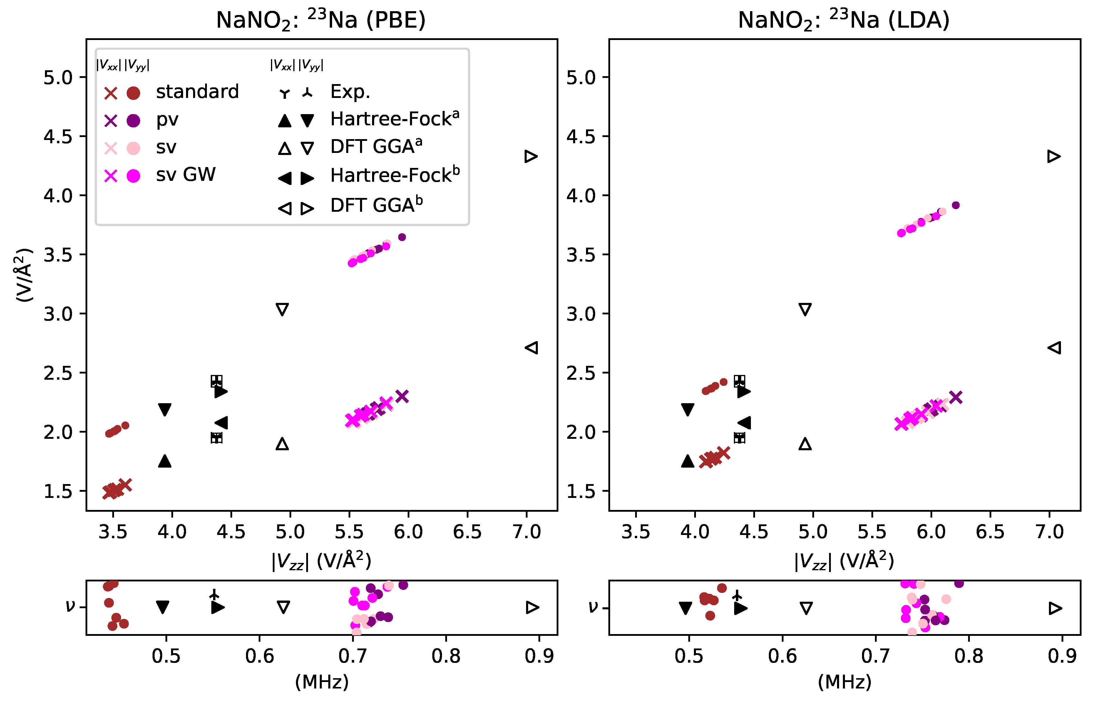
For simple metals, the treatment of semicore electrons as valence, which includes sv, sv GW, pv, and AE GW potentials, gives significantly different results than those PAW potentials that treat semicore electrons in the standard way. The latter includes the standard and GW potentials. Data for the sodium site in NaNO2 is shown in Figure 4, while data for the lithium sites in Li3N is shown in Figure 5. In both cases, the calculated results encompass the experimental value. For the sodium site, however, the standard potential underestimates the gradient by , while for the lithium sites the standard and GW potentials severely overestimate the gradient . In contrast, the treatment of semicore electrons as valence overestimates the gradient by for the sodium site, while for the lithium sites the sv potential underestimates the gradient by about the same amount. The sv GW and AE GW potentials, however, give EFG values that are very close to the experimental value for the lithium sites, . The same basic patterns, and the size of the deviation from experiment, are found in the calculated NQR frequencies.
For the sodium site, the literature values have a spread comparable to our PAW calculations. The methods presented in Ref. [30] rely heavily on the choice of the orbital basis set, which is why there is a spread in literature values. However, unsurprisingly, the Hartree–Fock calculations are the closest to experiment compared to any of the presented DFT methods. Similarly, the LAPW calculation is quite close to experiment for the lithium sites.
In addition, we also explored the effects of using a different functional for the sodium site. As seen in Figure 4, the results from the LDA functional showed the same basic distribution pattern with PAW potential as the PBE functional. The treatment of semicore electrons as valence gives about the same overestimation of the EFG for both functionals. The standard potential also underestimates the EFG in both cases, but not as severely in the case of the PBE functional.
3.3. Transition Metal Elements
The 3d transition elements within the two semi-conducting oxides show very different behavior. As shown in Figure 3, titanium PAW potentials divide neatly into two camps: one that treats s or p electrons as valence and the standard PAW potential. The former agrees well with other theoretical predictions as well as with experimental results; the latter is too high by . Ref. [47] suggests for titanium the use of the pv PAW potential for general purposes, as opposed to the standard potential, which is born out quite nicely here for EFG calculation.
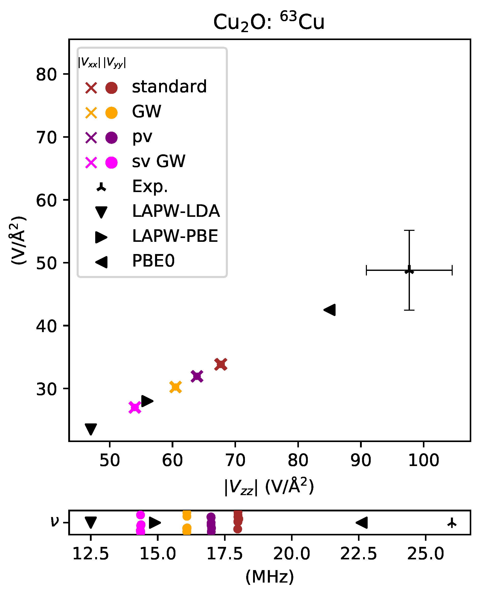
As shown in Figure 6, for copper in Cu2O, all the PAW potentials significantly underestimate the EFG value. They are, however, in good company with full potential predictions made with LAPW using the popular LDA and PBE functionals. Cu2O has become a stringent test of new DFT methods due in part to this inconsistency [29]. Only the use of a hybrid functional, which incorporates a fraction of exact exchange, brings the calculation close to the experimental result, as shown in Figure 6 for the PBE0 functional [27]. This particular hybrid functional is also offered in vasp, but was not explored as part of this work. Hybrid functionals in general come at the cost of computational complexity [48], and the focus of this work was on predictions done while maintaining computational efficiency.
For both copper in Cu2O and titanium in TiO2, the distribution of NQR frequencies closely mirror the electric field gradient results.
4. Conclusions
The EFGs computed using various PAW potentials, as well as their corresponding NQR frequencies, were consistent with the results from more holistic approaches, like FP-LAPW or Hartree–Fock methods. In certain cases, for instance lithium in Li3N and titanium in TiO2, the spread in values for various PAW potentials compared to the more holistic approaches would give us some pause for preferring the PAW method unless a “good” PAW potential was known a priori. In the case of the lithium site, we note that the AE GW potential yielded results that were close both to the experimental and full potential results; this particular potential did not exist for any other of the atoms studied.
A similar spread in values with PAW potential was seen with LDA functional as with the PBE functional. The comparison between functionals was, however, not the focus of this study and was only done with the nitrogen and sodium sites in NaNO2. In all other materials only the PBE functional was used. From this limited sample, we conclude that as far as the non-empirical LDA and PBE functionals are concerned, the choice of PAW potential is the dominant factor in determining the predicted value for the NQR frequency.
In general, the calculated EFGs were relatively insensitive to the choice of PAW potential for atoms surrounding the site of interest. For some sites, oxygen in TiO2 and nitrogen in NaNO2 and in Li3N, the EFG values were also insensitive to the choice of PAW potential at that site. In these cases, the discrepancy from experiment was small, . Notably the examples are reactive nonmetal elements from the 2nd row of the periodic table.
In contrast, for other sites there is a clear clustering of EFG based on the choice of PAW potential. The treatment of p or s semicore states as valence electrons is often the critically dividing factor. For example, when p or s semicore states are included in the valence, the EFG is
- overestimated by % for sodium in NaNO2,
- well-predicted, , for titanium in TiO2,
- underestimated by for lithium in Li3N with no other modifications of the potential,
and when they are not included in the valence, the EFG is
- underestimated by for sodium in NaNO2,
- overestimated by for titanium in TiO2,
- overestimated by for lithium in Li3N.
From the overall results it is clear that there is no universal potential that leads to satisfying EFG results, and therefore NQR frequencies, for all solids. For instance, the sv GW potential led to the best agreement with experimental results at the lithium sites in Li3N; the same potential also gives excellent agreement with experiment for the titanium site in TiO2. The use of the same potential, however, led to the worst agreement with experimental results in Cu2O. Another example was the standard potential, which gave EFG values closest (or nearly so) to experimental results for both sodium and nitrogen in NaNO2, nitrogen in Li3N, copper in Cu2O, but the worst (or nearly so) disagreement for lithium sites in Li3N and titanium in TiO2. In lieu of a universal potential, however, there are PAW potentials suggested in Ref. [47], namely the treatment of semicore p or s electrons as valence for lithium, sodium, and titanium and the standard potential for nitrogen, oxygen, and copper. Armed with these suggestions for compromise we found the EFG calculation came within ∼35% of the experimental value, and in most cases much closer. The corresponding NQR frequencies also came within ∼35% of the experimental value.
Author Contributions
Conceptualization, K.L.S.; data curation, J.N.A.; formal analysis, J.N.A., K.L.S. and J.K.G.; funding acquisition, K.L.S.; writing—original draft, J.N.A., K.L.S. and J.K.G.; writing—review, J.N.A., K.L.S. and J.K.G.; visualization, J.N.A.; supervision, K.L.S. and J.K.G.
Funding
This research was supported by the National Science Foundation under sponsor award number ECCS-1711118. J. N. Ansari acknowledges funding from the Quantum Materials Center at George Mason University.
Acknowledgments
All reported results in this study were run on ARGO, a research computing cluster provided by the Office of Research Computing at George Mason University, VA. (http://orc.gmu.edu). We would also like to gratefully acknowledge Yuri Mishin and Yi-Shen Lin for very helpful discussions regarding vasp.
Conflicts of Interest
The authors declare no conflict of interest.
References
- Suits, B.H. Nuclear quadrupole resonance spectroscopy. In Handbook of Applied Solid State Spectroscopy; Vij, D.R., Ed.; Springer: Boston, MA, USA, 2006; pp. 65–96. [Google Scholar] [CrossRef]
- Poleshchuk, O.; Latosińska, J.; Latosińska, M. Nuclear Quadrupole Resonance, Applications. In Encyclopedia of Spectroscopy and Spectrometry; Academic Press: Cambridge, MA, USA, 2016. [Google Scholar] [CrossRef]
- Seliger, J.; Žagar, V.; Apih, T.; Gregorovič, A.; Latosińska, M.; Olejniczak, G.A.; Latosińska, J.N. Polymorphism and disorder in natural active ingredients. Low and high-temperature phases of anhydrous caffeine: Spectroscopic (1H–14N NMR–NQR/14N NQR) and solid-state computational modelling (DFT/QTAIM/RDS) study. Eur. J. Pharm. Sci. 2016, 85, 18–30. [Google Scholar] [CrossRef]
- Trontelj, Z.; Lužnik, J.; Pirnat, J.; Jazbinšek, V.; Lavrič, Z.; Srčič, S. Polymorphism in Sulfanilamide: 14N Nuclear Quadrupole Resonance Study. J. Pharm. Sci. 2019, 108, 2865–2870. [Google Scholar] [CrossRef] [PubMed]
- Latosińska, J. Nuclear Quadrupole Resonance spectroscopy in studies of biologically active molecular systems—A review. J. Pharm. Biomed. Anal. 2005, 38, 577–587. [Google Scholar] [CrossRef]
- Barras, J.; Althoefer, K.; Rowe, M.D.; Poplett, I.J.; Smith, J.A.S. The Emerging Field of Medicines Authentication by Nuclear Quadrupole Resonance Spectroscopy. Appl. Magn. Reson. 2012, 43, 511–529. [Google Scholar] [CrossRef]
- Grechishkin, V.S.; Sinyavskii, N.Y. New technologies: Nuclear quadrupole resonance as an explosive and narcotic detection technique. Physics-Uspekhi 1997, 40, 393–406. [Google Scholar] [CrossRef]
- Yesinowski, J.P.; Buess, M.L.; Garroway, A.N.; Ziegeweid, M.; Pines, A. Detection of 14N and 35Cl in Cocaine Base and Hydrochloride Using NQR, NMR, and SQUID Techniques. Anal. Chem. 1995, 67, 2256–2263. [Google Scholar] [CrossRef]
- Garroway, A.N.; Buess, M.L.; Miller, J.B.; Suits, B.H.; Hibbs, A.D.; Barrall, G.A.; Matthews, R.; Burnett, L.J. Remote sensing by nuclear quadrupole resonance. IEEE Trans. Geosci. Remote. Sens. 2001, 39, 1108–1118. [Google Scholar] [CrossRef] [Green Version]
- Klanjsek, M.; Zorko, A.; Zitko, R.; Mravlje, J.; Jaglicic, Z.; Biswas, P.K.; Prelovsek, P.; Mihailovic, D.; Arcon, D. A high-temperature quantum spin liquid with polaron spins. Nat. Phys. 2017, 13, 1130 EP. [Google Scholar] [CrossRef]
- Yasuoka, H.; Kubo, T.; Kishimoto, Y.; Kasinathan, D.; Schmidt, M.; Yan, B.; Zhang, Y.; Tou, H.; Felser, C.; Mackenzie, A.P.; et al. Emergent Weyl Fermion Excitations in TaP Explored by 181Ta Quadrupole Resonance. Phys. Rev. Lett. 2017, 118, 236403. [Google Scholar] [CrossRef]
- Ding, Q.P.; Rana, K.; Nishine, K.; Kawamura, Y.; Hayashi, J.; Sekine, C.; Furukawa, Y. Ferromagnetic spin fluctuations in the filled skutterudite SrFe4As12 revealed by 75As NMR-NQR measurements. Phys. Rev. B 2018, 98, 155149. [Google Scholar] [CrossRef]
- Sunami, K.; Iwase, F.; Miyagawa, K.; Horiuchi, S.; Kobayashi, K.; Kumai, R.; Kanoda, K. Variation in the nature of the neutral-ionic transition in DMTTF-QCl4 under pressure probed by NQR and NMR. Phys. Rev. B 2019, 99, 125133. [Google Scholar] [CrossRef]
- Luo, J.; Yang, J.; Zhou, R.; Mu, Q.G.; Liu, T.; Ren, Z.A.; Yi, C.J.; Shi, Y.G.; Zheng, G.Q. Tuning the Distance to a Possible Ferromagnetic Quantum Critical Point in A2Cr3As3. Phys. Rev. Lett. 2019, 123, 047001. [Google Scholar] [CrossRef] [PubMed]
- Blaha, P.; Schwarz, K.; Herzig, P. First-Principles Calculation of the Electric Field Gradient of Li3N. Phys. Rev. Lett. 1985, 54, 1192–1195. [Google Scholar] [CrossRef] [PubMed]
- Petrilli, H.M.; Blöchl, P.E.; Blaha, P.; Schwarz, K. Electric field-gradient calculations using the projector-augmented wave method. Phys. Rev. B 1998, 57, 14690–14697. [Google Scholar] [CrossRef]
- Schwarz, K.; Ambrosch-Draxl, C.; Blaha, P. Charge distribution and electric field gradients in YBa2Cu3O7−x. Phys. Rev. B 1990, 42, 2051–2061. [Google Scholar] [CrossRef] [PubMed]
- Latosińska, J.N. NQR parameters: Electric field gradient tensor and asymmetry parameter studied in terms of density functional theory. Int. J. Quantum Chem. 2003, 91, 284–296. [Google Scholar] [CrossRef]
- Schwerdtfeger, P.; Pernpointner, M.; Nazarewicz, W. Calculation of Nuclear Quadrupole Coupling Constants. In Calculation of NMR and EPR Parameters; John Wiley and Sons: Hoboken, NJ, USA, 2004; Chapter 17; pp. 279–291. [Google Scholar] [CrossRef]
- Errico, L.A.; Rentería, M.; Petrilli, H.M. Augmented wave ab initio EFG calculations: Some methodological warnings. Phys. B Condens. Matter 2007, 389, 37–44. [Google Scholar] [CrossRef]
- Zwanziger, J.W. Computing Electric Field Gradient Tensors. In eMagRes; Wiley: Hoboken, NJ, USA, 2011. [Google Scholar] [CrossRef]
- Kresse, G.; Furthmüller, J. Efficient iterative schemes for ab initio total-energy calculations using a plane-wave basis set. Phys. Rev. B 1996, 54, 11169–11186. [Google Scholar] [CrossRef] [PubMed]
- Kresse, G.; Furthmüller, J. Efficiency of ab initio total energy calculations for metals and semiconductors using a plane-wave basis set. Comput. Mater. Sci. 1996, 6, 15–50. [Google Scholar] [CrossRef]
- Kresse, G.; Hafner, J. Ab initio molecular-dynamics simulation of the liquid-metal–amorphous- semiconductor transition in germanium. Phys. Rev. B 1994, 49, 14251–14269. [Google Scholar] [CrossRef]
- Kresse, G.; Hafner, J. Ab initio molecular dynamics for liquid metals. Phys. Rev. B 1993, 47, 558–561. [Google Scholar] [CrossRef] [PubMed]
- Laskowski, R.; Blaha, P.; Schwarz, K. Charge distribution and chemical bonding in Cu2O. Phys. Rev. B 2003, 67, 075102. [Google Scholar] [CrossRef]
- Tran, F.; Blaha, P. Implementation of screened hybrid functionals based on the Yukawa potential within the LAPW basis set. Phys. Rev. B 2011, 83, 235118. [Google Scholar] [CrossRef]
- Koller, D.; Tran, F.; Blaha, P. Merits and limits of the modified Becke-Johnson exchange potential. Phys. Rev. B 2011, 83, 195134. [Google Scholar] [CrossRef]
- Tran, F.; Blaha, P.; Betzinger, M.; Blügel, S. Comparison between exact and semilocal exchange potentials: An all-electron study for solids. Phys. Rev. B 2015, 91, 165121. [Google Scholar] [CrossRef]
- Moore, E.A.; Johnson, C.; Mortimer, M.; Wigglesworth, C. A comparison of ab initio cluster and periodic calculations of the electric field gradient at sodium in NaNO2. Phys. Chem. Chem. Phys. 2000, 2, 1325–1331. [Google Scholar] [CrossRef]
- Perdew, J.P.; Burke, K.; Ernzerhof, M. Generalized Gradient Approximation Made Simple. Phys. Rev. Lett. 1996, 77, 3865–3868. [Google Scholar] [CrossRef] [PubMed] [Green Version]
- Perdew, J.P.; Zunger, A. Self-interaction correction to density-functional approximations for many-electron systems. Phys. Rev. B 1981, 23, 5048–5079. [Google Scholar] [CrossRef] [Green Version]
- Blöchl, P.E. Projector-augmented-wave method. Phys. Rev. B 1994, 50, 17953–17979. [Google Scholar] [CrossRef]
- Kresse, G.; Joubert, D. From ultrasoft pseudopotentials to the projector-augmented-wave method. Phys. Rev. B 1999, 59, 1758–1775. [Google Scholar] [CrossRef]
- Hedin, L. New Method for Calculating the One-Particle Green’s Function with Application to the Electron-Gas Problem. Phys. Rev. 1965, 139, A796–A823. [Google Scholar] [CrossRef]
- Vanderbilt, D. Soft self-consistent pseudopotentials in a generalized eigenvalue formalism. Phys. Rev. B 1990, 41, 7892–7895. [Google Scholar] [CrossRef] [PubMed]
- Gohda, T.; Ichikawa, M.; Gustafsson, T.; Olovsson, I. The Refinement of the Structure of Ferroelectric Sodium Nitrite. J. Korean Phys. Soc. 1996, 29, 551. [Google Scholar]
- Slichter, C. Principles of Magnetic Resonance; Springer: Berlin/Heidelberg, Germany, 1996. [Google Scholar]
- Sauer, K.L.; Suits, B.H.; Garroway, A.N.; Miller, J.B. Secondary echoes in three-frequency nuclear quadrupole resonance of spin-1 nuclei. J. Chem. Phys. 2003, 118, 5071–5081. [Google Scholar] [CrossRef]
- Differt, K.; Messer, R. NMR spectra of Li and N in single crystals of Li3N: Discussion of ionic nature. J. Phys. C Solid State Phys. 1980, 13, 717–724. [Google Scholar] [CrossRef]
- Pyykkö, P. Year-2017 nuclear quadrupole moments. Mol. Phys. 2018, 116, 1328–1338. [Google Scholar] [CrossRef] [Green Version]
- Graham, R.G.; Riedi, P.C.; Wanklyn, B.M. Pressure dependence of the electric field gradient at the 63Cu nucleus of Cu2O and CuO; implications for the analysis of NQR measurements on high Tc superconductors. J. Phys. Condens. Matter 1991, 3, 135–139. [Google Scholar] [CrossRef]
- Weiss, A. Das Resonanzspektrum des Kernspins von Na23 in Einkristallen von Natriumnitrit, NaNO2. Z. Naturf. A 2014, 15, 536–542. [Google Scholar] [CrossRef]
- Pyykkö, P. Year-2008 nuclear quadrupole moments. Mol. Phys. 2008, 106, 1965–1974. [Google Scholar] [CrossRef] [Green Version]
- Gabuthuler, C.; Hundt, E.E.; Brun, E. Magnetic resonance and related phenomena. In Proceedings of the XVIIth Congress AMPERE; Hovi, V., Ed.; North-Holland: Amsterdam, The Netherlands, 1973; p. 499. [Google Scholar]
- Petersen, G.; Bray, P.J. 14N nuclear quadrupole resonance and relaxation measurements of sodium nitrite. J. Chem. Phys. 1976, 64, 522–530. [Google Scholar] [CrossRef]
- The PAW and US-PP Database. Available online: https://www.vasp.at/vasp-workshop/slides/pseudoppdatabase.pdf (accessed on 31 July 2019).
- Paier, J.; Marsman, M.; Hummer, K.; Kresse, G.; Gerber, I.C.; Ángyán, J.G. Screened hybrid density functionals applied to solids. J. Chem. Phys. 2006, 124, 154709. [Google Scholar] [CrossRef] [PubMed] [Green Version]
- Kushida, T.; Benedek, G.B.; Bloembergen, N. Dependence of the Pure Quadrupole Resonance Frequency on Pressure and Temperature. Phys. Rev. 1956, 104, 1364–1377. [Google Scholar] [CrossRef]
Figure 1.
EFG plots for the 14N site in NaNO2, utilizing both PBE (left) and LDA (right) functionals are shown at the top; the corresponding NQR frequencies are shown underneath. Colored markers show a computed value for each PAW potential. Experimental data [39,46], shown in black, is close to calculated results, . The and components were computed to be positive and negative.

Figure 2.
EFG plot for the 14N sites in Li3N are shown at the top; the corresponding NQR frequencies are shown underneath. Since the system is symmetric, , only one frequency exists. Colored markers show a computed value for each PAW potential. Experimental data [40], shown as a three-pointed star, is close to these values, , but lies outside their range. Literature data [16], shown in black, were calculated using both a PAW and LAPW method. The value was computed to be positive.

Figure 3.
EFG plots for 47Ti and 17O in TiO2 are shown at the top; the corresponding NQR frequencies are shown underneath. Colored markers show a computed value for each PAW potential. Literature data [16], shown in black, were calculated using both a PAW and LAPW method. Experimental data [45] is shown as a three-pointed star. The and values were computed to be positive and the negative for the titanium site. Following experimental data, is negative for the oxygen site, while the other components are positive. As was done by Petrilli et al. [16], the EFG tensor was chosen to match the experimental orientation, which meant that for the calculated values.

Figure 4.
EFG plots for the 23Na site in NaNO2, utilizing both PBE (left) and LDA (right) functionals, are shown at the top; the corresponding NQR frequencies are shown underneath. Colored markers show a computed value for each PAW potential. Experimental data [43] is shown as a three-pointed star and fell between the computed values. Available literature data [30], shown in black, were calculated with Hartree–Fock and DFT using linear combinations of atomic orbitals (LCAO) as a basis set, with superscript a = [8-511/8-41/8-411] and b = 6-21G. The and components were computed to be positive and negative.

Figure 5.
EFG plots for both 7Li sites, denoted by their Wychoff positions, in Li3N are shown at the top; the corresponding NQR frequencies are shown underneath. Colored markers show a computed value for each PAW potential and experimental data [40] is shown as a three-pointed star. The potential with the best agreement to experiment is sv GW, with , and the worst being the GW potential with . Literature data [16], shown in black, were calculated using both a PAW and LAPW method. The value is computed to be negative for the 1b site and positive for the 2c site.

Figure 6.
EFG plot for 63Cu in Cu2O is shown at the top; the corresponding NQR frequency is shown underneath. The system is symmetric, hence . Colored markers show a computed value for each PAW potential and experimental data [49] is shown as a three-pointed star. The potential closest in agreement to experiment is the standard potential and was found to be off by and the furthest potential is sv GW, off by . Literature DFT data [29], shown in black, were calculated using an LAPW method with different exchange-correlation energy functionals. The value was computed to be negative.


Table 1.
Structural information used for calculations in vasp. The lattice parameters of the unit cell a, b, c are given in angstroms and angles between the lattice vectors , , are given in degrees. The internal parameter x is defined for the associated space group and can be used, with the lattice parameters, to fully construct the unit cell. Citations are given after the chemical formula.
| Chemical Formula | Spacegroup | a | b | c | x | |||
|---|---|---|---|---|---|---|---|---|
| Cu2O [16] | Pn-3m | 4.252 | 4.252 | 4.252 | 90 | 90 | 90 | |
| TiO2 [16] | P4/mnm | 4.594 | 4.594 | 2.959 | 90 | 90 | 90 | 0.305 |
| Li3N [16] | P6/mmm | 3.641 | 3.641 | 3.872 | 90 | 90 | 120 | |
| NaNO2 [37] | Im2m | 3.5653 | 5.5728 | 5.3846 | 90 | 90 | 90 |
© 2019 by the authors. Licensee MDPI, Basel, Switzerland. This article is an open access article distributed under the terms and conditions of the Creative Commons Attribution (CC BY) license (http://creativecommons.org/licenses/by/4.0/).
Share and Cite
MDPI and ACS Style
Ansari, J.N.; Sauer, K.L.; Glasbrenner, J.K. The Predictive Power of Different Projector-Augmented Wave Potentials for Nuclear Quadrupole Resonance. Crystals 2019, 9, 507. https://doi.org/10.3390/cryst9100507
AMA Style
Ansari JN, Sauer KL, Glasbrenner JK. The Predictive Power of Different Projector-Augmented Wave Potentials for Nuclear Quadrupole Resonance. Crystals. 2019; 9(10):507. https://doi.org/10.3390/cryst9100507
Chicago/Turabian StyleAnsari, Jaafar N., Karen L. Sauer, and James K. Glasbrenner. 2019. "The Predictive Power of Different Projector-Augmented Wave Potentials for Nuclear Quadrupole Resonance" Crystals 9, no. 10: 507. https://doi.org/10.3390/cryst9100507
Note that from the first issue of 2016, this journal uses article numbers instead of page numbers. See further details here.