1. Introduction
Gravity waves play an important role in atmosphere dynamics due to their ability to transport momentum and energy from the lower to the upper atmosphere. Their influence on the mesosphere and lower thermosphere region (MLT), extending from 80–100 km, include heating through turbulence generated by breaking waves, transport and mixing of constituents, reversal of the zonal mean jets, and mean flow acceleration/deceleration through momentum flux transfer to the mean flow, modifying the dynamical conditions at those altitudes [
1,
2].
Nondissipating waves (freely propagating modes) are expected to increase their amplitudes as
, where
is the amplitude growth rate obtained from the linear gravity wave theory [
3],
z is the altitude, and
H is the atmosphere pressure/density scale height. The wave amplitude increases to preserve energy in response to the atmospheric density decreasing with the altitude. Typical value of
H is ∼6 km in the MLT, which translates into
km
. As a consequence, a wave generated at 10 km will have an amplitude ∼349 times larger at the mesospheric region (∼90 km).
Frequently, instability processes (i.e., convective and/or dynamical), or diffusion (atmospheric viscosity) impose limits to the amplitude growth of gravity waves. Thus, departures from
(the amplitude growth of freely propagating waves) are observed, indicating that the wave is being dissipated. Reference [
4] investigated high-frequency gravity waves (periods less than one hour) disturbing the mesopause temperature by using wind/temperature lidar measurements. They showed that gravity waves are basically saturated (no change in the wave amplitude over the observed altitude range) to damped (amplitude decreasing with altitude) below 100 km of altitude, while are unsaturated to freely propagating above that level.
Additionally, Reference [
5] showed that waves presenting periods of less than 12 h, observed in OH(6-2) and O
(0-1) airglow rotational temperatures, tend to be strongly dissipated throughout the year. For reference, the nominal centroids of the mesosphere airglow layers are 87 km (OH), 94 km (O
), and 96 km (O(
)) based on measurements and simulations, e.g., [
6,
7,
8]. Gravity wave characterization has also been carried out using simultaneous measurements of the OH and O
airglow intensity and respective airglow rotational temperatures by [
9]. These simultaneous measurements of the OH and O
emissions were utilized to infer wave growth and dissipation, respectively. Reference [
9] also reported a high variability in the wave amplitude growth within a short altitude range of 7 km, i.e., the spatial separation between OH and O
layer centroids.
In this paper, we use two different instruments (a Na lidar system and a nightglow all-sky imager) to estimate wave amplitudes and amplitude growth rates of gravity waves disturbing the atmospheric fields at different altitudes in the MLT region. The lidar and the imager sample different regions of the gravity wave spectra and provide complementary information about gravity wave propagation and dissipation in Na density and airglow intensity data, e.g., [
10]. The goal of this paper is to discuss the dissipation characteristics of waves in these two distinct spectral ranges. The derived results also give insights about the limiting processes taking place in the atmosphere in response to increasing wave amplitudes.
2. Instrumentation and Methodology
Gravity wave intrinsic parameters (intrinsic period, intrinsic phase velocity, vertical wavelength), amplitudes, and amplitude growth rates were obtained from lidar and all-sky imager data. As both instruments provide wave amplitudes at different heights, amplitude growth rate of waves may be estimated by
where
and
are the amplitudes of a gravity wave at the altitude levels 1 and 2, respectively, and
is the distance between these levels. Here, we refer to
as the growth rate of monochromatic waves in general, to distinguish from
, the growth rate of nondissipative (freely propagating) waves.
A Na lidar system located in São Jose dos Campos (23
S, 46
W) provided sodium vertical density profiles from the place where 45 monochromatic vertically propagating gravity waves were observed from 1994 to 2004. The Na lidar vertical density profile reported by [
11] was used by [
12] to derive the gravity wave parameter for the referred 45 gravity wave events. These wave parameters are used here and compared with the results from the airglow image data.
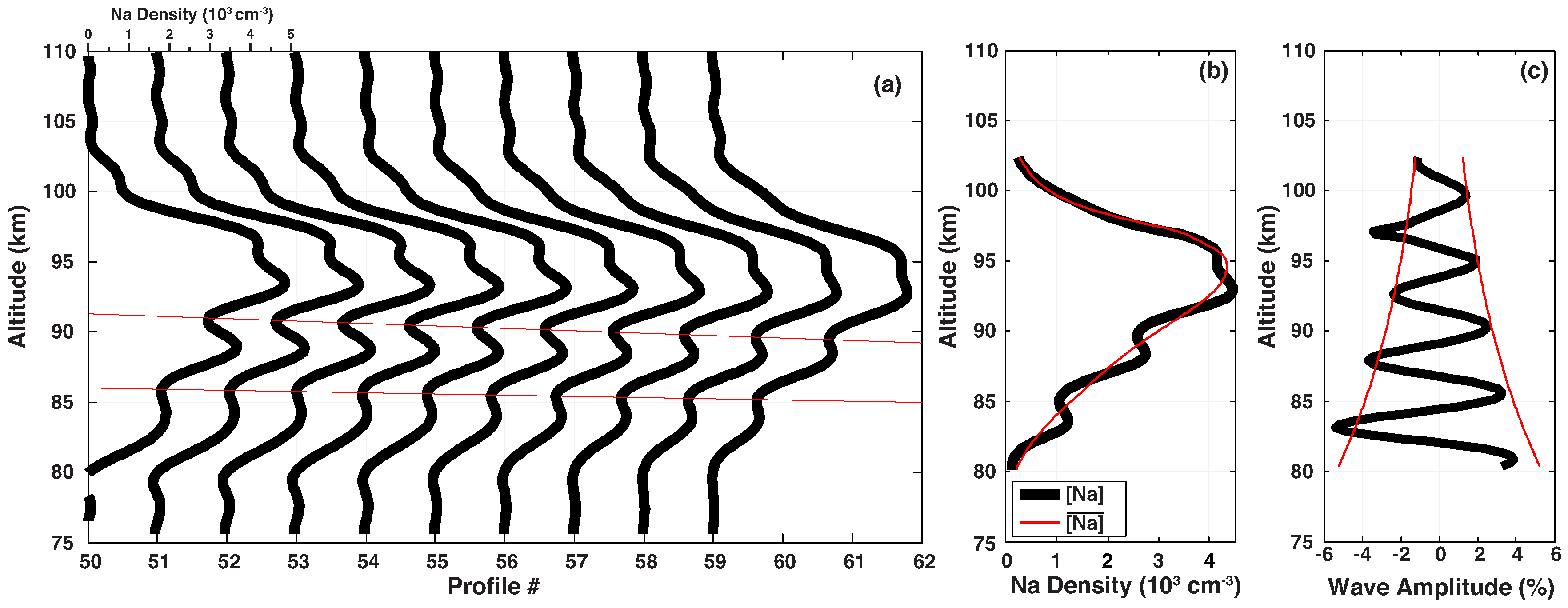
Figure 1 shows how the monochromatic waves are identified in sodium lidar data.
Figure 1a shows a temporal series of sodium lidar vertical density profiles from 75–110 km, with temporal resolution of 3 min and spatial resolution of 250 m. The sodium density profiles are first spatially and temporally low-pass filtered with cutoffs of about 1.5 km and 20 min, respectively. Coherent downward phase progression can be seen in
Figure 1 by the descending straight red lines. Additionally,
Figure 1b shows a single [Na] profile superposed to an estimated unperturbed
profile, which correspond to the average of seven profiles around the analyzed time. The relative wave amplitude perturbing the Na layer is given in
Figure 1c, showing a decreasing wave amplitude as it propagates upward because the wave phase descends with time as shown by the red thin lines in
Figure 1a. For this specific case, the wave presents vertical wavelength
km, amplitude of 2.46% relative to the ambient density (at 90 km), and inverse growth rate
km. Wave periods, horizontal wavelengths, and phase velocities can also be estimated using the technique described by [
12].
In addition to the lidar, a multicolor nightglow imager operating at Cachoeira Paulista (23
S, 45
W), 114 km away from the lidar site, provided images of the mesospheric nightglow layers for three emissions during the years of 1999, 2000, 2004, and 2005. A description of this imaging system is given in [
13].
To obtain the wave parameters, we first preprocess the image dataset by performing usual corrections in every image (i.e., unwarping, star removal, coordinate transformation, detrending, and filtering). Reference [
14] present the preprocessing methodology used in this study. We focus in wave events occurring quasi-simultaneously in two or three nightglow layers.
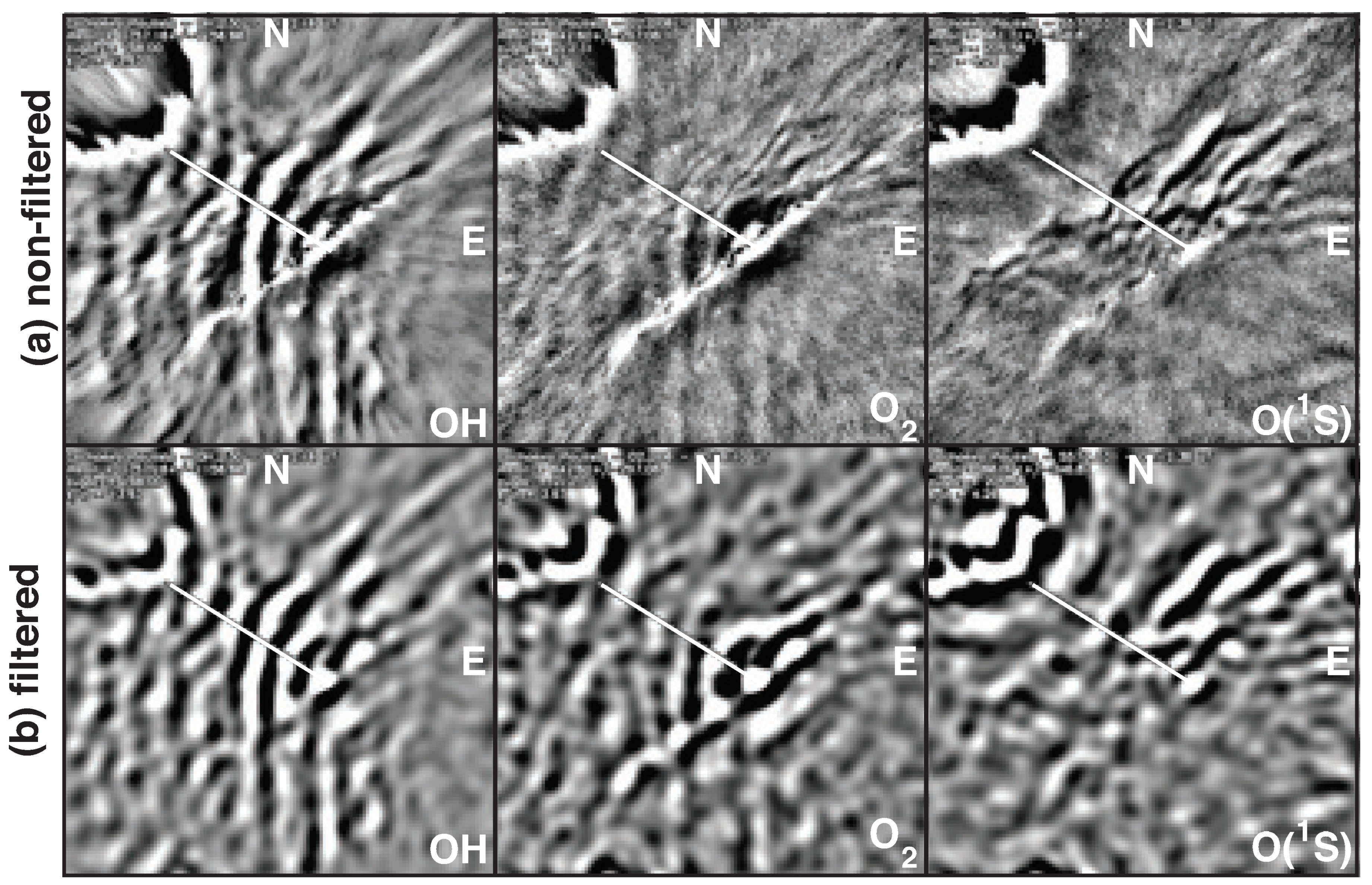
Figure 2a shows an example of a strong gravity wave simultaneously perturbing the central area of images of three nightglow emissions. We have spatially filtered the image set in order to increase the contrast of wave crests by using the Butterworth filter with cutoff wavenumbers at
km
and
km
. The result of the filtering operation is presented in
Figure 2b.
Images of the OH, O, and O() emissions showing simultaneously prominent gravity wave events are then submitted to 1D cross-spectral analysis to deduce the wave horizontal wavelength, phase difference at different layers, propagation direction, phase velocity, period, relative amplitude, and amplitude growth rate. Due to differences in integration times and filter wheel sequence cycle for every emission recorded by our imaging system, we have only been able to identify 52 wave events disturbing the three layers in four years of observations. Moreover, vertically propagating waves in image data have a short duration as their phase velocities are generally high, which challenges the observation of waves in the three emissions quasi-simultaneously.
The wave amplitude is obtained for a given nightglow layer by extracting relative intensity
along a straight line drawn perpendicularly to the wave fronts (see
Figure 2). These spatial series’ of pixel intensities of each layer can be seen in
Figure 3a. Each pair of series are then subjected to cross-spectral analysis from where amplitude and phase periodograms are obtained.
Figure 3b,c show the amplitude and phase periodograms of the spatial series showed in
Figure 3a. The uncertainty in the wave amplitude is less than 20% according to calculations of [
15]. As the layers peak at different altitudes and their separation (
) is a significant fraction of the wave’s vertical wavelength, a finite phase difference is expected to be measured in the phase cross-spectra. The uncertainty in
is 50% based on the work of [
15] as well.
The location of a spectral maximum in the amplitude periodogram indicates the horizontal wavelength of the dominant wave perturbing the airglow. By integrating the spectrum in the wavenumber range around the dominant spectral peak, we obtain an estimation of the relative wave amplitude. As the vertical distance
between the centroid of two given airglow layers is known, the amplitude growth rate is estimated by solving
. As the wave perturbs all three layers at the same time, we observe a finite phase difference for every spatial series pair (
Figure 3c). The layer centroid altitudes here have been assumed from simulations of the mesospheric nightglow layers [
8]. However, notice that the layer centroids and the relative layers’ separation changes slightly with season, location, etc. For example, see [
16].
By applying the procedure above to the images in
Figure 2, we have obtained the following parameters for the observed gravity wave event: horizontal wavelength of ∼40 km, period of ∼30 min, propagation direction of 160
, apparent phase speed of ∼20 m/s, and amplitude of 15%, 7%, and 5% in OH, O
, and O (
) layers, respectively, indicating a dissipative wave with
km
. We refer the reader to the work of [
17,
18] to find out more details of how wave parameters are derived from the cross-spectral analysis of airglow images.
We also estimate here the uncertainty of the amplitude growth rate for the wave in
Figure 2. Based on [
15], an expression for the uncertainty in the amplitude growth ratio is
The relative uncertainties in the amplitudes (, ) and layer separation () are 20% and 50%, respectively. Plugging in these values, we estimate a relative uncertainty for the amplitude growth rate. This represents an upper limit of once we have used worst-case scenario values for individual uncertainties of interest. This worst-case value for is taken as an estimation of the uncertainty for all the growth rates derived in this paper.
3. Results
There were 45 gravity wave events identified and analyzed from ten years of sodium lidar density profiles [
12] as well as 52 gravity wave events from four years of airglow images. Lidar and imager observations were not carried out simultaneously, but this fact does not affect our results since the two instruments sample distinct ranges of the gravity wave spectra, e.g., [
10].
Wave vertical scales accessed from lidar measurements are limited by the sodium layer thickness (∼15 km). On the other hand, the shortest accessible vertical wavelength is limited by the signal shot noise [
19]. For this reason, the waves identified from lidar data by [
12] presented vertical wavelengths in the 2.4–9.3 km range, with most of these waves (∼40%) within the 3–4 km interval. Observed wave periods ranged from 63 min to ∼20 h, with maximal occurrence (66%) in the 100–300 min range. The horizontal wavelengths fell within the
km range, but with predominant tendency of waves with
km. Wave amplitudes ranged from 0.77–8.4% of the ambient sodium density, with an average of 2.7%.
Gravity wave vertical wavelengths from imager measurements are larger than the airglow layer thicknesses [
8]. Typical layer thickness varies from 8 to 10 km. As the observed airglow intensity is given by vertical integration of the volume emission rate of the emission, short vertical scale waves (
km) are difficult to observe once they self-interfere within the layer. The wave intensity perturbation is strongly attenuated for ground-based observations in that case.
Imagers are able to observe short period waves ( h) and fast phase speeds ( m/s). The horizontal wavelength accessed with imager in this study was limited by the field of view of the instrument once we were focusing only on the phase of the wave in snapshots of the airglow emissions taken quasi-simultaneously. Notice, however, that larger horizontal wave scales can be seen via airglow imagery by sampling wave structures over the entire night. The lower limit is determined by the spatial resolution () of each pixel, which is 1 km/pixel in this study. Spectral analysis of the events studied here shows ranging from ∼14 to ∼78 km. The analysis of spatial series extracted from images reveals relative wave amplitudes () ranging from 0.6% to 15% for the OH, from 0.5% to 8.5% for O, and from 0.5% to 8.5% for O() emissions.
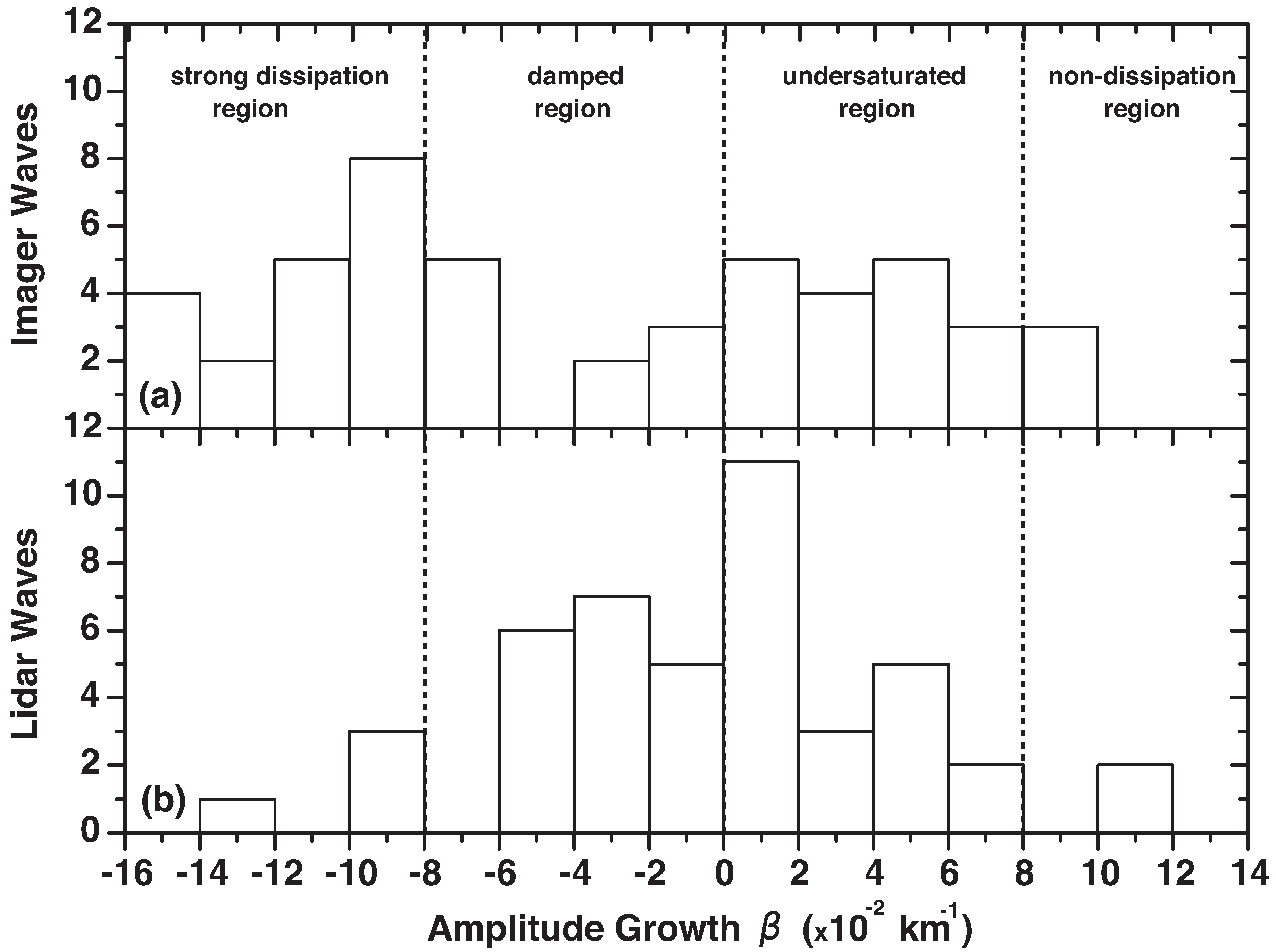
Figure 4 shows histograms for the amplitude growth rate (
) for waves observed in both imager and lidar data. Positive values of
indicate amplitude amplification with increasing altitude, while negative values refer to decay of the wave amplitude with increasing altitude. Values of
show that the amplitude does not change as the wave propagates upward (saturated wave), while events presenting
8
km
are nondissipating (freely propagating) waves as their amplitude e-folds every
12 km [
3]. Finally, waves presenting
km
decay in amplitude rapidly (strong dissipation), losing more than 64% of their original energy within
12 km distance.
Amplitude growth rates derived from lidar waves present 48.9% of negative values and 51.1% of positive values, showing a somewhat symmetric distribution of . For waves observed in imager data, there are 61.5% of negative and 38.5% of positive growth rate values, indicating a slight predominance of damped wave modes. Remarkably, only a small fraction of the observed wave events (4% imager; 9% lidar) are nondissipative (freely propagating waves), that is, few waves present growth close to the theoretical rate = km.
Wave events observed in Na lidar profiles show a maximal occurrence of waves in the range of [ km (undersaturated region) that represents 24% of total lidar waves. These events show amplification with increasing altitude but not as fast as the theoretical growth rate. In contrast, imager waves show the maximal growth rate occurrence in the [ km interval (strong dissipation region), which corresponds to 15.4% of the imager events.
About 36% of lidar waves are close to the saturation limit (
), in contrast with 16% of imager waves with similar behavior. In addition, ∼51.6% of the imager waves show strong attenuation (
km
) against only ∼9% of waves in the lidar dataset having similar growth rates. This contrast may be caused by the method of analysis used by [
12], which is biased towards waves that propagate normal to the wind flow, or are experiencing uniform Doppler shift along the Na layer.
4. Discussion
Our results show that imager waves are strongly dissipated within the MLT, decaying in amplitude in short distances (<12 km). Lidar waves tend to maintain a constant amplitude within the MLT region.
While nondissipating, propagating waves ( km) correspond to 9% and 4% of the events observed by lidar and imager, respectively, and about 90% of waves observed in both instruments show dissipative behavior (departures from the nondissipative wave growth rate ). The wave energy transferred to the media due to dissipative wave processes causes direct effects in the atmosphere, such as mean flow acceleration and local heating. In general, hydrodynamic instabilities and diffusion processes are responsible to limit the wave amplitude.
Imager waves present stronger dissipation than lidar waves in the
region of the distribution. The fact that imager waves present longer vertical wavelengths (
km) than lidar waves (
km) may shed light on this stronger dissipative behavior. Indeed, saturation theories, e.g., [
20,
21] invoke that various saturation processes constrain wave amplitudes at large vertical wavenumbers (smaller
). In the MLT, wave amplitudes may exceed saturation values where large group velocities impose wave amplitude growth that is faster than the time for instabilities to take over the dissipation process. Thus, the dissipation occurs via saturation of the wave amplitude, but neither via wave breaking nor turbulence.
The linear saturation theory (LST) predicts that the wave amplitude will reach the saturation limit when the horizontal perturbation velocity
equals the intrinsic horizontal phase velocity of the wave
. The amplitude is then limited by convective or shear instabilities [
20]. On the other hand, the diffusive filtering theory (DFT) states that waves will be severely damped by diffusion when the effective vertical diffusion velocity
of the particles experiencing the wave motion exceeds the vertical phase velocity of the wave
[
22]. Here,
D,
m, and
are the total effective atmospheric diffusivity, the vertical wavenumber, and the wave frequency, respectively.
In this sense, waves presenting
>
propagate without attenuation, while waves presenting
<
are removed from the spectra by diffusion. Our study as well as [
12] suggest that gravity waves observed in lidar measurements are in accordance with the DFT, while ruling out the predictions of the LST. However, some observed wave events in the lidar dataset presented peculiar behavior, suggesting that processes other than diffusivity have to be considered to explain the observed wave amplitude characteristics and growth rates.


