Mean Zonal Drift Velocities of Plasma Bubbles Estimated from Keograms of Nightglow All-Sky Images from the Brazilian Sector

Abstract

We present in this work a method for estimation of equatorial plasma bubble (EPB) mean zonal drift velocities using keograms generated from images of the OI 6300.0 nm nightglow emission collected from an equatorial station–Cariri (7.4° S, 36.5° W), and a mid-latitude station–Cachoeira Paulista (22.7° S, 45° W), both in the Brazilian sector. The mean zonal drift velocities were estimated for 239 events recorded from 2000 to 2003 in Cariri, and for 56 events recorded over Cachoeira Paulista from 1998 to 2000. It was found that EPB zonal drift velocities are smaller (≈60 ms⁻¹) for events occurring later in the night compared to those occurring earlier (≈150 ms⁻¹). The decreasing rate of the zonal drift velocity is ≈10 ms⁻¹/h. We have also found that, in general, bubble events appearing first in the west-most region of the keograms are faster than those appearing first in the east-most region. Larger zonal drift velocities occur from 19 to 23 LT in a longitude range from −37° to −33°, which shows that the keogram method can be used to describe vertical gradients in the thermospheric wind, assuming that the EPBs drift eastward with the zonal wind. The method of velocity estimation using keograms compares favorably against the mosaic method developed by Arruda, D.C.S, 2005, but the standard deviation of the residuals for the zonal drift velocities from the two methods is not small (≈15 ms⁻¹).

1. Introduction

Ionospheric equatorial plasma bubbles (EPB) are extensive spatial regions of accentuated reduction of ions along the magnetic field lines. In the EPB region, the electron density is rarefied due to instability processes appearing in the equatorial, low latitude area. The first observations of ionospheric EPBs in the Brazilian sector were reported by [1,2] using scanning photometers. Since then, this phenomenon has been extensively studied using radar [3,4,5,6] and optical techniques [7,8,9,10,11,12,13,14,15].

Studies revealed that ionospheric EPBs generally have strong correlations with the Spread F phenomena, with maximal occurrences in summer months, whereas in winter time only few bubble occurrences have been recorded [11]. It was also noticed that the EPBs were correlated with solar activity. For instance, Ref [16] reported an increase of 80% in their rate of occurrence during solar maxima. The dynamics of these EPBs include the less well-known seeding process after the sunset in equatorial latitudes following the upward movement and spreading of the plasma to low latitudes towards magnetic conjugate points along the geomagnetic field lines. This phenomenon has deep effects in the atmospheric region around 80 to 300 km of altitude, mainly in radio communication and GPS positioning throughout the equatorial region. The processes of seeding by gravity waves and growth of the Rayleigh–Taylor instability, responsible for the bubble’s vertical development, are not well understood yet [17,18].

Ionospheric EPBs usually present relatively large velocities towards the east and its spatial structure exhibits considerable time evolution [19]. These zonal drifts result from the vertical polarization electric fields, which are generated through complex interactions among the tidal winds, the geomagnetic field, and the ionospheric plasma in the F region. Consequently, EPBs are strongly aligned with the geomagnetic equator field lines, and their zonal drift velocities show large variability. In [15], they found that these velocities vary according to the month, decrease with the local time, and peak before local midnight. They also observed an increase of these velocities with the solar activity.

The aims of the present study were to determine the mean and instantaneous zonal drift velocities of EPBs events recorded in OI6300 nightglow image data and keograms. We have carried out a comparison of our keogram method for zonal drift velocities derivation with a another named mosaic method. In Section 2 we present the instrumentation, the database, and the methodology used to estimate zonal drift velocities of the EPB from keograms. Section 3 presents the results of the analysis and discusses our findings. Finally, Section 4 gives the main conclusions according to the discussion of the results.

2. Data and Methodology

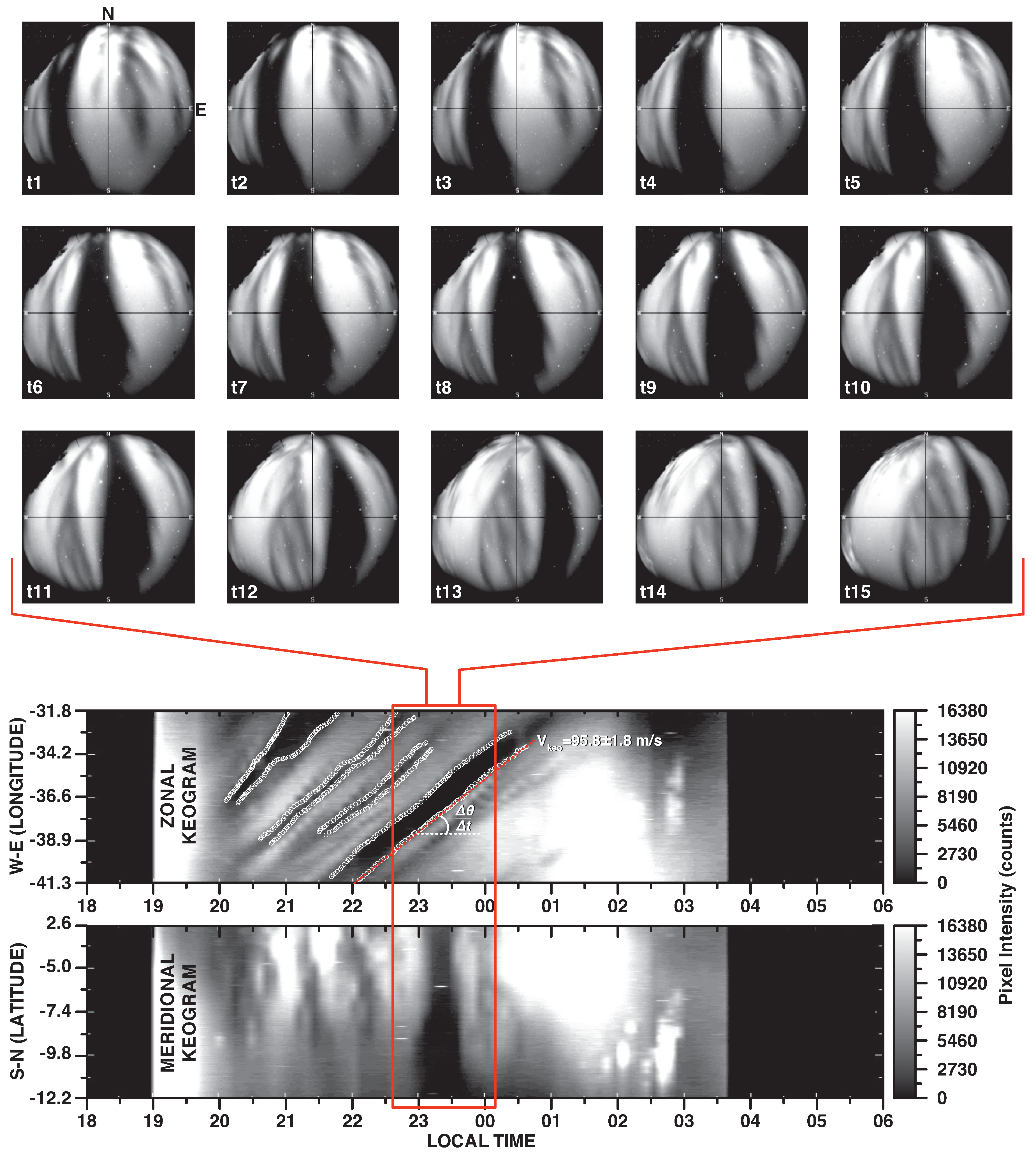
Original data used in this work are images of the OI6300 airglow emission obtained with all-sky CCD imagers operating at the low latitude station named Cachoeira Paulista (22.7° S, 45° W) (hereafter CP), and at the equatorial station named Cariri (7.4° S, 36.5° W) (hereafter CA), both in the Brazilian territory. A full discussion of how the redline is generated in the nighttime thermosphere can be found in [20] and references therein. A detailed description of the instruments used during the observation periods is given by [21]. In CA, 106 nights with the occurrence of EPBs were observed from 2000 to 2003, and 239 structures were identified using keograms built from the airglow images. For the CP station, 56 EPB events were observed from 1998 to 2000. Based on these records, it was possible to estimate the zonal drift velocities of these bubbles using west-east keogram images.

Keograms

Frequently, an EPB footprint appears in OI6300 airglow images and can be noticed as sporadic dark regions in the images. They are associated with ion density rarefaction in the ionosphere around ≈250–300 km of altitude for this specific wavelength emission. The keogram method used in this work summarizes the EPB behavior obtained from images along an entire night.

The word keogram comes from keoitt, an ancient Inuit word that means boreal aurora. In the beginning, the keograms were extensively used for studies of the auroral phenomenon in high latitudes. Afterwards, several areas began to use this technique including aeronomy done with optical probes.

In general, keograms are generated by extracting columns (south-north axis) and rows (west-east axe) from geographically mapped nightglow image data. The technique of keogram construction is illustrated in Figure 1. This method requires pre-processing of raw images prior any further analysis. The work of [22] describes in detail the pre-processing procedure that involves spatial calibration, star removal, geographic projection, re-gridding, and flat fielding of each image used in this study.

Here, the most important application of the keograms is related with clear signatures of EPBs in nightglow images. It is possible to calculate the mean zonal drift velocity of a given event (such as addressed in the next section) as well as its horizontal extension and duration. In addition, further information can be easily taken from the keogram images: the initial and final observation time, gaps in the data acquisition during the night due to either technical problems or unfavorable weather conditions (cloud cover or sources of light noise), etc.

Bubble signatures in the meridional keogram exhibit a wide dark region lying along of vertical axis. The bubble structure is inverted in this frame because the frontal portion of the bubble crosses earlier the center column of the original image. In zonal keograms, the signature appears as a tilted dark region relative to the temporal axis of the image. The mean zonal drift velocity of the bubble can be computed from the zonal keogram by estimating the tilt angle between the dark structure and the temporal axis.

The inclination angle and the mean velocity of a specific EPB event are related by the expression

$$v=\alpha \frac{\Delta \theta }{\Delta t},$$

where $\Delta \theta$ represents the longitude interval covered by the bubble structure in a given time interval $\Delta t$. The parameter $\alpha$ in this equation is a scale factor to convert the zonal drift velocity into proper physical units as follows. Raw airglow images are calibrated spatially by stellar coordinate mapping, and the spatial resolution $ds$ of each pixel is known, as is the pixel angular resolution $d\theta$. Also, the total latitude (longitude) angle covered by all-sky images at 250 km of altitude is known for our stations from geometrical modeling [22]. Thus, the parameter $\alpha$ can be defined to convert the zonal drift velocity from longitude per hour ($\Delta \theta /\Delta t$) to ms⁻¹.

We calculated the mean inclination angle through a linear fitting algorithm of manually specified pixels (white circles in Figure 1) along with the bubble structure, as observed in the keogram. An analysis script created to generate keograms allows to select pixels inside the tilted dark region that represents a given bubble event. The coordinates of the selected pixels (longitude, time) are stored and used as an input in the linear fitting procedure. The program calculates the best fit of the selected points, traces a straight line in the zonal keogram, and shows the slope of the linear fit, as presented in Figure 1, for the entire bubble structure representing the velocity of the whole event structure. The slope of the line is the averaged rate $\Delta \theta /\Delta t$. The mean zonal drift velocity of the event is obtained by multiplying the average slope by the scale parameter $\alpha$. In addition, we also use the same methodology with a 30 min running average of the selected points to obtain the instant zonal drift velocity of a bubble structure throughout the event’s duration.

3. Results

The first analysis was carried out by taking the mean zonal drift velocity of each bubble event in our dataset. As showed in the Figure 2a, the mean zonal drift velocity decreases with local time for both CA and CP stations. A decreasing rate of ≈10 ms⁻¹/h was found on the linear fit of the observed zonal drift velocities. The histogram of the distribution of velocities is in Figure 2b. The centers of distribution were in the 100 m/s bin for both sites, and they were both skewed to the right.

We also compared the keogram method presented here against the mosaic method developed by [9]. We used the exact same data set of EPB events for the comparison. We refer by $v_{mosaic}$ to the bubble zonal drift velocity calculated from the mosaic method, and by $v_{keo}$ to the zonal drift velocity estimated with the keogram method.

Figure 3a shows a correlative analysis for the velocities calculated by the two methods. The correlation coefficient between $v_{mosaic}$ and $v_{keo}$ is 0.85 (R² = 0.7). The uncertainty of linear fitting coefficients is also presented in the Figure 3 by the 95% bounds (gray dotted lines). The uncertainties are relatively small compared to the magnitude of each coefficient, showing that the methods are in good statistical agreement for the estimated zonal drift velocities.

The distribution of the residuals of $v_{mosaic}-v_{keo}$ is shown in Figure 3b. The mean value of the normal distribution for CA was 4.4 ms⁻¹ and the standard deviation is 16.4 ms⁻¹. For CP, the mean was 1.2 ms⁻¹ and the standard deviation is 14.2 ms⁻¹.

We obtained the instant zonal drift velocity of the bubble structure throughout the event duration by doing a 30 min running average of the selected pixels represented by the white circles in Figure 1 (bottom panel), allowing us to estimate the instant velocity every 30 min. Shown here is only the derivation carried out for CA station because it had a larger number of events detected over the years. The result is in Figure 4. Each color represents a distinct year of observation, while the numeral in parentheses is the number of events observed during the year. Observe that a continuous line of a given color shows how the drift of the EPB varies along its physical structure. Remarkably, some events showed positive drift velocity earlier, and then changed to being negative after some time, as in the example pointed out by the black arrow in Figure 4. This could be the result of a plasma drift reversal due to the background thermospheric zonal wind that is eastward during the night and westward during the day.

4. Discussion

We have shown that the mean zonal drift velocity decreases with local time. The decreasing rate of the drift velocity was ≈10 ms⁻¹/h for both CA and CP stations. This rate does not mean that bubbles decelerate as they move zonally, but it indicates that, if observed in later hours, bubbles are more likely to present slower drift velocities. Reference [15] found similar results at the low station of Cachoeira Paulista, Brazil. They calculated the decreasing rate of the mean zonal drifts of the bubbles ranging from 14.2 ms⁻¹/h to ≈8.5 ms⁻¹/h (Table 2, [15]), depending on the season and solar activity. The decreasing of the drift velocity of bubble events represents the influence of the neutral wind on the bubble dynamics. The polarization electric field that drives the F region nocturnal zonal drift is very intense after sunset and decreases with time because of the reduced neutral wind velocity, causing the ionospheric plasma to move by the $E\times B$ drift due to vertical electric fields generated by the zonal wind.

The comparison of the keogram method against the mosaic method developed by [9] shows somewhat large standard deviations for the normal distribution of $v_{mosaic}-v_{keo}$ in Figure 3b. This points out to a slight disagreement between the two methods. For instance, while ≈68% of the events present relative differences of less than ≈15 ms⁻¹, more than ≈30% of them have residuals larger than 15 ms⁻¹ for the estimated zonal drift velocity. Considering that the overall mean of observed zonal drift velocities is ≈100 ms⁻¹, the relative error would be larger than 15%. That points out that one third of the time the results from these two methods will differ by >15 ms⁻¹.

From the instant zonal drift velocity in Figure 4, we can show how the bubble drift varies with local time and longitude (Figure 5). This is possible because the keogram method allows for the mapping of the bubble velocity with longitude, as we record the time, position (longitude), and velocity along each portion of the bubble structure. For example, the event starting at 20 LT in Figure 2 shows that the tilt of the structure changes after 21 LT, as shown by the individual tiny white circles. Each circle contains information of the time and position of the structure that allows one to calculate the instant velocity of the bubble in the vicinity of that specific portion of the bubble structure.

To build the top panel of Figure 5, we used all the points (tiny white circles’ information) along all the observed bubble structures collected in CA. Based on that, we can see in the bottom panel of Figure 5 that larger zonal drift velocities appear in the west-most side of zonal keograms (−37° to −33° longitude). Also, in this latitude range between 21 and 23 LT, the zonal drift velocities are larger. This may be associated with the neutral wind behavior and a locally disturbed ionospheric dynamo. Notice that the bubble structure is an equatorial feature mapped to mid latitudes via the geomagnetic field lines. The taller the bubble structure is at the magnetic equator, the more south its structure will be mapped down in latitude and seen in images of the 630.0 nm airglow. Thus, the longitudinal gradient in the bubble drift velocity presented here evidences a vertical gradient in the thermospheric wind that controls plasma drifts in the nighttime F region ionosphere, with faster winds in the base of the bubble than near the top of it.

5. Summary and Conclusions

We presented in this work a new method to analyze ionosphere EPBs events and calculated their mean zonal drift velocities using keogram images. The data set comprises images of OI6300 nightglow emission obtained in Cariri (7.4° S, 36.5° W), an equatorial site, and Cachoeira Paulista (22.7° S, 45° W), a mid latitude site. Both stations are located over the Brazilian sector. Images from CA were taken from 2000 to 2003, while those in CP were from 1998 to 2000. The main findings of this work are:

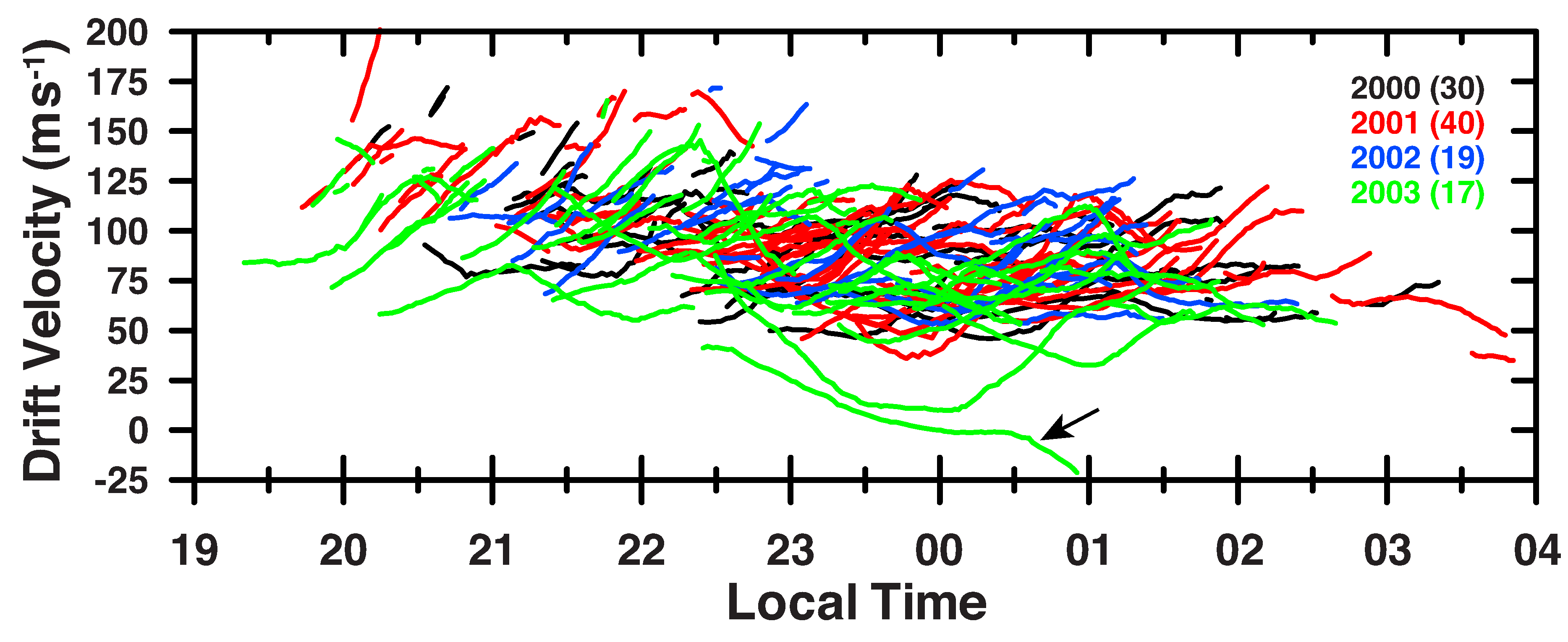
• In general, mean zonal drift velocities of EPBs decrease throughout the night. Larger velocity events travel at ≈150 ms⁻¹ (usually occurring during earlier hours of an observation period), while slower events move at ≈60 ms⁻¹ (occurring late in an observation period). The decreasing rate is ≈10 ms⁻¹/h.
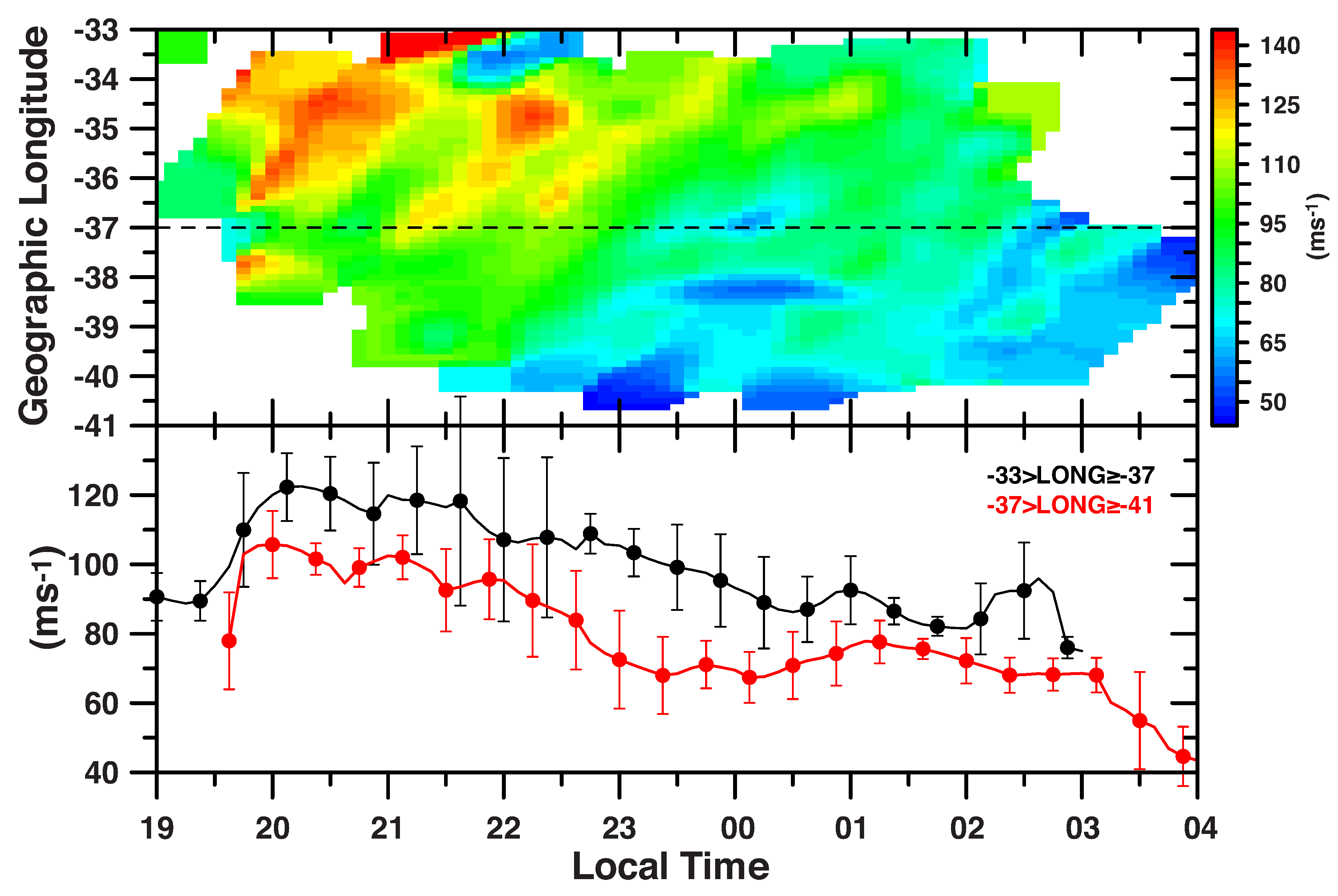
• Typically, faster EPBs occur from 20 LT to 23 LT in the west-most region of the zonal keograms in a longitude range of −37° to −33°. The longitudinal gradient in the bubble drift velocity indicates a vertical gradient in the thermospheric wind that controls plasma drifts in the nighttime F region ionosphere. The keogram method can be used to describe these vertical gradients in the thermospheric wind, assuming that the EPBs drift eastward with the zonal wind.
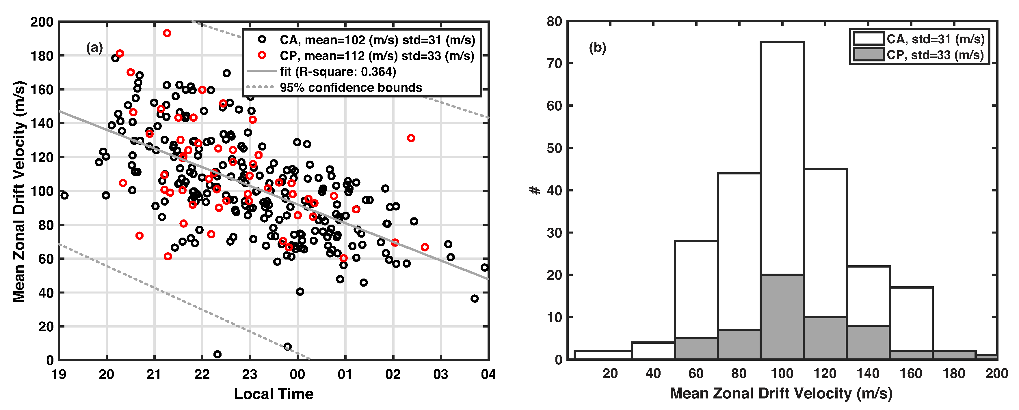
• Our keogram technique compares favorably with the mosaic method [9]. A Gaussian curve fits the velocity differences distribution of $v_{mosaic}-v_{keo}$ well. The standard deviation of the residuals distribution is large (≈15 ms⁻¹). Moreover, >30% of the residuals of $v_{mosaic}-v_{keo}$ have values larger than 15 ms⁻¹, which points out to possible refining of the methods.

References

1. Sobral, J.H.A.; Abdu, M.A.; Batista, I.S. Airglow studies on the ionosphere dynamics over low latitude in Brazil. Ann. Geophys. 1980, 36, 199–204. [Google Scholar]
2. Sobral, J.H.A.; Abdu, M.A.; Zamlutti, C.J.; Batista, I.S. Association between plasma bubble irregularities and airglow disturbances over Brazilian low latitudes. Geophys. Res. Lett. 1980, 7, 980–982. [Google Scholar] [CrossRef] [Green Version]
3. Abdu, M.A.; Muralikrishna, P.; Batista, I.S.; Sobral, J.H.A. Rocket observation of equatorial plasma bubbles over Natal, Brazil, using a high-frequency capacitance probe. J. Geophys. Res. Space Phys. 1991, 96, 7689–7695. [Google Scholar] [CrossRef]
4. Abdu, M. Outstanding problems in the equatorial ionosphere–thermosphere electrodynamics relevant to spread F. J. Atmos. Sol.-Terr. Phys. 2001, 63, 869–884. [Google Scholar] [CrossRef]
5. Dos Santos Prol, F.; Hernández-Pajares, M.; Tadeu de Assis Honorato Muella, M.; De Oliveira Camargo, P. Tomographic Imaging of Ionospheric Plasma Bubbles Based on GNSS and Radio Occultation Measurements. Remote Sens. 2018, 10, 1529. [Google Scholar] [CrossRef] [Green Version]
6. Silva, R.P.; Souza, J.R.; Sobral, J.H.A.; Denardini, C.M.; Borba, G.L.; Santos, M.A.F. Ionospheric Plasma Bubble Zonal Drift Derived From Total Electron Content Measurements. Radio Sci. 2019, 54, 580–589. [Google Scholar] [CrossRef] [Green Version]
7. Abalde, J.R.; Fagundes, P.R.; Bittencourt, J.A.; Sahai, Y. Observations of equatorial F region plasma bubbles using simultaneous OI 777.4 nm and OI 630.0 nm imaging: New results. J. Geophys. Res. Space Phys. 2001, 106, 30331–30336. [Google Scholar] [CrossRef] [Green Version]
8. Abalde, J.R.; Fagundes, P.R.; Sahai, Y.; Pillat, V.G.; Pimenta, A.A.; Bittencourt, J.A. Height-resolved ionospheric drifts at low latitudes from simultaneous OI 777.4 nm and OI 630.0 nm imaging observations. J. Geophys. Res. Space Phys. 2004, 109. [Google Scholar] [CrossRef] [Green Version]
9. Arruda, D.C.S. Study of the Nocturnal Ionosphere F-Layer Zonal Drifts over the Brazilian Region. Ph.D. Thesis, Instituto Nacional de Pesquisas Espaciais (INPE), São José dos Campos, Brazil, 2005. [Google Scholar]
10. Arruda, D.C.; Sobral, J.; Abdu, M.; Castilho, V.M.; Takahashi, H.; Medeiros, A.; Buriti, R. Theoretical and experimental zonal drift velocities of the ionospheric plasma bubbles over the Brazilian region. Adv. Space Res. 2006, 38, 2610–2614. [Google Scholar] [CrossRef]
11. Sobral, J.; Abdu, M.; Sahai, Y. Equatorial plasma bubble eastward velocity characteristics from scanning airglow photometer measurements over Cachoeira Paulista. J. Atmos. Terr. Phys. 1985, 47, 895–900. [Google Scholar] [CrossRef]
12. Sobral, J.H.A.; Abdu, M.A. Latitudinal gradient in the plasma bubble zonal velocities as observed by scanning 630-nm airglow measurements. J. Geophys. Res. Space Phys. 1990, 95, 8253–8257. [Google Scholar] [CrossRef] [Green Version]
13. Pimenta, A.; Bittencourt, J.; Fagundes, P.; Sahai, Y.; Buriti, R.; Takahashi, H.; Taylor, M. Ionospheric plasma bubble zonal drifts over the tropical region: A study using OI 630nm emission all-sky images. J. Atmos. Sol.-Terr. Phys. 2003, 65, 1117–1126. [Google Scholar] [CrossRef]
14. Takahashi, H.; Taylor, M.J.; Pautet, P.D.; Medeiros, A.F.; Gobbi, D.; Wrasse, C.M.; Fechine, J.; Abdu, M.A.; Batista, I.S.; Paula, E.; et al. Simultaneous observation of ionospheric plasma bubbles and mesospheric gravity waves during the SpreadFEx Campaign. Ann. Geophys. 2009, 27, 1477–1487. [Google Scholar] [CrossRef] [Green Version]
15. Terra, P.M.; Sobral, J.H.A.; Abdu, M.A.; Souza, J.R.; Takahashi, H. Plasma bubble zonal velocity variations with solar activity in the Brazilian region. Ann. Geophys. 2004, 22, 3123–3128. [Google Scholar] [CrossRef] [Green Version]
16. Sobral, J.; Abdu, M.; Takahashi, H.; Taylor, M.; de Paula, E.; Zamlutti, C.; de Aquino, M.; Borba, G. Ionospheric plasma bubble climatology over Brazil based on 22 years (1977–1998) of 630nm airglow observations. J. Atmos. Sol.-Terr. Phys. 2002, 64, 1517–1524. [Google Scholar] [CrossRef]
17. Taylor, M.J.; Eccles, J.V.; LaBelle, J.; Sobral, J.H.A. High resolution OI (630 nm) image measurements of F-region depletion drifts during the Guará Campaign. Geophys. Res. Lett. 1997, 24, 1699–1702. [Google Scholar] [CrossRef] [Green Version]
18. Takahashi, H.; Wrasse, C.M.; Figueiredo, C.A.O.B.; Barros, D.; Abdu, M.A.; Otsuka, Y.; Shiokawa, K. Equatorial plasma bubble seeding by MSTIDs in the ionosphere. Prog. Earth Planet. Sci. 2018, 5, 32. [Google Scholar] [CrossRef] [Green Version]
19. Schunk, R.; Nagy, A. Ionospheres: Physics, Plasma Physics, and Chemistry, 2nd ed.; Cambridge Atmospheric and Space Science Series; Cambridge University Press: Cambridge, UK, 2009. [Google Scholar] [CrossRef]
20. Vargas, F. Traveling Ionosphere Disturbance Signatures on Ground-Based Observations of the O(1D) Nightglow Inferred From 1-D Modeling. J. Geophys. Res. Space Phys. 2019, 124, 9348–9363. [Google Scholar] [CrossRef]
21. Medeiros, A.; Buriti, R.; Machado, E.; Takahashi, H.; Batista, P.; Gobbi, D.; Taylor, M. Comparison of gravity wave activity observed by airglow imaging at two different latitudes in Brazil. J. Atmos. Sol.-Terr. Phys. 2004, 66, 647–654. [Google Scholar] [CrossRef]
22. Garcia, F.J.; Taylor, M.J.; Kelley, M.C. Two-dimensional spectral analysis of mesospheric airglow image data. Appl. Opt. 1997, 36, 7374–7385. [Google Scholar] [CrossRef] [PubMed] [Green Version]
Figure 1. Illustration of how to build and derive the zonal drift velocity of an equatorial plasma bubble (EPB) from keogram images.
Atmosphere 11 00069 g001
Figure 2. (a) Mean zonal drift velocities of EPBs in Cariri (black) and Cachoeira Paulista (red) as functions of the local time. A linear fit (gray line) depicts that smaller velocities occur in later hours of the observation period. (b) Histogram of mean zonal drift velocity distributions for Cariri (white blocks) and Cachoeira (gray blocks).
Atmosphere 11 00069 g002
Figure 3. (a) Correlative analysis for zonal drift velocities obtained via the mosaic method against the keogram method. Back circles represent Cariri events, while red circles represent Cachoeira Paulista events. (b) Histogram of the difference between velocities computed via the mosaic method against the keogram method for Cariri (white blocks) and Cachoeira Paulista (gray blocks).
Atmosphere 11 00069 g003
Figure 4. Instant zonal drift velocities for EPBs in Cariri from 2000 to 2003 as a function of local time.
Atmosphere 11 00069 g004
Figure 5. (Top) Zonal drift velocity versus local time and geographic longitude for the Cariri observatory. (Bottom) Drift velocity versus time along distinct longitude ranges.
Atmosphere 11 00069 g005